How High Can The U-CAS Fly?

Abstract

The U-CAS is a spinning magnetized top that is levitated in a static magnetic field. The field is produced by a permanent magnet base, positioned below the hovering top. In this paper we derive upper and lower bounds for $h_{m}$–the maximum hovering height of this top. We show that the bounds are of the form $al_{0}$ where $a$ is a dimensionless number ranging from about $1$ to $12$, depending on the constraints on the shape of the base and on stability considerations, and $l_{0}$ is a characteristic length, given by

$$l_{0}\equiv\dfrac{\mu_{0}}{4\pi}\dfrac{\mu M_{0}}{mg}\text{.}$$

Here, $\mu_{0}$ is the permeability of the vacuum, $\mu$ is the magnetic moment of the top, $M_{0}$ is the maximum magnetization of the base, $m$ is the mass of the top, and $g$ is the free-fall acceleration. For modern permanent magnets we find that $l_{0}\sim 1$[meter], thus limiting $h$ to about few meters.

Index Terms– U-CAS, Levitron, magnetic trap, magnetic levitation, hovering magnetic top.

I Introduction

I-A What is the U-CAS?

The U-CAS is an ingenious device that hovers in mid-air while spinning. It is marketed as a kit in Japan under the trade name U-CAS [1], and in the U.S.A. and Europe under the trade name Levitron${}^{\text{TM}}$ [2, 3, 4]. The whole kit consists of three main parts: A magnetized top which weighs about $18$ gr, a thin (lifting) plastic plate and a magnetized square base plate (base). To operate the top one should set it spinning on the plastic plate that covers the base. The plastic plate is then raised slowly with the top until a point is reached in which the top leaves the plate and spins in mid-air above the base for about 2 min. The hovering height of the top is approximately $3$ cm above the surface of the base whose dimensions are about 10 cm $\times$ 10 cm $\times$ 2 cm. The kit comes with extra brass and plastic fine tuning weights, as the apparatus is very sensitive to the weight of the top. It also comes with two wedges to balance the base horizontally.

I-B The adiabatic approximation.

The physical principle underlying the operation of the U-CAS relies on the so-called ‘adiabatic approximation’ [5, 6, 7]: As the top is launched, its magnetic moment points antiparallel to the magnetization of the base in order to supply the repulsive magnetic force which will act against the gravitational pull. As the top hovers, it experiences lateral oscillations which are slow ( $\Omega_{\text{lateral}}\simeq 1$ Hz) compared to its precession ($\Omega_{\text{precession}}\sim 5$ Hz). The latter itself, is small compared to the top’s spin ($\Omega_{\text{spin}}\sim 25$ Hz). Since $\Omega_{\text{spin}}\gg\Omega_{\text{precession}}$ the top is considered ‘fast’ and acts like a classical spin. Furthermore, as $\Omega_{\text{precession}}\gg\Omega_{\text{lateral}}$ this spin may be considered as experiencing a slowly rotating magnetic field. Under these circumstances the spin precesses around the local direction of the magnetic field $\mathbf{B}$ (adiabatic approximation) and, on the average, its magnetic moment $\mathbf{\mu}$ points antiparallel to the local magnetic field lines. In view of this discussion, the magnetic interaction energy which is normally given by $-\mathbf{\mu}\cdot\mathbf{B}$ is now given approximately by $\mu\left|\mathbf{B}\right|$. Thus, the overall effective energy ‘seen’ by the top is

$$E_{\text{eff}}\left(\mathbf{r}\right)\simeq mgz+\mu\left|\mathbf{B}\left(\mathbf{r}\right)\right|,$$ (1)

where $m$ is the mass of the top, $g$ is the free-fall acceleration and $z$ is the height of the top above the base. By virtue of the adiabatic approximation, two of the three rotational degrees of freedom are coupled to the transverse translational degrees of freedom, and as a result the rotation of the axis of the top is already incorporated in Eq.(1). Thus, under the adiabatic approximation, the top may be considered as a point-like particle whose only degrees of freedom are translational. The important point of this discussion is the following: The energy expression written above possesses a minimum for certain values of $\mu/mg$. Thus, when the mass is properly tuned, the apparatus acts as a trap, and stable hovering becomes possible. A detailed description of this device, extending beyond the adiabatic approximation, may be found elsewhere  [6, 8, 9]. For the purpose of this paper, the adiabatic approximation will suffice.

I-C The limitations on the hovering height.

In this paper we focus on the question:

How high can the hovering height of the U-CAS be?

First, we define what do we mean by ‘height’: We assume that the top hovers above some horizontal plane. The height of the top is measured with respect to that plane. The ‘rules of the game’ are, that we can put permanent magnet below the plane, but never above this plane. Whatever is below this plane, will be called ‘the base’. The method we use to answer the question above will be by getting upper and lower bounds for this height, denoted by $h_{m}$. We begin by pointing out the factors that limit the hovering height of the U-CAS.

First, we set aside the question of stability and assume that the top is guided by a vertical axis, allowing it to move only axially (up and down). In this case, the easiest way to increase $h$–the hovering height, is by using a more powerful magnet for the base. This technique however, cannot be applied indefinitely since there is no way to increase the magnetization of a given substance without limit. We are therefore forced to limit the strength of $\mathbf{M(r)}$–the magnetization density of the base, to some maximum value, say $M_{0}$, and design the shape and magnetization density of the base so as to maximize $h$. One more factor that limits the levitation height is the amount of magnetic substance, or volume, in our disposal. Clearly, the more material we use, the larger is the levitation height that can be achieved. But still, even if the volume is infinite the levitation height is bounded, since $\left|\mathbf{M(r)}\right|$ is bounded.

When stability is taken into account, things get more complicated. Stability sets another limitation on the design of the base, in addition to the limitations that were discussed above: A brief look at Eq.(1) tells us that for the top to hover stably over the plate, the effective energy $E_{\text{eff}}$ should possess a minimum. This means, in particular, that

$$\dfrac{\partial^{2}E_{\text{eff}}\left(\mathbf{r}\right)}{\partial\mathbf{r}^{2}}\sim\dfrac{\partial^{2}\left|\mathbf{B}\left(\mathbf{r}\right)\right|}{\partial x^{2}},\dfrac{\partial^{2}\left|\mathbf{B}\left(\mathbf{r}\right)\right|}{\partial y^{2}},\dfrac{\partial^{2}\left|\mathbf{B}\left(\mathbf{r}\right)\right|}{\partial z^{2}}>0\text{,}$$ (2)

where the derivatives are evaluated at the equilibrium position of the top. Since these are homogenous inequalities, it is clear that the region in space where a minimum may occur, does not depend on the strength of the magnetic field. As a consequence, the hovering height of the U-CAS is not determined by the strength of the magnetic field but on its geometry, or alternatively, by the shape of the base. As an example, it has been shown [10] that for a vertically magnetized base in the shape of a disk of radius $R$, the range of heights $h$ for which stable hovering is possible, is very narrow and is around $h\sim R/2$. This result agrees roughly with the parameters of the U-CAS, for which $R\sim 10$ cm and $h\sim 4$ cm, when $h$ is measured from the center-of-mass of the base. The strength of the field then comes into play by tuning it in order to achieve equilibrium for a given mass of the top. Equilibrium prevails when the total force on the top vanishes, i.e. when

$${\mathbf{F}{=-\nabla}}E_{\text{eff}}=-mg{\mathbf{\hat{z}}}-\mu{\mathbf{\nabla}}\left|{\mathbf{B(r)}}\right|=0\text{.}$$ (3)

Both in the guided case and in the stable case, we see that in order to increase the hovering height of the U-CAS, we should design a better base. We do expect however, that the hovering height cannot be increased indefinitely. In connection with the redesigning of the base, we have recently shown [11], both theoretically and experimentally, that the use of a vertically magnetized ring of radius $R$ as a base, increases the hovering height by more than three times to about $1.7R$!. This increase in height did not came without cost, as the tolerance on the mass of the top became more stringent, being $\Delta m/m\sim 0.6\%$ for the ring vs. $\Delta m/m\sim 1.2\%$ in the case of the disk [10].

I-D The structure of this paper.

All the calculations that we do are outlined in Sec.(II). We will now describe what we calculate and what is the motivation behind it.

We start in Sec.(II-A), by deriving a close form expression for the first and second derivatives of the magnetic field, in terms of the magnetization density of the base. The first derivative is the magnetic force on the top, which is used throughout the paper, while the second derivative is exploited when we discuss stability.

In Sec.(II-B) we consider the problem of maximizing the hovering height in the case where the volume of the base may be infinite, and may be arbitrarily magnetized under the constraint that $\left|\mathbf{M(r)}\right|=M_{0}$. We still do not require that the top be stable against lateral translations, and assume that it is guided along a vertical axis. We show that in this case

$$h_{\max}\simeq 12l_{0},$$

where $l_{0}$ is a characteristic height for the problems that are discussed in this paper. It is defined as

$$l_{0}\equiv\dfrac{\mu_{0}}{4\pi}\dfrac{\mu M_{0}}{mg},$$

where $\mu_{0}$ is the magnetic permeability of the vacuum, $\mu$ is the magnetic moment of the top, $m$ is the mass of the top, and $g$ is the free-fall acceleration.

In Sec.(II-C) we consider the same problem as before but for a base which is uniformly magnetized along the vertical direction, namely ${\mathbf{M(r)}}=M_{0}{\mathbf{\hat{z}}}$, where $\mathbf{\hat{z}}$ is a unit vector in the vertical direction. In this case we find that

$$h_{\max}\simeq 3.5l_{0}.$$

In order to arrive to better bounds on $h_{m}$, our next step is to limit the amount of material available for the base. Thus, in Sec.(II-D) we maximize the hovering height in the case where the base may be arbitrarily magnetized under the constraint that $\left|\mathbf{M(r)}\right|=M_{0}$, and that its volume $V_{0}$ is given. Here, the result is given in the form of a plot, showing the dependence $h_{\max}$ on $V_{0}$. In the limit $V_{0}\rightarrow\infty$, we recover the result of Sec.(II-B). Our derivation is also constructive in the sense that it shows how to construct the optimal base for a given $V_{0}$. In this paper however, we do not discuss this matter thoroughly due to space shortage.

For completeness, we study in Sec.(II-E) the same problem as in Sec.(II-D), but for a uniformly magnetized base. Here, again we find the dependence of $h_{\max}$ on $V_{0}$ and recover the result of Sec.(II-C).

Sec.(II-F) is the first part where stability is added into play: We begin by explaining how to test for stability of the top under the adiabatic approximation, and study the possible levitation heights of a uniformly magnetized base whose shape is cylindrical of volume $V_{0}$. As the stability condition is given in the form of inequality relations (see Eq.(2)), it is not suffice to determine uniquely  the levitation height. We therefore choose to study two particular stable points: an isotropic stable point and the highest possible stable point. The meaning of these points would become clear later. In this case we also give a plot, showing the dependence of $h_{\max}$ on $V_{0}$. This result should also be considered as a lower bound for $h_{m}$, since the cylindrical base is a special case of all the base configurations that are possible.

In section(II-G) we take one step further, and generalize the result of section(II-F) to the case of a base which may be arbitrarily magnetized, and look for the lowest possible stable point. In this case however, we assume that $V_{0}=\infty$, to ease the solution of the problem. We also show that in this case, where $h_{\max}\simeq 8.4l_{0}$ and $V_{0}=\infty$, the lowest possible stable point and the highest one coincide, so this result represent not a bound for $h_{m}$, but is actually $h_{m}$ itself, for the case $V_{0}=\infty$.

In Sec.(III) we discuss interesting aspects of our results. In particular we estimate the value of $l_{0}$ for modern permanent magnet materials and calculate the values of the bounds for $h_{m}$. We comment on the implications of our results and discuss other related questions.

II Mathematical Formulation

II-A The upward magnetic force and its derivative.

A simplified model of the U-CAS is shown in Fig.(1). It consists of a point-like particle of mass $m$ and magnetic moment $\mu$ (pointing downward), hovering at a height $h$ above the $z=0$ plane. For the moment, we consider the top as if it was guided along the $z$-axis so that only its vertical motion is allowed. Other degrees of freedom are considered ‘frozen’. The region $z<0$ may be partially or wholly filled with a magnetized substance (“base”), whose magnetization density is denoted by $\mathbf{M(r)}$, producing a magnetic field throughout space which we denote by $\mathbf{B(r)}$. In what follows, we assume that the base (and hence the magnetic field) has a cylindrical symmetry around the $z$-axis. Thus, along this axis the magnetic field possesses only a $z$-component. We further assume that this component is positive, namely that the magnetic field along the $z$-axis is pointing upward.

Using Eqs.(1),(3) we find that, when the top is in equilibrium, the total vertical component of the force on the top vanishes,

$${\mathbf{F}}_{z}=-mg{\mathbf{\hat{z}}}-\mu\dfrac{\partial\left|{\mathbf{B}}\right|}{\partial z}{\mathbf{\hat{z}}}=0,$$

where the term $-mg{\mathbf{\hat{z}}}$ is the gravitational force pulling the top towards the base, and the term $-\mu{\mathbf{\hat{z}}}\partial\left|{\mathbf{B}}\right|/\partial z$ is the magnetic force which pushes the top upward. Note that $\partial\left|{\mathbf{B}}\right|/\partial z$ should be negative.

Since the top is allowed to move only along the $z$-axis, we may write $\left|\mathbf{B}\right|=B_{z}$ (in what follows we deserve the notation $B_{z}$ to denote the $z$-component of the magnetic field along the $z$-axis, namely $B_{z}\equiv{\mathbf{\hat{z}\cdot B}}\left(x=0,y=0,z\right)$). Now, the magnetic force on the top simplifies to

$${\mathbf{F}}_{m}=-\mu\frac{\partial B_{z}}{\partial z}{\mathbf{\hat{z}},}$$

and hence, when the top is in equilibrium at $z=h$,

$$-\mu\left.\frac{\partial B_{z}}{\partial z}\right|_{z=h}=mg.$$ (4)

Reciprocity allows us to express $\partial B_{z}/\partial z$ in terms of $\mathbf{M(r)}$ as

$$\frac{\partial B_{z}}{\partial z}=\int{\mathbf{M(r}}^{\prime})\cdot\frac{\partial{\mathbf{B}}_{d}({\mathbf{r}}^{\prime};z)}{\partial z}d^{3}r^{\prime}.$$ (5)

Here, ${\mathbf{B}}_{d}({\mathbf{r}}^{\prime};z)$ is the field at the point $\mathbf{r}^{\prime}$ produced by a unit magnitude dipole pointing upward, located at a height $z$ along the $z$-axis. Taking $r$ and $\theta$ as depicted in Fig.(1), we can write ${\mathbf{B}}_{d}$ as

$${\mathbf{B}}_{d}=\frac{\mu_{0}}{4\pi}\frac{(3\cos\theta{\mathbf{\hat{r}-\hat{z}}})}{r^{3}},$$ (6)

where $\mathbf{\hat{r}}$ is a polar unit vector, also defined in Fig.(1), and $\mu_{0}$ is the magnetic permeability of the vacuum. It is worth to note that $\partial{\mathbf{B}}_{d}/\partial z$ is nothing but the field produced at $\mathbf{r}^{\prime}$ by a quadruple located at a height $z$ along the $z$-axis. This quadruple is made out of a pair of identical dipoles: One is located at $z$ and pointing downward and the other is at an infinitesimally higher position $z+dz$ and pointing upward, with their magnetic moment being $1/dz$.

When Eq.(6) is substituted into Eq.(5) we find that, at $z=h$, the field derivative is given by

$$\left.\frac{\partial B_{z}}{\partial z}\right|_{z=h}=\frac{\mu_{0}}{4\pi}{\displaystyle\int\limits_{\pi/2}^{\pi}}\sin\theta d\theta{\displaystyle\int\limits_{-h/\cos(\theta)}^{\infty}}2\pi r^{2}dr\frac{1}{r^{4}}{\mathbf{M}}(r,\theta)\cdot\overline{{\mathbf{n}}}(\theta),$$ (7)

where

$$\overline{\mathbf{n}}(\theta)\equiv 6\sin\theta\cos\theta{\mathbf{\hat{\theta}}}+3(3\cos^{2}\theta-1){\mathbf{\hat{r}},}$$ (8)

and where ${\mathbf{\hat{\theta}}}$ is a polar unit vector orthogonal to $\mathbf{\hat{r}}$, as is shown in Fig.(1).

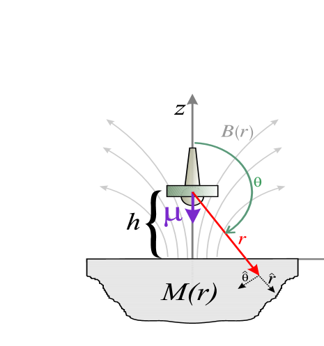
Figure 1: The U-CAS is modeled as a point-like particle of mass $m$ and magnetic moment $\mu$ pointing downward, hovering at a height $h$ above a non-uniformly magnetized base with magnetization density $\mathbf{M(r)}$ producing a field $\mathbf{B(r)}$.

We would also need the second derivative of the field, when we discuss stability. It is given by

$$\left.\frac{\partial^{2}B_{z}}{\partial z^{2}}\right|_{z=h}=\frac{\mu_{0}}{4\pi}{\displaystyle\int\limits_{\pi/2}^{\pi}}\sin\theta d\theta{\displaystyle\int\limits_{-h/\cos(\theta)}^{\infty}}2\pi r^{2}dr\frac{1}{r^{5}}{\mathbf{M}}(r,\theta)\cdot\overline{\mathbf{s}}(\theta),$$ (9)

where

$$\overline{\mathbf{s}}(\theta)\equiv 9\sin\theta\left(5\cos^{2}\theta-1\right){\mathbf{\hat{\theta}}}+12\cos\theta(5\cos^{2}\theta-3)\mathbf{\hat{r}.}$$ (10)

Note that in both Eqs.(7) and (9), ${\mathbf{M}}(r,\theta)$ is defined with respect to a polar coordinate system whose origin is at $z=h$ and not at $z=0$. Also note, that in going from Eq.(7) to Eq.(9), one should take into account the dependence of the unit vectors ${\mathbf{\hat{\theta}}}$ and $\mathbf{\hat{r}}$ on $z$.

II-B Arbitrarily magnetized, infinite base.

We consider an infinitesimal volume element at some point $(r,\theta)$ within the base. It is essentially a magnetic dipole whose magnitude is $M_{0}$, and whose direction we will now find by the requirement that the magnetic force on the top is maximized. We have already shown that the force on the top, contributed by one elemental dipole, is proportional to the magnetic field ${\mathbf{B}}_{d}$ that would be produced at $(r,\theta)$ by a quadruple located at $z=h$. To make this force maximal we assign to each point $(r,\theta)$ in $z<0$, a magnetization density $\mathbf{M(r)}$ whose magnitude is $M_{0}$ and whose direction is antiparallel to the field line of ${\mathbf{B}}_{d}$ at that point. The magnetization density so defined will maximize the force on the top, and is therefore the requested answer. Mathematically, this procedure amounts to replacing $\mathbf{M(r)}$ in Eq.(7) by ${\mathbf{M(r)}}=-M_{0}{\mathbf{\hat{n}}}(\theta)$, where ${\mathbf{\hat{n}}}(\theta)$ is a unit vector parallel to $\overline{\mathbf{n}}(\theta)$, the latter being defined in Eq.(8). The result is

$$\left.\dfrac{\partial B_{z}}{\partial z}\right|_{z=h} =-\dfrac{\mu_{0}}{4\pi}6\pi M_{0}{\displaystyle\int\limits_{\pi/2}^{\pi}}d\theta\sin\theta\sqrt{4\cos^{4}\theta+\sin^{4}\theta}$$

$$\times{\displaystyle\int\limits_{-h/\cos(\theta)}^{\infty}}\dfrac{1}{r^{2}}dr,$$

for which the $r$ integration is trivial and the $\theta$ integration may be brought to a simpler form by the transformation $x=\sin^{2}(\theta)$. This gives [12]

$$\left.\dfrac{\partial B_{z}}{\partial z}\right|_{z=h}=-\dfrac{\mu_{0}}{4\pi}\dfrac{3\pi M_{0}}{h}{\displaystyle\int\limits_{0}^{1}}\sqrt{4(1-x)^{2}+x^{2}}dx\cong-\dfrac{12M_{0}}{h}\dfrac{\mu_{0}}{4\pi},$$

which together with Eq.(4) shows that

$$h_{\max}\cong 12l_{0}\text{,}$$ (11)

where

$$l_{0}\equiv\dfrac{\mu_{0}}{4\pi}\dfrac{M_{0}\mu}{mg},$$

is the characteristic length in our problem which will reappear in the next sections. The value of $l_{0}$ may be interpreted as the distance between two colinear dipoles, one of them is of strength $\mu$ while the other is of strength $M_{0}l_{0}^{3}$, for which the mutual force between them is $mg$.

Eq.(11) shows that even though the magnetization direction is allowed to vary everywhere inside the base, the levitation height $h$ is bounded. Eq.(11) presents the maximum height that can be accomplished with a given substance provided that the top is not allowed to move laterally. Clearly, it also serve as an upper bound for $h_{m}$, as stability was not considered yet. Moreover, note that we have calculated the maximum magnetic force, which is proportional to $\partial B_{z}/\partial z$. The magnetic field $\left.B_{z}\right|_{z=h}$ on the other hand, becomes infinite at $z=h,$ as can be seen by the following simple argument: Since each elemental dipole within the plate contributes a field that goes as $1/r^{3}$ and since the volume of integration goes as $r^{2}$, the integrand goes as $1/r$, for which the integral diverges as $r\rightarrow\infty$. Later we show that the divergence of $\left.B_{z}\right|_{z=h}$ implies that the top cannot be stable when placed in such a point. In any case, it would be impossible to spin the top.

II-C Uniformly magnetized, infinite base.

Uniformly magnetized plates are clearly easier to construct. In this section we find out what upper bound does this restriction sets on the highest levitation point. In another sense, the result of this section may also be considered as a lower bound on the height of levitation (for a top which is guided!), provided one considers all possible base configurations.

We again consider an infinitesimal volume element within the base. It is now oriented along the $z$-direction and interacting with the top’s magnetic dipole. If this element is exactly below the top (i.e. it is located somewhere on the negative $z$-axis), it exerts a repelling $z$-directed force on the top, pushing it away. If the element is not exactly below the top then the nature of this force (i.e. weather it is repulsive or attractive) is determined by the angle formed between the direction of the two dipoles (in this case both point in the $z$-direction), and the direction defined by the line joining these dipoles. We call this angle $\theta$, and measure it with respect to the positive $z$-direction, as is shown in Fig.1.

There exists a critical angle $\theta_{0}$ (see Fig.(2)), for which the $z$-directed force vanishes such that for $\pi/2<\theta<\theta_{0}$ the force becomes attractive. It is therefore useless to put any material within the region $\pi/2<\theta<\theta_{0}$ and $(2\pi-\theta_{0})<\theta<3\pi/2$ since this would reduce the magnetic force and decrease the levitation height.

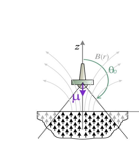
Figure 2: For a uniformly magnetized base, all the dipoles that lie within the angular sector $\theta_{0}<\theta<(2\pi-\theta_{0})$ (black dipoles), where $\theta_{0}\simeq 141^{0}$, repel the top. The dipoles that are outside this sector (grey dipoles) attract the top. Material should be put only in the repulsive sector.

To find $\theta_{0}$ we eliminate the $z$-component of Eq.(8), and find the value of $\theta$ for which it vanishes. We pick the value of $\theta$ that lies between $\pi/2$ and $\pi$. This gives

$$\theta_{0}=\pi-\arccos\sqrt{3/5}\cong 141^{o}.$$

We now evaluate the upward force exerted on the top, by summing the contributions of all the elements in the base located within $\theta_{0}<\theta<(2\pi-\theta_{0})$. The (uniform) magnetization density within this region is taken to be ${\mathbf{M(r)}}=M_{0}{\mathbf{\hat{z}}}$. Using Eq.(7), we find that

$$\left.\dfrac{\partial B_{z}}{\partial z}\right|_{z=h} =\frac{\mu_{0}}{4\pi}{\displaystyle\int\limits_{\theta_{0}}^{\pi}}\sin\theta d\theta{\displaystyle\int\limits_{-h/\cos(\theta)}^{\infty}}2\pi r^{2}dr\frac{1}{r^{4}}(M_{0}{\mathbf{\hat{z}}})$$

$$\cdot[6\sin\theta\cos\theta{\mathbf{\hat{\theta}}}+3(3\cos^{2}\theta-1)\mathbf{\hat{r}}]\text{.}$$

The integration over $r$ is again trivial, and we are left with an integration over $\theta$. The latter is brought to a simpler form by changing the $\theta$ variable into $x=\cos\theta$, hence

$$\left.\dfrac{\partial B_{z}}{\partial z}\right|_{z=h} =-\frac{\mu_{0}}{4\pi}\frac{6\pi M_{0}}{h}{\displaystyle\int\limits_{-1}^{-\sqrt{3/5}}}(5x^{4}-3x^{2})dx$$

$$=-\frac{\mu_{0}M_{0}}{h}\left(\dfrac{3}{5}\right)^{5/2}.$$

This result, together with the equilibrium condition Eq.(4), suggests that in this case the maximal levitation height possible is

$$h_{\max}=4\pi\left(\dfrac{3}{5}\right)^{5/2}\left[\dfrac{M_{0}\mu}{mg}\dfrac{\mu_{0}}{4\pi}\right]\equiv 4\pi\left(\dfrac{3}{5}\right)^{5/2}l_{0}\cong 3.5l_{0}\text{.}$$ (12)

Note, however, that in order to realize the levitation heights found in this section and in the previous one we would need an unlimited supply of magnetic material. In the following sections we find how good can we do when the volume of the base is constrained.

II-D Arbitrarily magnetized, finite base.

Under a given volume $V_{0}$, we find the optimum shape and magnetization of the base, that will maximize the levitation height. We use the Lagrange’s multipliers method to treat this variational problem [13].

First, we parametrize the shape of the plate: Let $r_{e}(\theta)$ be the upper integration radius, as is shown in Fig.(3). The lower integration radius is $-h/\cos\theta$. Utilizing the cylindrical symmetry of the problem, the volume may be written as

$$\begin{array}[c]{c}V=2\pi{\displaystyle\int\limits_{\theta_{1}}^{\pi}}\sin\theta d\theta{\displaystyle\int\limits_{-h/\cos\theta}^{r_{e}(\theta)}}r^{2}dr\\ =\dfrac{2\pi}{3}{\displaystyle\int\limits_{\theta_{1}}^{\pi}}d\theta\sin\theta\left(r_{e}^{3}(\theta)+\dfrac{h^{3}}{\cos^{3}\theta}\right),\end{array}$$ (13)

where the angle $\theta_{1}$ is determined by the condition that

$$r_{e}(\theta_{1})=-h/\cos\theta_{1},$$ (14)

and is the value of the angle to the upper-right corner of the base, as is shown in Fig.(3).

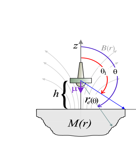
Figure 3: A finite base is parametrized by $r_{e}(\theta)$-the radial distance to the boundary for a given $\theta$. Integration in $r$ is carried out from $r=-h/\cos\theta$ to $r_{e}\left(\theta\right)$. The polar angle of the upper-right corner of the base is $\theta_{1}$.

The upward force Eq.(7), which in this case is given by setting

$${\mathbf{M(r)}}=M_{0}{\mathbf{\hat{n}}(\theta),}$$

is obtained from

$$\dfrac{1}{M_{0}}\dfrac{4\pi}{\mu_{0}}\left.\dfrac{\partial B_{z}}{\partial z}\right|_{z=h} =-6\pi{\displaystyle\int\limits_{\theta_{1}}^{\pi}}d\theta\sin\theta\sqrt{4\cos^{4}\theta+\sin^{4}\theta}$$ (15)

$$\times\left(-\frac{1}{r_{e}(\theta)}-\dfrac{\cos\theta}{h}\right).$$

According to the Lagrange’s multipliers method [13], the target function that is to be maximized is

$$T\equiv\frac{1}{M_{0}}\dfrac{4\pi}{\mu_{0}}\left.\dfrac{\partial B_{z}}{\partial z}\right|_{z=h}-\frac{1}{\lambda^{4}}\left(V_{0}-V\right),$$ (16)

where $1/\lambda^{4}$ is the Lagrange’s multiplier and $V_{0}$ is the given volume of the base. The target function is a functional of $r_{e}(\theta)$. We require that a variation of $T$ with respect to $r_{e}(\theta)$ would vanish, thus

$$\frac{\delta T}{\delta r_{e}(\theta)}=\frac{1}{M_{0}}\dfrac{4\pi}{\mu_{0}}\frac{\delta}{\delta r_{e}(\theta)}\left[\left.\dfrac{\partial B_{z}}{\partial z}\right|_{z=h}\right]+\frac{1}{\lambda^{4}}\frac{\delta V}{\delta r_{e}(\theta)}=0.$$ (17)

Using Eqs.(14),(15) we find that

$$\frac{\delta T}{\delta r_{e}(\theta)}=2\pi{\displaystyle\int\limits_{\theta_{1}}^{\pi}}d\theta\sin\theta\left\{-\frac{3\sqrt{4\cos^{4}\theta+\sin^{4}\theta}}{r_{e}^{2}(\theta)}+\frac{r_{e}^{2}(\theta)}{\lambda^{4}}\right\}\text{.}$$ (18)

Therefore, the required parametrization $r_{e}(\theta)$ is obtained by equating the integrand in Eq.(18) to zero, giving

$$\frac{r_{e}(\theta)}{\lambda}=\left[3\sqrt{4\cos^{4}\theta+\sin^{4}\theta}\right]^{1/4}.$$ (19)

Eq.(19) defines the shape of the optimal base. We see that it is universal in the sense that as $V_{0}$ is changed, the optimal new plate’s shape is only a scaled version of the original one. Recall however, that $\theta_{1}$ is different.

The value of $\theta_{1}$, determined by Eq.(14), may be combined with Eq.(19) to read

$$\frac{h}{\lambda}=-\cos\theta_{1}\left[3\sqrt{4\cos^{4}\theta_{1}+\sin^{4}\theta_{1}}\right]^{1/4}=f^{-1}\left(\theta_{1}\right),$$ (20)

which implicitly expresses $\theta_{1}$ in terms of $h/\lambda$. We denote this function by $f(x)$, and write

$$\theta_{1}=f(h/\lambda)\text{.}$$

In addition, we use Eq.(19) to arrive to an explicit expression for the volume $V_{0}$, given in Eq.(13):

$$\dfrac{V_{0}}{\lambda^{3}}=G(h/\lambda),$$

where

$$G\left(x\right)\equiv\dfrac{2\pi}{3}{\displaystyle\int\limits_{\theta_{1}=f(x)}^{\pi}}d\theta\sin\theta\left(\begin{array}[c]{c}\left[3\sqrt{4\cos^{4}\theta+\sin^{4}\theta}\right]^{3/4}\\ +\dfrac{x^{3}}{\cos^{3}\theta}\end{array}\right)\text{.}$$

Similarly, applying Eq.(19) to Eq.(15) yields

$$\left.\dfrac{\partial B_{z}}{\partial z}\right|_{z=h}\lambda=-M_{0}S(h/\lambda)$$ (21)

with the definition

$$S(x) \equiv 6\pi{\displaystyle\int\limits_{\theta_{1}=f(x)}^{\pi}}d\theta\sin\theta\sqrt{4\cos^{4}\theta+\sin^{4}\theta}$$

$$\times\left[\dfrac{-1}{\left(3\sqrt{4\cos^{4}\theta+\sin^{4}\theta}\right)^{1/4}}-\dfrac{\cos\theta}{x}\right]\text{.}$$

Using Eq.(21) with the equilibrium condition Eq.(4), we find that

$$\frac{\lambda}{l_{0}}=S(h/\lambda),$$ (22)

and with few more steps we arrive to

$$\begin{array}[c]{c}\dfrac{h}{l_{0}}=\dfrac{h}{\lambda}S\left(\dfrac{h}{\lambda}\right),\\ \dfrac{V_{0}}{l_{0}^{3}}=G\left(\dfrac{h}{\lambda}\right)S^{3}\left(\dfrac{h}{\lambda}\right).\end{array}$$ (23)

We see that $h/l_{0}$ depends on $V_{0}/l_{0}^{3}$ through an intermediate variable $h/\lambda$. It can be solved numerically by “running” over a wide range of $h/\lambda$ and evaluating $h/l_{0}$ and $V_{0}/l_{0}^{3}$ for each of its values. The result is given by the dash-dotted line in Fig.(6).

Note that at the limit $V_{0}\rightarrow\infty$ we find that $h=12l_{0}$, in agreement with the result of section(II-B). The asymptotic behavior of $h$ as $V_{0}\rightarrow 0$ is quite interesting also: This limit may be evaluated from the above equations but it is much simpler (and more instructive) to use the following argument: At the low volume limit, the base may be considered as a dipole centered at the origin. Such an assumption is valid only if $(h/l_{0})^{3}\gg V_{0}/l_{0}^{3}$. In this case it is easy to see that the magnetic force, acting on the top, is just

$$\left.\dfrac{\partial B_{z}}{\partial z}\right|_{z=h}=-\dfrac{\mu_{0}}{4\pi}\dfrac{6M_{0}V_{0}}{h^{4}},$$

and hence

$$-\mu\left.\dfrac{\partial B_{z}}{\partial z}\right|_{z=h}=\dfrac{\mu_{0}}{4\pi}\mu\dfrac{6M_{0}V_{0}}{h^{4}}=mg.$$

Using the definition of $l_{0}$ we may rewrite the last result as

$$\dfrac{h}{l_{0}}=\left[6\dfrac{V_{0}}{l_{0}^{3}}\right]^{1/4}.$$

We thus conclude that

$$\lim\limits_{V_{0}/l_{0}^{3}\rightarrow 0}\left(\dfrac{h}{l_{0}}\right)\rightarrow\left[6\dfrac{V_{0}}{l_{0}^{3}}\right]^{1/4}.$$ (24)

Note that since

$$\lim_{V_{0}/l_{0}^{3}\rightarrow 0}\dfrac{V_{0}/l_{0}^{3}}{(h/l_{0})^{3}}\sim\left(\frac{V_{0}}{l_{0}^{3}}\right)^{1/4}=0,$$

we see that our assumption is confirmed. The asymptotic line of Eq.(24) is also plotted in Fig.(6) by the dash-dot-dotted line. It is conspicuous that it is indeed an asymptotic.

II-E Uniformly magnetized, finite base.

The solution for this case is essentially similar to the solution presented in the previous section. The only difference is in the form of the magnetization that is used. Here we take ${\mathbf{M(r)}}=M_{0}{\mathbf{\hat{z}}}$ instead of ${\mathbf{M(r)}}=M_{0}{\mathbf{\hat{n}}}(\theta)$. The relation between $h/l_{0}$ and $V_{0}/l_{0}^{3}$ is again given by Eqs.(23) with the following new definitions:

$$\begin{array}[c]{c}f^{-1}(\theta)\equiv\cos\theta\left[3\cos\theta\left(5\sin^{2}\theta-2\right)\right]^{1/4},\\ G(x)\equiv\dfrac{2\pi}{3}{\displaystyle\int\limits_{f(x)}^{\pi}}d\theta\sin\theta\left(\begin{array}[c]{c}\left[3\cos\theta\left(5\sin^{2}\theta-2\right)\right]^{3/4}\\ +\dfrac{x^{3}}{\cos^{3}\theta}\end{array}\right),\\ S(x)\equiv 6\pi{\displaystyle\int\limits_{f(x)}^{\pi}}d\theta\sin\theta\cos\theta\left(5\sin^{2}\theta-2\right)\\ \times\left[\dfrac{-1}{\left[3\cos\theta\left(5\sin^{2}\theta-2\right)\right]^{1/4}}-\dfrac{\cos\theta}{x}\right].\end{array}$$

The result of this calculation is given by the dotted line in Fig.(6). Note that in this case $h\rightarrow 3.5l_{0}$ as $V_{0}\rightarrow\infty$, which is again in agreement with the result of section(II-C). The asymptotic behavior of $h$ as $V_{0}\rightarrow 0$ is identical to the result that was found in the previous section.

II-F Uniformly magnetized, finite, cylindrical base and stability.

In this case we take the base to be a uniformly magnetized cylinder with a magnetization ${\mathbf{M(r)}}=M_{0}{\mathbf{\hat{z}}}$. The radius of the cylinder is $R$ and its thickness is $d$, with its upper base at the $z=0$ plane, as is shown in Fig.(4).

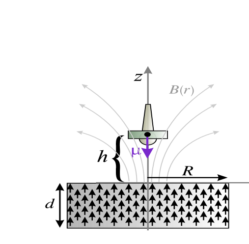
Figure 4: The top hovers stably over a cylindrical base of radius $R$, thickness $d$, and vertical magnetization $M_{0}$.

The magnetic field outside the cylinder is essentially the field outside a solenoid with similar dimensions. Thus, the $z$-component of the magnetic field along the $z$-axis is given by[14]:

$$B_{z}(z)=\dfrac{\mu_{0}}{4\pi}M_{0}W\left(\dfrac{z}{R};\dfrac{d}{R}\right),$$ (25)

where

$$W\left(x,y\right)\equiv 2\pi\left[\dfrac{x}{\sqrt{x^{2}+1}}-\dfrac{x+y}{\sqrt{(x+y)^{2}+1}}\right]\text{.}$$

We also define the function $F(x,y)$, to be used later, as

$$F(x,y)\equiv-\dfrac{\partial W\left(x,y\right)}{\partial x}\text{.}$$

We now formulate the conditions for the stability of the spinning top against both axial and lateral translations: Stability in the $z$-direction is determined by the sign of the ‘spring-constant’ in that direction – $k_{z}$. Under the adiabatic approximation, the latter is given by the curvature of the effective energy along that direction. Hence,

$$k_{z}\equiv\left.\dfrac{\partial^{2}E_{\text{eff}}}{\partial z^{2}}\right|_{\begin{subarray}{c}z=h\\ \rho=0\end{subarray}}=\mu\left.\frac{\partial^{2}\left|\mathbf{B}\right|}{\partial z^{2}}\right|_{\begin{subarray}{c}z=h\\ \rho=0\end{subarray}}=\mu\left.\frac{\partial^{2}B_{z}}{\partial z^{2}}\right|_{z=h},$$ (26)

where $\rho$ is the radial distance, in cylindrical coordinate system, from the $z$-axis.

Similarly, stability in the lateral direction $\hat{\rho}$, is governed by the sign of

$$k_{\rho} \equiv\left.\dfrac{\partial^{2}E_{\text{eff}}}{\partial\rho^{2}}\right|_{\begin{subarray}{c}z=h\\ \rho=0\end{subarray}}=\mu\left.\frac{\partial^{2}\left|\mathbf{B}\right|}{\partial\rho^{2}}\right|_{\begin{subarray}{c}z=h\\ \rho=0\end{subarray}}$$ (27)

$$=\mu\left[\frac{1}{4\left.B_{z}\right|_{z=h}}\left(\left.\frac{\partial B_{z}}{\partial z}\right|_{z=h}\right)^{2}-\frac{1}{2}\left.\frac{\partial^{2}B_{z}}{\partial z^{2}}\right|_{z=h}\right],$$

where in the last equality use has been made of the cylindrical symmetry of the magnetic field and the fact that $B_{z}$ and all of its Cartesian derivatives are Harmonic functions [15].

For the spinning top to be stable against translations, both $k_{z}$ and $k_{\rho}$ should be positive. Comparing Eq.(27) to Eq.(26), we see that when $B_{z}\rightarrow\infty$, then $k_{\rho}$ $\rightarrow-$ $k_{z}/2$, and therefore one of the pair $(k_{z}$,$k_{\rho})$ must be negative. Thus, when the magnetic field diverges at a point, a top placed at that point cannot be stable. This proves that the highest hovering height, found in Section (II-B), is not under stable conditions.

The restriction that both $k_{z}$ and $k_{\rho}$ should be positive defines a stable region along the $z$ axis. As an example it can be shown [9], that for a base in the shape of a thin disk of radius $R_{d}$, the value of $k_{z}$ is positive whenever $z>R_{d}/2$, whereas $k_{\rho}$ is positive for $z<\sqrt{2/5}R_{d}$. The region of stability in this case is therefore $R_{d}/2<z<\sqrt{2/5}R_{d}$. Within that region there exists a point $z_{i}$ for which $k_{z}=k_{\rho}$. In the case of the disk it is $z_{i}=\sqrt{2/7}R_{d}$. We call this point the isotropically stable point because the restoring (stabilizing) force which acts on a top, which is tuned to hover at $h=z_{i}$ is isotropic, depending only on the deviation from the equilibrium position and not on its direction.

For a general cylinder we now consider two distinct situations: The first is the one in which the stable point is isotropic, i.e. a hovering height $h$ for which $k_{\rho}=k_{z}$. The second is the case where $h$ is at the verge of stability in the lateral direction. This is also the highest stable point, characterized by $k_{\rho}=0$. Using Eqs.(26),(27) we write each of the two distinct conditions as

$$\frac{1}{\left.B_{z}\right|_{z=h}}\left(\left.\frac{\partial B_{z}}{\partial z}\right|_{z=h}\right)^{2}=a\left.\frac{\partial^{2}B_{z}}{\partial z^{2}}\right|_{z=h},$$ (28)

where $a=6$ for the first situation and $a=2$ for the second.

Substituting Eq.(25) into Eq.(28) defines a functional relationship between $h/R$ and $d/R$ denoted by the function $G()$,

$$\frac{h}{R}\equiv G\left(d/R\right).$$

Differentiating Eq.(25) with respect to $z$, setting $z=h$, and using the equilibrium condition Eq.(4), gives

$$\frac{R}{l_{0}}=F\left(h/R;d/R\right)=N\left(d/R\right),$$

where

$$N(y)\equiv F(G(y),y)\text{.}$$

Combining it with an expression for the volume, gives

$$\begin{array}[c]{c}\dfrac{V_{0}}{l_{0}^{3}}=\dfrac{\pi R^{2}d}{l_{0}^{3}}=\pi\left(\dfrac{d}{R}\right)\left(\dfrac{R}{l_{0}}\right)^{3}=\pi\dfrac{d}{R}N^{3}\left(d/R\right),\\ \dfrac{h}{l_{0}}=\dfrac{h}{R}\dfrac{R}{l_{0}}=G(d/R)N\left(d/R\right),\end{array}$$ (29)

which expresses the volume $V_{0}$ and the levitation height $h$ in terms of a common variable $d/R$. Running over $d/R$, and evaluating the volume and height according to Eqs.(29), furnishes the required relation between $h/l_{0}$ and $V_{0}/l_{0}^{3}$. This plot is shown in Fig.(6) where the solid line corresponds to $a=2$ (the isotropic case) and the dotted line corresponds to $a=6$ (the highest stable point).

Note that both of these plots are not monotonically increasing. They possess a maximum of $h$ at some optimal volume $V_{opt}$. For $a=6$ we find that $h_{\max}\simeq 1.3l_{0}$ and $V_{opt}\simeq 310l_{0}^{3}$, whereas for $a=2$ these are $h_{\max}\simeq 0.88l_{0}$ and $V_{opt}\simeq 90l_{0}^{3}$. This indicates that using too a much material worsen the largest height that can be achieved, which is reminiscent of our conclusion of Sec.(II-C). If the given volume is larger than $V_{opt}$ however, we can always use only an amount of volume equal to $V_{opt}$ and discard the rest of the material. Hence, in principal at least, one can realize the largest possible height, which is why the plots of $h$ vs. $V_{0}$ had been artificially corrected by assigning the maximum value of $h$ for the values of $V_{0}$ that are larger than $V_{opt}$.

II-G Infinite,arbitrarily magnetized base and stability.

In this last section we consider the case of an infinite base, which may be arbitrarily magnetized, such that the height of levitation is maximized, yet the top is stable against both axial and lateral translations. In order to solve this problem, one needs to maximize the magnetic force $\partial B_{z}/\partial z$ under the constraints that $k_{z}$ and $k_{\rho}$, defined in Eqs.(26) and (27) respectively, are both positive. The last requirement however, results in a non-linear inequality, which cannot be solved analytically. The method we take here is to use the constraint $k_{z}\propto\partial^{2}B_{z}/\partial z^{2}=0$ instead, which marks the lower end of the stability region along the $z$-axis.

Consider an infinitesimal magnetic dipole at the point $(r,\theta)$ within the base with magnetization $M_{0}$. It is situated below the expected hovering position, as is shown in Fig.(5), and its direction makes an angle $\alpha(r,\theta)$ with the line joining the dipole to the equilibrium position of the top.

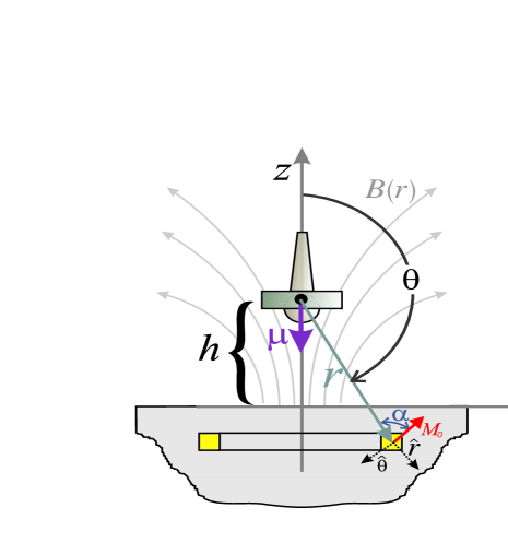
Figure 5: The magnetization density at point $(r,\theta)$ is $M_{0}$ and its direction makes an angle $\alpha\left(r,\theta\right)$ with the unit vector $\mathbf{\hat{r}}$. The angle distribution-$\alpha\left(r,\theta\right)$ is chosen so as to maximize the levitation height while maintaining the translational stability of the top.

Substituting

$${\mathbf{M}}=-\sin\alpha\left(r,\theta\right){\mathbf{\hat{\theta}}}-\cos\alpha\left(r,\theta\right){\mathbf{\hat{r}},}$$

into Eqs.(7),(9), gives

$$\left.\dfrac{\partial B_{z}}{\partial z}\right|_{z=h} =M_{0}\dfrac{\mu_{0}}{4\pi}\int\limits_{\pi/2}^{\pi}d\theta\sin\theta{\displaystyle\int\limits_{-h/\cos(\theta)}^{\infty}}dr\dfrac{2\pi r^{2}}{r^{4}}$$ (30)

$$\times\left\{\begin{array}[c]{c}-6\sin\alpha\sin\theta\cos\theta\\ -3(3\cos^{2}\theta-1)\cos\alpha\end{array}\right\},$$ (33)

and

$$\left.\dfrac{\partial^{2}B_{z}}{\partial z^{2}}\right|_{z=h} =M_{0}\dfrac{\mu_{0}}{4\pi}\int\limits_{\pi/2}^{\pi}d\theta\sin\theta{\displaystyle\int\limits_{-h/\cos(\theta)}^{\infty}}dr\dfrac{2\pi r^{2}}{r^{5}}$$ (34)

$$\times\left\{\begin{array}[c]{c}-9\sin\theta\left(5\cos^{2}\theta-1\right)\sin\alpha\\ -12\cos\theta(5\cos^{2}\theta-3)\cos\alpha\end{array}\right\}.$$ (37)

The target function to be extremized in this case, is given by

$$T\left[\alpha(r,\theta)\right]=\left.\frac{\partial B_{z}}{\partial z}\right|_{z=h}+\lambda\left.\dfrac{\partial^{2}B_{z}}{\partial z^{2}}\right|_{z=h},$$ (38)

and is a functional of $\alpha(r,\theta)$, with $\lambda$ being the Lagrange’s multiplier. Since the variation of $T$ with respect to $\alpha(r,\theta)$ must vanish, we find, on substitution of Eqs.(30) and (34) into Eq. (38), that $\alpha(r,\theta)$ is given by

$$\tan\alpha(r,\theta)=\frac{2\sin\theta\cos\theta+3\dfrac{\lambda}{r}\sin\theta\left(5\cos^{2}\theta-1\right)}{(3\cos^{2}\theta-1)+4\dfrac{\lambda}{r}\cos\theta(5\cos^{2}\theta-3)}\text{.}$$ (39)

Using Eq.(39) inside Eq.(34), and requiring that $\partial^{2}B_{z}/\partial z^{2}=0$, gives the equation for $\lambda/h$

$$\int\limits_{\pi/2}^{\pi}d\theta\sin(\theta){\displaystyle\int\limits_{0}^{-\cos(\theta)}}ydy\left\{\begin{array}[c]{c}3\sin\theta\left(5\cos^{2}\theta-1\right)\sin\alpha\\ +4\cos\theta(5\cos^{2}\theta-3)\cos\alpha\end{array}\right\}=0\text{,}$$ (40)

in which $\alpha(r,\theta)$ depends on $y$ according to

$$\tan\alpha(r,\theta)=\frac{2\sin\theta\cos\theta+3\dfrac{\lambda}{h}y\sin\theta\left(5\cos^{2}\theta-1\right)}{(3\cos^{2}\theta-1)+4\dfrac{\lambda}{h}y\cos\theta(5\cos^{2}\theta-3)}.$$

Note that in Eq.(40) the variable $r$ has been changed to $y=h/r$. This way the double integration is finite and the singularity in the integrand is eliminated.

The numerical solution of Eq.(40) gives

$$\lambda=0.424h.$$

Using this value inside Eq.(30) yields

$$\left.\frac{\partial B_{z}}{\partial z}\right|_{z=h}=-1.33\dfrac{\mu_{0}}{4\pi}\frac{2\pi M_{0}}{h},$$ (41)

which, together with the equilibrium condition, gives

$$h_{\max}\simeq 8.4\dfrac{\mu_{0}}{4\pi}\frac{M_{0}\mu}{mg}=8.4l_{0}.$$ (42)

Note that, though the gradient of the field is finite, the field itself diverges, and hence $k_{\rho}=-k_{z}/2$. As $k_{z}=0$ in the case we studied here, we conclude that $k_{\rho}$ also vanishes. Thus, the lowest stable hovering height and the highest one coincide, leaving no range of stability. A small relaxation in the conditions however, such as limiting the volume of the material to a finite, though very large value, results in a formation of a finite albeit small, range of stability.

III Discussion.

We showed that the maximum levitation height of the U-CAS is bounded and is given in terms of a characteristic length $l_{0}$, which depends on the properties of the substance that the base and the top are made of. Note also, that $\mu/m=M_{0}^{top}/\rho$ where $\rho$ is the mass density of the top, and $M_{0}^{top}$ is its magnetization density. Since $M_{0}\simeq B_{r}/\mu_{0}$, where $B_{r}$ is the residual induction, and since $B_{r}$ is related to the energy product [16] via $(BH)_{\text{max}}\simeq B_{r}^{2}/4\mu_{0}$, we may also write $l_{0}$ as

$$l_{0}=\dfrac{\mu_{0}}{4\pi}\dfrac{M_{0}^{top}M_{0}^{base}}{\rho g}\simeq\dfrac{1}{\pi}\dfrac{\sqrt{(BH)_{\text{max}}^{top}(BH)_{\text{max}}^{base}}}{\rho g}\text{.}$$ (43)

In this form, $l_{0}$ can be easily estimated from the knowledge of the energy product of the material. The best candidates for large hovering heights are the Nd-Fe-B magnets. An example of which is Vacuumschmelze’s VACODYM 344 HR [17], whose remanence ($B_{r}$) is $13.5$ KGauss and whose density is $7.5$ gr/cm³. For this magnet, the magnetization is $M=B_{r}/4\pi=1070$ emu/cm³. Thus, with $g=980$ cm/sec², we find that $l_{0}\simeq 1.6$ meter. This gives, according to Eq.(42), a maximum stable hovering height of about $13$ meters!. Typical values of the energy product, density and corresponding $l_{0}$, for modern commercial magnets available today are listed in Table I.

Base		Top			$l_{0}$[m]
material	($BH$)${}_{\text{max}}$[19]	material	($BH$)${}_{\text{max}}$[19]	$\rho$[Kg/m3]
Fe-Nd-B	$320$[KJ/m3]	Fe-Nd-B	$320$[KJ/m3]	$7500$	$1.35$
Ferrite	$32$[KJ/m3]	Fe-Nd-B	$320$[KJ/m3]	$7500$	$0.43$
Strnat[19]	$800$[KJ/m3]	Strnat[19]	$800$[KJ/m3]	$8000$	$3.2$

TABLE I: The value of $l_{0}$ for different base-top material combinations.

According to Eq.(43) the characteristic length is proportional to the energy product. Therefore, the larger the energy product is, the larger $l_{0}$ will be. A question is then asked: what is the highest conceivable energy product? This question has been already discussed by Strnat [18], according to which “ …it seems reasonable to assume that the best room-temperature energy products will never exceed $\sim 100$ MGOe”, which is about $8\cdot 10^{5}$ Joules/m³, and is also included in Table I. These predictions, however, assume that a way might be found to give a fairly high $H_{ci}$ to any magnetic material.

Table II summarizes the upper and lower bounds for the maximum hovering height under a selected number of constraints.

Constraints	Lower bound	Upper bound
None	$1.3l_{0}$	$12l_{0}$
U	$1.3l_{0}$	$3.5l_{0}$
S	$1.3l_{0}$	$8.4l_{0}$
U and S	$1.3l_{0}$	$3.5l_{0}$
V	Fig.(6)	Fig.(6)

TABLE II: Summary of the bounds for the maximum levitation height of the U-CAS under various constraints: U=Uniformly magnetized base plate , S=stable hovering, V=under a given Volume

It is important to note, that in the above derivation we assumed that the magnetization vector ${\mathbf{M}}(r,\theta)$ is independent of the field. Though this is a very good approximation for modern permanent magnets like rare-earth magnets, its only an approximation even for these. Furthermore, the maximum field at the top is limited by its mechanical and magnetic strength: Stability considerations show [21] that the spinning speed of the top while hovering must be greater than $\sqrt{\mu\left.B_{z}\right|_{z=h}/(I_{3}-I_{1})}$ where $I_{3}$ and $I_{1}$ are the moments of inertia along the principal and secondary axes, respectively. Also, the maximum field at the top is limited by its coercivity as the field is opposite to the magnetization. Thus, in practice, Eq.(42) should be considered as an upper bound for the maximum hovering height of the U-CAS.

Yet another way to increase the hovering height of the top is to use current coil for the base, instead of a permanent magnet [7]. The advantage of the coil over the magnetic plate is in the fact that one can raise the top to the levitation point by electrical means instead of raising the top mechanically, as in the permanent magnet case. Here, the hovering height is not limited directly by the strength of the magnetic field, but rather by the amount of power that one can deliver into the coil to overcome electrical resistance. One might argue that the use of superconducting wires for the coil should lift this constraint, but the hovering height is bounded in this case as well, for if the field increases beyond a critical value, the superconductor goes into its normal phase. We have shown [7], that for a given height of levitation $h$, the minimum power required for levitation is given by

$$P=A\frac{rg^{2}h^{3}}{\mu_{m}^{2}}\text{.}$$

Here, $P$ is the power in Watts, $r$ is the resistivity in $\Omega\cdot$cm, $g$ is the free-fall acceleration in cm$\cdot$sec^-1, $\mu_{m}$ is the magnetization per unit mass of the top in emu/gr, and $A$ is a number of dimensions Amp²emu²/erg²cm², and is determined by the shape and current distribution of the coil. We found that for a rectangular cross-section coil, the minimal value of $A\simeq 2300$. For the optimal coil however, we find that $A\simeq 490$.

IV Acknowledgments.

The authors thank Profs. M. Milgrom and M. Kugler for helpful discussions, and S. Tozik and N. Fernik for help in the calculations. One of the authors (S. S.) thanks RIKEN, Saitama in Japan and in particular Dr. Y. Kawamura for kindly hosting him during a short stay in Japan that triggered this study, as it is then that he became acquainted with the U-CAS.

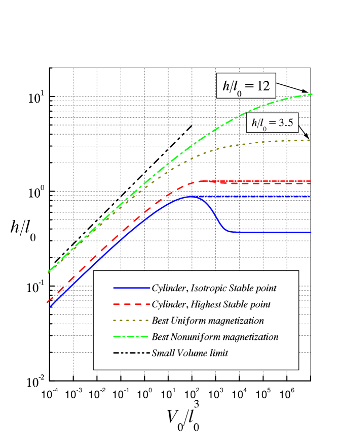
Figure 6: Bounds on the maximum levitation height Vs. volume for: Best magnetization possible (dash-dot line), Best uniform magnetization (dotted line), Uniformly magnetized cylinder with highest stable point (dashed line), Uniformly magnetized cylinder with isotropic stable point (solid line) and small volume limit (dash-dot-dot line). The two curves that correspond to the uniformly magnetized cylinder has been artificially corrected by extending the highest levitation point to higher volumes.

References

- [1] The U-CAS is available from Masudaya International Inc., 6-4, Kuramae, 2-Chome, Taito-Ku, Tokyo, 111 Japan.
- [2] The Levitron is available from ‘Fascinations’, 18964 Des Moines Way South, Seattle, WA 98148.
- [3] R. Harrigan, U.S. Patent Number: 4,382,245, Date of Patent: May 3, 1983.
- [4] Hones et al., U.S. Patent Number: 5,404,062, Date of Patent: Apr. 4, 1995.
- [5] T. Bergeman, G. Erez, H. J. Metcalf, “Magnetostatic trapping fields for neutral atoms”, Phys. Rev. A., vol. 35, no. 4, pp. 1535-1546, 1987.
- [6] M. V. Berry, “The levitron: An adiabatic trap for spin”, Proc. R. Soc. Lond. A, vol. 452, pp. 1207-1220, 1996.
- [7] S. Gov, H. Matzner and S. Shtrikman,“Hovering a magnetic top above an air coil”, Bulletin of the Israel Physical Society, vol. 42, pp. 121, 1996.
- [8] M. D. Simon, L. O. Heflinger and S. L. Ridgway, “Spin stabilized magnetic levitation”, Am. J. Phys. vol. 65, no. 4, pp. 286-292, 1997.
- [9] S. Gov, S. Shtrikman and H. Thomas, “On the dynamical stability of the hovering magnetic top”, accepted for publication in Physica D. A copy may be found in http://xxx.lanl.gov/abs/physics/9803020.
- [10] S. Gov, H. Matzner and S. Shtrikman, “Mass and tilt tolerances for magnetic top levitation”, Bulletin of the Israel Physical Society, vol. 44, pp. 81, 1998.
- [11] S. Gov, H. Matzner and S. Shtrikman, “Levitating a magnetic top above a vertically magnetized ring”, Bulletin of the Israel Physical Society, vol. 43, pp. 47, 1997.
- [12] Note that may be computed analytically with the result: . In this paper we are only interested in the numerical result which is .
- [13] R. Weinstock, “Calculus of Variations”, Dover books, Ch. 4, pp. 48.
- [14] E. M. Purcell, “Electricity and Magnetism”, second edition, Berkeley Physics Course, vol. 2, ch. 6, sec. 5, pp. 226–231.
- [15] J. D. Jackson, “Classical Electrodynamics”, 2 edition, John Wiley & sons, New York, 1975, ch. 5, sec. 9, pp. 191-194.
- [16] R. J. Parker, “Advances in Permanent Magnetism”, John Wiley & sons, New York, 1990, pp. 86.
- [17] Vacuumschmelze GMBH P.O.B. 2253 D-63412 Hanau Grüner Weg 37 D-63450 Hanau.
- [18] K. J. Strnat, “Modern Permanent Magnets for Application in Electro-Technology”, Proc. of the IEEE, vol. 78, no. 6, pp. 944-945, June 1990.
- [19] K. J. Strnat, “Modern Permanent Magnets for Application in Electro-Technology”, Proc. of the IEEE, vol. 78, no. 6, pp. 934, June 1990.
- [20] R. J. Parker, “Advances in Permanent Magnetism”, John Wiley & sons, New York, 1990, pp. 38.
- [21] P. Flanders, S. Gov, S. Shtrikman and H. Thomas, “On the spinning motion of the hovering magnetic top”, accepted for publication in Physica D. A copy may be found in http://xxx.lanl.gov/abs/physics/9803044.