How to quantify deterministic and random influences on the statistics of the foreign exchange market

Abstract

It is shown that prize changes of the US dollar - German Mark exchange rates upon different delay times can be regarded as a stochastic Marcovian process. Furthermore we show that from the empirical data the Kramers-Moyal coefficients can be estimated. Finally, we present an explicite Fokker-Planck equation which models very precisely the empirical probabilitiy distributions.

PACS: 02.50-r;05.10G

Since high-frequency intra-day data are available and easy to access, research on the dynamics of financial markets is enjoying a broad interest. [1, 2, 3, 4, 5, 6, 7]. Well-founded quantitative investigations now seem to be feasible. The identification of the underlying process leading to heavy tailed probability density function (pdf) of price changes and the volatility clustering (see fig.1) are of special interest. The shape of the pdf expresses an unexpected high probability of large price changes on short time scales which is of utmost importance for risk analysis. In a recent work [8], an analogy between the short-time dynamics of foreign exchange (FX) market and hydrodynamic turbulence has been proposed. This analogy postulates the existence of hierarchical features like a cascade process from large to small time scales in the dynamics of prices, similar to the energy cascade in turbulence c.f. [9]. This postulate has been supported by some work [7] and questioned by others [6].

One main claim of the hypothesis of cascade processes is that the statistics of the time series of the financial market can be determined. The aim of the present paper is to discuss a new kind of analysis capable to derive the underlying mathematical model directly from the given data. This method yields an estimation of an effective stochastic equation in the form of a Fokker-Planck equation (also known as Kolmogorov equation). The solutions of this equation yields the probability distributions with sufficient accuracy (see fig. 1). This means that our method is not based on the conventional phenomenological comparison between models and several stochastic aspects of financial data. Our approach demonstrates how multiplicative noise and deterministic forces interact leading to the heavy tailed statistics. [10]

Recently it has been demonstrated that from experimental data of turbulent flow the hierarchical features induced by the energy cascade can be extracted in form of a Fokker-Planck equation for the length scale dependence of velocity fluctuations [12]. In the following it will be shown the dynamics of foreign exchange rates can also be described by a Fokker-Planck equation. Here we use a data set consisting of 1,472,241 quotes for US dollar-German mark exchange rates from the years 1992 and 1993 as used in reference [8].

We investigate the statistical dependence of prize changes $\Delta x_{i}:=x(t+\Delta t_{i})-x(t)$ upon the delay time $\Delta t_{i}$. Here $x(t)$ denotes the exchange rate at time t. We will show that the prize changes $\Delta x_{1}$, $\Delta x_{2}$ for two delay times $\Delta t_{1}$, $\Delta t_{2}$ are statistically dependent, provided the difference $\Delta t_{2}-\Delta t_{1}$ is not too large and that the shorter time interval is nested inside the longer one.

In order to characterize the statistical dependency of price changes $\Delta x_{i}$, we have evaluated the joint probability density functions

$$p(\Delta x_{2},\Delta t_{2};\Delta x_{1},\Delta t_{1})$$ (1)

for various time delays $\Delta t_{2}<\Delta t_{1}$ directly from the given data set. One example of a contourplot of the logarithms of these functions is exhibited in figure 2. If the two price changes $\Delta x_{1}$, $\Delta x_{2}$ were statistically independent, the joint pdf would factorize into a product of two probability density functions:

$$p(\Delta x_{2},\Delta t_{2};\Delta x_{1},\Delta t_{1})=p(\Delta x_{2},\Delta t_{2})p(\Delta x_{1},\Delta t_{1}).$$ (2)

The tilted form of the probability density $p(\Delta x_{2},\Delta t_{2};\Delta x_{1},\Delta t_{1})$ clearly shows that such a factorization does not hold and that the two price changes are statistically dependent. This dependency is in accordance with observations of Müller et al. for cross-correlation functions of the same data [5]. To analyze these correlations in more detail, we address the question: What kind of statistical process underlies the price changes over a series of nested time delays $\Delta t_{i}$ of decreasing length? In general, a complete characterization of the statistical properties of the data set requires the evaluation of joint pdfs $p^{N}(\Delta x_{1},\Delta t_{1};....;\Delta x_{N},\Delta t_{N})$ depending on $N$ variables (for arbitrarily large $N$). In the case of a Markov process (a process without memory), an important simplification arises: The N-point pdf $p^{N}$ are generated by a product of the conditional probabilities $p(\Delta x_{i+1},\Delta t_{i+1}|\Delta x_{i},\Delta t_{i})$, for $i=1,...,N-1$. As a necessary condition, the Chapman-Kolmogorov equation [13]

$$p(\Delta x_{2},\Delta t_{2}|\Delta x_{1},\Delta t_{1})=\int\hbox{d}(\Delta x_{i})\,p(\Delta x_{2},\Delta t_{2}|\Delta x_{i},\Delta t_{i})\,p(\Delta x_{i},\Delta t_{i}|\Delta x_{1},\Delta t_{1})$$ (3)

should hold for any value of $\Delta t_{i}$ embedded in the interval

$$\Delta t_{2}<\Delta t_{3}<\Delta t_{1}\qquad.$$ (4)

We checked the validity of the Chapman-Kolmogorov equation for different $\Delta t_{i}$ triplets by comparing the directly evaluated conditional probability distributions $p(\Delta x_{2},\Delta t_{2}|\Delta x_{1},\Delta t_{1})$ with the ones calculated ($p_{cal}$) according to (3). In figure 3, the contour lines of the two corresponding pdfs are superimposed for the purpose of illustration; the red lines corresponding to $p_{cal}$. Only in the outer regions, there are visible deviations probably resulting from a finite resolution of the statistics.

As it is well-known, the Chapman-Kolmogorov [13] equation yields an evolution equation for the change of the distribution function $p(\Delta x,\Delta t)$ across the scales $\Delta t$.

For the following it is convenient (and without loss of generality) to consider a logarithmic time scale

$$\tau=-ln\Delta t\qquad.$$ (5)

Then, the limiting case $\Delta t\rightarrow 0$ corresponds to $\tau\rightarrow\infty$. The Chapman-Kolmogorov equation formulated in differential form yields a master equation, which can take the form of a Fokker-Planck equation (for a detailed discussion we refer the reader to [13]):

$$\frac{d}{d\tau_{2}}p(\Delta x,\tau)=[-\frac{\partial}{\partial\Delta x}D^{(1)}(\Delta x,\tau)+\frac{\partial^{2}}{\partial\Delta x^{2}}D^{(2)}(\Delta x,\tau)]p(\Delta x,\tau)$$ (6)

The drift and diffusion coefficients $D^{(1)}(\Delta x,\tau)$, $D^{(2)}(\Delta x,\tau)$ can be estimated directly from the data as moments $M^{(k)}$ of the conditional probability distributions (c.f fig. 3):

$$D^{(k)}(\Delta x,\tau) = \frac{1}{k!}lim_{\Delta\tau\rightarrow 0}M^{(k)}$$ (7)

$$M^{(k)} = \frac{1}{\Delta\tau}\int d\Delta x^{\prime}(\Delta x^{\prime}-\Delta x)^{k}p(\Delta x^{\prime},\tau+\Delta\tau|\Delta x,\tau).$$

As indicated by the functional $\Delta x$ dependency of the moments $M^{(k)}$, it turns out that the drift term $D^{(1)}$ is a linear function of $\Delta x$, whereas the diffusion term $D^{(2)}$ is a function quadratic in $\Delta x$. In fact, from a careful analysis of the data set we obtain the following approximation:

$$D^{(1)} = -0.44\Delta x$$

$$D^{(2)} = 0.003\exp{(-\tau/2)}+0.019(\Delta x+0.04)^{2}$$ (8)

($\Delta x$ is measured in units of the standard deviation of $\Delta x$ at $\Delta t=40960s$). With these coefficients we can solve the Fokker-Planck equation (6) for the pdf at times $\tau>\tau_{0}$ with a given distribution at $\tau_{0}$. Figure 1 shows that the solutions of our model nicely fit the experimentally determined pdf’s [14]. In contrast to the use of phenomenological supposed fitting functions c.f [8, 2], we obtained the changing forms of the pdfs by a differential equation. This method provides the evolution of pdfs from large time delays to smaller ones. This definitely is a new quality in describing the hierarchical structure of such data sets. At last, it is important to note that our finding of the Fokker-Planck equation for the cascade is in good agreement with the previously found phenomenological description in [8]. Based on the given exact solution of our Fokker-Planck equation [11], we see that the chosen type of fitting function for the pdfs in [8] was the correct one. Furthermore, we see that the observed quadratic dependency of the diffusion term $D^{2}$ corresponds to the found logarithmic scaling of the intermittency parameter in [8], which was taken as an essential point to propose the analogy between turbulence and the financial market.

We remind the reader that the Fokker-Planck equation is equivalent to a Langevin equation of the form (we use the Ito interpretation [13]):

$$\frac{d}{d\tau}\Delta x(\tau)=D^{(1)}(\Delta x(\tau),\tau)+\sqrt{D^{(2)}(\Delta x(\tau),\tau)}F(\tau)\qquad.$$ (9)

Here, $F(\tau)$ is a fluctuating force with gaussian statistics $\delta$-correlated in $\tau$:

$$<F(\tau)>=0\qquad,\qquad<F(\tau)F(\tau^{\prime})>=\delta(\tau-\tau^{\prime})$$ (10)

In our approximation (How to quantify deterministic and random influences on the statistics of the foreign exchange market) the stochastic process underlying the prize changes is a linear stochastic process with multiplicative noise, at least for large values of $\Delta x$:

$$\frac{d}{d\tau}\Delta x(\tau)=-0.44\Delta x(\tau)+\sqrt{.019}\Delta x(\tau)F(\tau)\qquad.$$ (11)

This stochastic equation yields realizations of prize changes $\Delta x(\tau)$, whose ensemble averages can be described by the probability distributions $p(\Delta x,\tau)$. Thus, the Langevin equation (9) produces the possibility to simulate the price cascades for time delays from about a day down to several minutes. Furthermore, with this last presentation of our results it becomes clear that we are able to separate the deterministic and the noisy influence on the hierarchical structure of the finance data in terms of the coefficients $D^{(1)}$ and $D^{(2)}$, respectively.

Summarizing, it is the concept of a cascade in time hierarchy that allowed us to derive the results of the present paper, which in turn quantitatively supports the initial concept of an analogy between turbulence and financial data. Furthermore, we have shown that the smooth evolution of the pdfs down along the cascade towards smaller time delays is caused by a Markov process with multiplicative noise.

Helpful discussions and the careful reading of our manuscript by Wolfgang Breymann, Shoaleh Ghashghai and Peter Talkner are acknowledged. The FX data set has been provided by Olsen & Associates (Zürich).

figure captions

Figure 1: Probability densities (pdf) $p(\Delta x,\Delta t)$ of the price changes $\Delta x=x(t+\Delta t)-x(t)$ for the time delays $\Delta t=5120,10240,20480,40960s$ (from bottom to top). Symbols: the results obtains from the analysis of middle prices of 1,472,241 bit-ask quotes for the US dollar-German Mark exchange rates from 1 October until 30 September 1993. Full lines: results form a numerical iteration of an effective Fokker-Planck equation with the initial condition of the probability distribution for $\Delta t=40960s$. As drift term $D^{(1)}=-0.44\Delta x$ and as diffusion term $D^{(2)}=0.003exp(-\tau/2)+0.019(\Delta x+0.04)^{2}$ were taken. The units of $\Delta x$ are multiples of the standard deviation $\sigma$ of $\Delta x$ with $\Delta t=40960s$. The pdfs are shifted in vertical directions for convenience of presentation.

Figure 2: Joint pdf $p(\Delta x_{2},\Delta t_{2};\Delta x_{1},\Delta t_{1})$ for the simultaneous occurrence of price differences $\Delta x_{1}(\Delta t_{1})$ and $\Delta x_{2}(\Delta t_{2})$ for US dollar-Deutsch mark exchange rates. The contour plot is shown for $\Delta t_{1}=6168s$ and $\Delta t_{2}=5120s$. $\sigma=0.0635DM$ denotes the standard deviation of $x(t)$. The contour lines correspond to $\log p=-1,\ldots,-4$. If the two price changes were statistically independent the joint pdf would factorize into a product of two pdfs: $p(\Delta x_{2},\Delta t_{2};\Delta x_{1},\Delta t_{1})=p(\Delta x_{2},\Delta t_{2})p(\Delta x_{1},\Delta t_{1})$. The tilted form of the joint pdf provides evidence that such a factorization does not appear for small values of $|\log(\Delta t_{1}/\Delta t_{2})|$.

Figure 3 : Contour plot of the conditional pdf $p(\Delta x_{2},\Delta t_{2}|\Delta x_{1},\Delta t_{1})=$ $p(\Delta x_{2},\Delta t_{2};\Delta x_{1},\Delta t_{1})/$ $p(\Delta x_{1},\Delta t_{1})$ for $\Delta t_{2}=\Delta t_{1}/(1.2)^{2}$ and $t_{1}=5120$, in the range ($-3\sigma\leq\Delta x_{i}\leq 3\sigma$, $i=1,2$). $\sigma$ denotes the standard deviation of $x(t)$, see fig.2. The contour lines correspond to $\log p=-1,\ldots,-4$. For statistically unrelated quantities the conditional pdf would reduce to the probability density $p(\Delta x_{2},\Delta t_{2})$.
In order to verify the Chapman-Kolmogorov equation, the directly evaluated pdf (black lines) is compared with the pdf calculated by $p_{cal}(\Delta x_{2},\Delta t_{2}|\Delta x_{1},\Delta t_{1})=\int dx_{i}p(\Delta x_{2},\Delta t_{2}|\Delta x_{i},\Delta t_{i})p(\Delta x_{i},\Delta t_{i}|\Delta x_{1},\Delta t_{1})$ for $\Delta t_{2}=\Delta t_{1}/(1.2)^{2};\Delta t_{i}=\Delta t_{1}/1.2$ (red lines). Assuming an statistical error of the square root of the number of events of each bin we find that both pdfs are statistically identical.

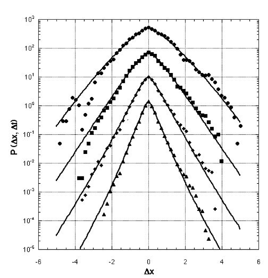
Figure 1:

Figure 2:

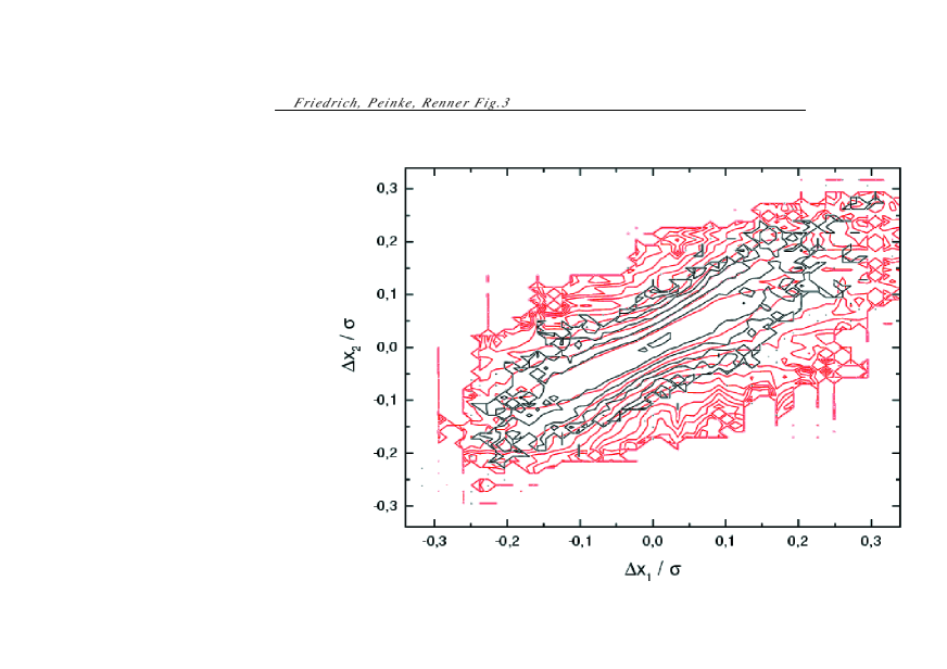
Figure 3:

References

- [1] Müller, U. A. et al. Journal of Banking and Finance 14, 1189–1208 (1990).
- [2] Mantegna, R. N., Stanley, H. E. Nature 376, 46–49 (1995).
- [3] Vassilicos, J. C. Nature 374, 408–409 (1995).
- [4] The 1st International Conference on High Frequency Data in finance, Olsen & Associates, Zürich, 1995).
- [5] Müller, U. A., et al., J. Empirical Fin. (in the press).
- [6] Mantegna, R. N. & Stanley, H.E. N., Nature 383, 587-588 (1996).
- [7] Beck, C. and Hilgers, Int. J. Bifurcation and Chaos, in press; Schmitt,F., Schertzer, D., Lovejoy,S. : Turbulence fluctuations in financial markets: a multifractal approach, in Chaos, Fractals and Models, G. Salvadori ed., Italian University Press, 1998. Arneodo, A., Muzy, J.-F., Sornette, D., Eur. Phys. J. B 2, 277-282 (1998).
- [8] Ghashghaie, S., Breymann, W., Peinke, J., Talkner, P., and Dodge, Y., Nature 381, 767-770 (1996).
- [9] Frisch, U.: Turbulence,(Cambridge ,1995).
- [10] Based on a recent work by Donkov et.al [11] it is easily seen that the obtained Fokker-Planck equation is consistent with the phenomenological results presented previously [8].
- [11] Donkov,A.A., Donkov, A.D., Grancharova, E.I., The exact Solution of one Fokker-Planck Type Equation …, math-ph/9807010.
- [12] Friedrich, R., Peinke, J., Physica D 102, 147 (1997); Friedrich, R., Peinke, J., Phys. Rev. Lett. 78, 863 (1997)
- [13] Risken, H., The Fokker-Planck equation, (Springer-Verlag Berlin, 1984); Hänggi, P. and Thomas, H., Physics Reports 88, 207 (1982); Van Kampen,N. G., Stochastic processes in physics and chemistry (North Holland, Amsterdam, 1981); Gardiner, C.W. Handbook of Stochastic Methods, (Springer-Verlag Berlin, 1983)
- [14] We remind the reader that the description of the statistics of price changes by a the Fokker-Planck equation may only be an approximate one, since the sample paths need not be continuous functions in time. In this more general case one is led to an extension of the Fokker-Planck equation by terms taking care of finite size jumps [13].