BNL-65623
Fermilab-PUB-98/179
LBNL-41935
Status of Muon Collider Research
and Development and Future Plans
Abstract
The status of the research on muon colliders is discussed and plans are outlined for future theoretical and experimental studies. Besides continued work on the parameters of a 3-4 and 0.5 TeV center-of-mass (CoM) energy collider, many studies are now concentrating on a machine near 0.1 TeV (CoM) that could be a factory for the -channel production of Higgs particles. We discuss the research on the various components in such muon colliders, starting from the proton accelerator needed to generate pions from a heavy- target and proceeding through the phase rotation and decay () channel, muon cooling, acceleration, storage in a collider ring and the collider detector. We also present theoretical and experimental R & D plans for the next several years that should lead to a better understanding of the design and feasibility issues for all of the components. This report is an update of the progress on the R & D since the Feasibility Study of Muon Colliders presented at the Snowmass’96 Workshop [R. B. Palmer, A. Sessler and A. Tollestrup, Proceedings of the 1996 DPF/DPB Summer Study on High-Energy Physics (Stanford Linear Accelerator Center, Menlo Park, CA, 1997)].
pacs:
13.10.+q,14.60.Ef,29.27.-a,29.20.DhContents
toc
List of Figures
lof
List of Tables
lot
I INTRODUCTION
The Standard Model of electroweak and strong interactions has passed precision experimental tests at the highest energy scale accessible today. Theoretical arguments indicate that new physics beyond the Standard Model associated with the electroweak gauge symmetry breaking and fermion mass generation will emerge in parton collisions at or approaching the TeV energy scale. It is likely that both hadron-hadron and lepton-antilepton colliders will be required to discover and make precision measurements of the new phenomena. The next big step forward in advancing the hadron-hadron collider energy frontier will be provided by the CERN Large Hadron Collider (LHC), a proton-proton collider with a center-of-mass (CoM) energy of 14 TeV which is due to come into operation in 2005. Note that in a high energy hadron beam, valence quarks carry momenta which are, approximately, between to of the hadron momentum. The LHC will therefore provide hard parton-parton collisions with typical center of mass energies of TeV.
The route towards TeV-scale lepton-antilepton colliders is less clear. The lepton-antilepton colliders built so far have been colliders, such as the Large Electron Positron collider (LEP) at CERN and the Stanford Linear Collider (SLC) at SLAC. In a circular ring such as LEP the energy lost per revolution in keV is where the electron energy is in GeV, and the radius of the orbit is in meters. Hence, the energy loss grows rapidly as increases. This limits the center-of-mass energy that would be achievable in a LEP-like collider. The problem can be avoided by building a linear machine (the SLC is partially linear), but with current technologies, such a machine must be very long (30-40 km) to attain the TeV energy scale. Even so, radiation during the beam-beam interaction (beamstrahlung) limits the precision of the CoM energy [1].
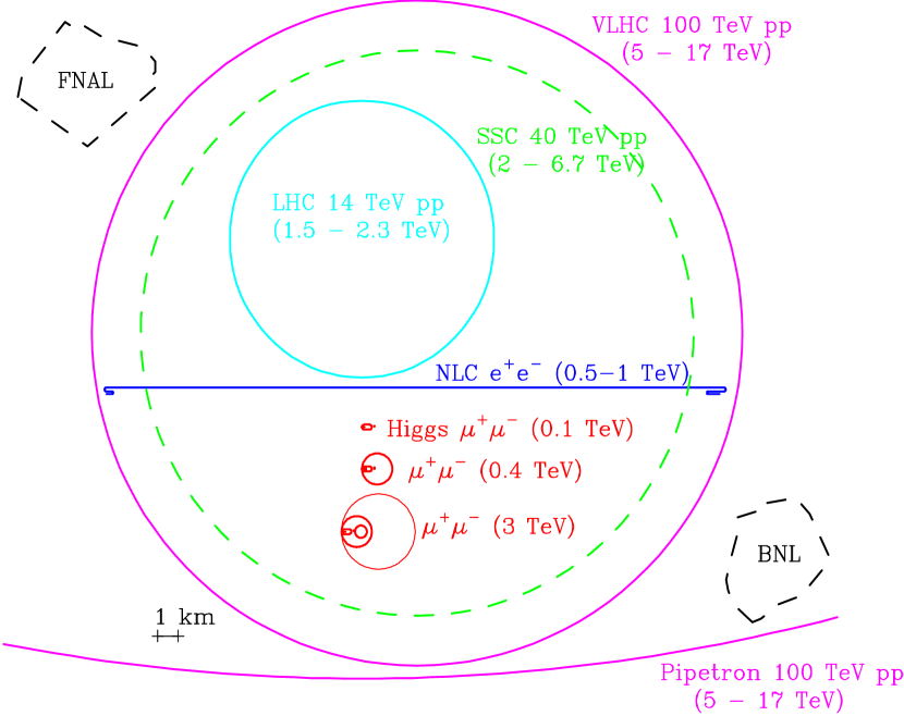
For a lepton with mass the radiative energy losses are inversely proportional to . Hence, the energy-loss problem can be solved by using heavy leptons. In practice this means using muons, which have a mass times that of an electron. The resulting reduction in radiative losses enables higher energies to be reached and smaller collider rings to be used [2, 3]. Parameters for 10 to 100 TeV collider have been discussed[4, 5]. Estimated sizes of the accelerator complexes required for 0.1-TeV, 0.5-TeV and 4-TeV muon colliders are compared with the sizes of other possible future colliders, and with the FNAL and BNL sites in Fig. 1. Note that muon colliders with CoM energies up to TeV would fit on these existing laboratory sites. The cost of building a muon collider is not yet known. However, since muon colliders are relatively small, they may be significantly less expensive than alternative machines.
Since muons decay quickly, large numbers of them must be produced to operate a muon collider at high luminosity. Collection of muons from the decay of pions produced in proton-nucleus interactions results in a large initial phase volume for the muons, which must be reduced (cooled) by a factor of for a practical collider. This may be compared with the antiproton stochastic cooling achieved in the Tevatron. In this case the 6-dimensional (6-D) phase space is reduced by approximately a factor of while with stacking the phase space density [6, 7] is increased by a factor of The technique of ionization cooling is proposed for the collider [8, 9, 10, 11]. This technique is uniquely applicable to muons because of their minimal interaction with matter.
Muon colliders also offer some significant physics advantages. The small radiative losses permit very small beam-energy spreads to be achieved. For example, momentum spreads as low as are believed to be possible for a low-energy collider. By measuring the time-dependent decay asymmetry resulting from the naturally polarized muons, it has been shown [12] that the beam energy could be determined with a precision of . The small beam-energy spread, together with the precise energy determination, would facilitate measurements of the masses and widths of any new resonant states scanned by the collider. In addition, since the cross-section for producing a Higgs-like scalar particle in the s-channel (direct lepton-antilepton annihilation) is proportional to , this extremely important process could be studied only at a muon collider and not at an collider [13]. Finally, the decaying muons will produce copious quantities of neutrinos. Even short straight sections in a muon-collider ring will result in neutrino beams several orders of magnitude higher in intensity than presently available, permitting greatly extended studies of neutrino oscillations, nucleon structure functions, the CKM matrix, and precise indirect measurements of the -boson mass[14] (see section II.I).
The concept of muon colliders was introduced by G. I. Budker [2, 3], and developed further by A. N. Skrinsky et al.[15, 16, 17, 18, 19, 20, 21, 22] and D. Neuffer [13, 23, 24, 25]. They pointed out the significant challenges in designing an accelerator complex that can make, accelerate, and collide and bunches all within the muon lifetime of s ( m). A concerted study of a muon collider design has been underway in the U.S. since 1992 [26, 27, 28, 29, 30, 31, 32, 33, 34, 35, 36, 37, 38, 39, 40, 41, 42]. By the Sausalito workshop [30] in 1995 it was realized that with new ideas and modern technology, it may be feasible to make muon bunches containing a few times muons, compress their phase space and accelerate them up to the multi-TeV energy scale before more than about 3/4 of them have decayed. With careful design of the collider ring and shielding it appears possible to reduce to acceptable levels the backgrounds within the detector that arise from the very large flux of electrons produced in muon decays. These realizations led to an intense activity, which resulted in the muon-collider feasibility study report [43, 44] prepared for the 1996 DPF/DPB Summer Study on High-Energy Physics (the Snowmass’96 workshop). Since then, the physics prospects at a muon collider have been studied extensively [45, 46, 47], and the potential physics program at a muon collider facility has been explored in workshops [39] and conferences [40].
Encouraged by further progress in developing the muon-collider concept, together with the growing interest and involvement of the high-energy-physics community, the Muon Collider Collaboration became a formal entity in May of 1997. The collaboration is led by an executive board with members from Brookhaven National Laboratory (BNL), Fermi National Accelerator Laboratory (FNAL), Lawrence Berkeley National Laboratory (LBNL), Budker Institute for Nuclear Physics (BINP), University of California at Los Angeles (UCLA), University of Mississippi and Princeton University. The goal of the collaboration is to complete within a few years the R&D needed to determine whether a Muon Collider is technically feasible, and if it is, to design the First Muon Collider.
| CoM energy | TeV | 3 | 0.4 | 0.1 | ||
|---|---|---|---|---|---|---|
| energy | GeV | 16 | 16 | 16 | ||
| ’s/bunch | ||||||
| Bunches/fill | 4 | 4 | 2 | |||
| Rep. rate | Hz | 15 | 15 | 15 | ||
| power | MW | 4 | 4 | 4 | ||
| /bunch | ||||||
| power | MW | 28 | 4 | 1 | ||
| Wall power | MW | 204 | 120 | 81 | ||
| Collider circum. | m | 6000 | 1000 | 350 | ||
| Ave bending field | T | 5.2 | 4.7 | 3 | ||
| Rms | % | 0.16 | 0.14 | 0.12 | 0.01 | 0.003 |
| 6-D | ||||||
| Rms | mm-mrad | 50 | 50 | 85 | 195 | 290 |
| cm | 0.3 | 2.6 | 4.1 | 9.4 | 14.1 | |
| cm | 0.3 | 2.6 | 4.1 | 9.4 | 14.1 | |
| spot | m | 3.2 | 26 | 86 | 196 | 294 |
| IP | mrad | 1.1 | 1.0 | 2.1 | 2.1 | 2.1 |
| Tune shift | 0.044 | 0.044 | 0.051 | 0.022 | 0.015 | |
| (effective) | 785 | 700 | 450 | 450 | 450 | |
| Luminosity | cm-2s-1 | |||||
| Higgs/year | ||||||
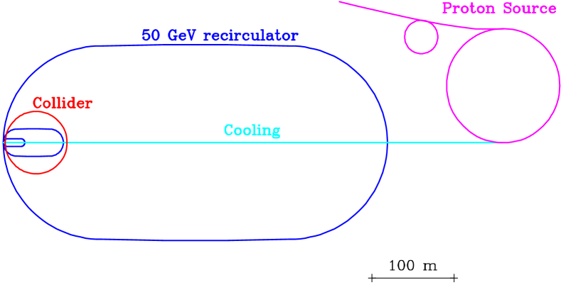
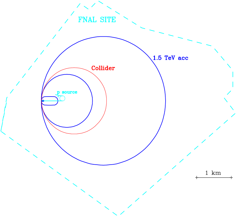
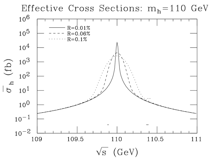
Table I gives the parameters of the muon colliders under study [48, 49, 50, 51, 52, 53, 54, 55], which have CoM energies of 0.1 TeV, 0.4 TeV and 3 TeV and Figs. 2 and 3 show possible outlines of the 0.1 TeV and 3 TeV machines. In the former case, parameters are given in the table for operation with three different beam-energy spreads: , 0.01, and 0.003%. In all cases, proton bunches containing 2.5- particles are accelerated to energies of 16 GeV. The protons interact in a target to produce charged pions of each sign. A large fraction of these pions can be captured in a high-field solenoid. Muons are produced by allowing the pions to decay into a lower-field solenoidal channel. To collect as many particles as possible within a useful energy interval, rf cavities are used to accelerate the lower-energy particles and decelerate the higher-energy particles (so-called phase rotation). With two proton bunches every accelerator cycle, the first used to make and collect positive muons and the second to make and collect negative muons, there are about muons of each charge available at the end of the decay channel per accelerator cycle. If the proton accelerator is cycling at 15 Hz, then in an operational year ( s), about positive and negative muons would be produced and collected.
As stated before, the muons exiting the decay channel populate a very diffuse phase space. The next step in the muon-collider complex is to cool the muon bunch, i.e., to turn the diffuse muon cloud into a very bright bunch with small longitudinal and transverse dimensions, suitable for accelerating and injecting into a collider. The cooling must be done within a time that is short compared to the muon lifetime. Conventional cooling techniques (stochastic cooling [56] and electron cooling [16]) take too long. The technique proposed for cooling muons is called ionization cooling [8, 10, 11], and will be discussed in detail in sec. V. Briefly, the muons traverse some material in which they lose both longitudinal and transverse momentum by ionization losses (). The longitudinal momentum is then replaced using an rf accelerating cavity, and the process is repeated many times until there is a large reduction in the transverse phase space occupied by the muons. The energy spread within the muon beam can also be reduced by using a wedge-shaped absorber in a region of dispersion (where the transverse position is momentum dependent). The wedge is arranged so that the higher-energy particles pass through more material than lower-energy particles. Initial calculations suggest that the 6-D phase space occupied by the initial muon bunches can be reduced by a factor of - before multiple Coulomb scattering and energy straggling limit further reduction. We reiterate that ionization cooling is uniquely suited to muons because of the absence of strong nuclear interactions and electromagnetic shower production for these particles at energies around 200 MeV/
Rapid acceleration to the collider beam energy is needed to avoid excessive particle loss from decay. It can be achieved, initially in a linear accelerator, and later in recirculating linear accelerators, rapid-cycling synchrotron, or fixed-field-alternating-gradient (FFAG) accelerators. Positive and negative muon bunches are then injected in opposite directions into a collider storage ring and brought into collision at the interaction point. The bunches circulate and collide for many revolutions before decay has depleted the beam intensities to an uninteresting level. Useful luminosity can be delivered for about 800 revolutions for the high-energy collider and 450 revolutions for the low-energy one.
There are many interesting and challenging problems that need to be resolved before the feasibility of building a muon collider can be demonstrated. For example, (i) heating from the very intense proton bunches may require the use of of a liquid-jet target, and (ii) attaining the desired cooling factor in the ionization-cooling channel may require the development of rf cavities with thin beryllium windows operating at liquid-nitrogen temperatures in high solenoidal fields. In addition, the development of long liquid-lithium lenses may be desirable to provide stronger radial focusing for the final cooling stages.
This article describes the status of our muon-collider feasibility studies, and is organized as follows. Section II gives a brief summary of the physics potential of muon colliders, including physics at the accelerator complex required for a muon collider. Section III describes the proton-driver specifications for a muon collider, and two site-dependent examples that have been studied in some detail. Section IV presents pion production, capture, and the pion-decay channel, and section V discusses the design of the ionization-cooling channel needed to produce an intense muon beam suitable for acceleration and injection into the final collider. Sections VI and VII describe the acceleration scenario and collider ring, respectively. Section VIII discusses backgrounds at the collider interaction point and section IX deals with possible detector scenarios. A summary of the conclusions is given in section X.
II THE PHYSICS POTENTIAL OF MUON COLLIDERS
A Brief overview
The physics agenda at a muon collider falls into three categories: First Muon Collider (FMC) physics at a machine with center-of-mass energies of 100 to 500 GeV; Next Muon Collider (NMC) physics at 3–4 TeV center-of-mass energies; and front-end physics with a high-intensity muon source.
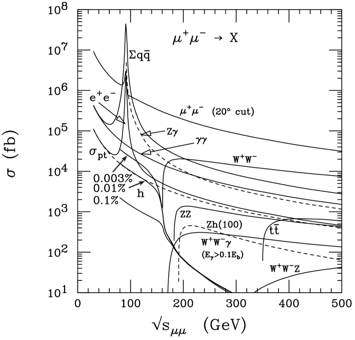
The FMC will be a unique facility for neutral Higgs boson (or techni-resonance) studies through -channel resonance production. Measurements can also be made of the threshold cross sections for production of , , , and pairs of supersymmetry particles — , , and — that will determine the corresponding masses to high precision. A factory, utilizing the partial polarization of the muons, could allow significant improvements in precision and in -mixing and CP-violating studies. In Fig. 4, we show the cross sections for SM processes versus the CoM energy at the FMC. For the unique -channel Higgs boson production, where , results for three different beam energy resolutions are presented.
The NMC will be particularly valuable for reconstructing supersymmetric particles of high mass from their complex cascade decay chains. Also, any resonances within the kinematic reach of the machine would give enormous event rates. The effects of virtual states would be detectable to high mass. If no Higgs bosons exist below 1 TeV, then the NMC would be the ideal machine for the study of strong scattering at TeV energies.
At the front end, a high-intensity muon source will permit searches for rare muon processes sensitive to branching ratios that are orders of magnitude below present upper limits. Also, a high-energy muon-proton collider can be constructed to probe high phenomena beyond the reach of the HERA collider. In addition, the decaying muons will provide high-intensity neutrino beams for precision neutrino cross-section measurements and for long-baseline experiments [57, 58, 59, 60, 61, 62, 63, 64, 65, 66]. Plus, there are numerous other new physics possibilities for muon facilities [44, 39] that we will not discuss in detail in this document.
B Higgs boson physics
The expectation that there will be a light (mass below ) SM-like Higgs boson provides a major motivation for the FMC, since such a Higgs boson can be produced with a very high rate directly in the -channel. Theoretically, the lightest Higgs boson of the most general supersymmetric model is predicted to have mass below GeV and to be very SM-like in the usual decoupling limit. Indeed, in the minimal supersymmetric model, which contains the five Higgs bosons , one finds GeV and the is SM-like if GeV. The light SUSY is regarded as the jewel in the SUSY crown. Experimentally, global analyses of precision electroweak data now indicate a strong preference for a light SM-like Higgs boson; this could well be the smoking gun for the SUSY Higgs boson. The goals of the FMC for studying the SUSY Higgs sector via -channel resonance production are: to measure the light Higgs mass, width, and branching fractions with high precision, in particular sufficient to differentiate the MSSM from the SM ; and, to find and study the heavier neutral Higgs bosons and .
The production of Higgs bosons in the -channel with interesting rates is a unique feature of a muon collider [45, 67]. The resonance cross section is
| (1) |
Gaussian beams with root-mean-square (rms) energy resolution down to are realizable. The corresponding rms spread in CoM energy is
| (2) |
The effective -channel Higgs cross section convolved with a Gaussian spread,
| (3) |
is illustrated in Fig. 5 for GeV, MeV, and resolutions , 0.06% and 0.1%. A resolution is needed to be sensitive to the Higgs width. The light Higgs width is predicted to be
| (4) |
for GeV, where the smaller values apply in the decoupling limit of large . We note that, in the MSSM, is required to be in the decoupling regime in the context of mSUGRA boundary conditions in order that correct electroweak symmetry breaking arises after evolution of parameters from the unification scale. In particular, decoupling applies in mSUGRA at , corresponding to the infrared fixed point of the top quark Yukawa coupling.
At , the effective -channel Higgs cross section is
| (5) |
BF denotes the branching fraction for decay; also, note that for . At GeV, the rates are
| (6) | |||||
| (7) |
assuming a -tagging efficiency . The effective on-resonance cross sections for other values and other channels () are shown in Fig. 6 for the SM Higgs. The rates for the MSSM Higgs are nearly the same as the SM rates in the decoupling regime of large .

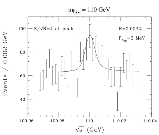
The important factors that make -channel Higgs physics studies possible at a muon collider are energy resolutions of order a few MeV, little bremsstrahlung and no beamstrahlung smearing, and precise tuning of the beam energy to an accuracy through continuous spin-rotation measurements [12]. As a case study, we consider a SM-like Higgs boson with GeV. Prior Higgs discovery is assumed at the Tevatron (in production with decay) or at the LHC (in production with decays with a mass measurement of MeV for an integrated luminosity of ) or possibly at a NLC (in giving MeV for ). A muon collider ring design would be optimized to run at energy . For an initial Higgs-mass uncertainty of MeV, the maximum number of scan points required to locate the -channel resonance peak at the muon collider is
| (8) |
for a resolution of MeV. The necessary luminosity per scan point () to observe or eliminate the -resonance at a significance level of is . (The scan luminosity requirements increase for closer to ; at the needed is a factor of 50 higher.) The total luminosity then needed to tune to a Higgs boson with GeV is . If the machine delivers (0.15 fb-1/year), then one year of running would suffice to complete the scan and measure the Higgs mass to an accuracy MeV. Figure 7 illustrates a simulation of such a scan.
Once the -mass is determined to MeV, a 3-point fine scan [45] can be made across the peak with higher luminosity, distributed with at the observed peak position in and at the wings (). Then, with the following accuracies would be achievable: 16% for , 1% for and 5% for . The ratio is sensitive to for values below 500 GeV. For example, for GeV [45]. Thus, using -channel measurements of the , it may be possible not only to distinguish the from the SM but also to infer .
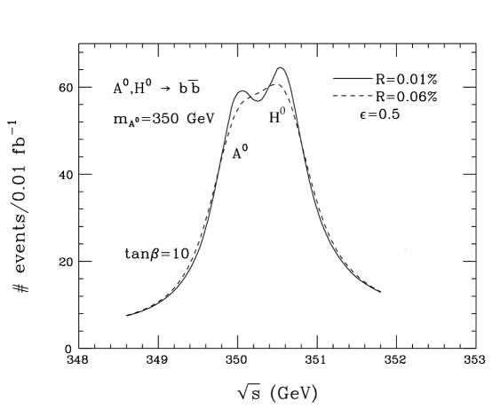
The study of the other neutral MSSM Higgs bosons at a muon collider via the -channel is also of major interest. Finding the and may not be easy at other colliders. At the LHC the region GeV is deemed to be inaccessible for –10 [68]. At an NLC the production process may be kinematically inaccessible if and are heavy (mass GeV for GeV). At a collider, very high luminosity () would be needed for studies.
At a muon collider the resolution requirements for -channel and studies are not as demanding as for the because the widths are broader; typically MeV for and GeV for . Consequently ( MeV) is adequate for a scan. This is important, since higher instantaneous luminosities (corresponding to ) are possible for (as contrasted with the for the much smaller preferred for studies of the ). A luminosity per scan point probes the parameter space with . The -range over which the scan should be made depends on other information available to indicate the and mass range of interest. A wide scan would not be necessary if is measured with the above-described precision to obtain an approximate value of .
In the MSSM, at large (as expected for mSUGRA boundary conditions), with a very close degeneracy in these masses for large . In such a circumstance, only an -channel scan with the good resolution possible at a muon collider may allow separation of the and states; see Fig. 8.
C Light particles in technicolor models
In most technicolor models, there will be light neutral and colorless technipion resonances, and , with masses below 500 GeV. Sample models include the recent top-assisted technicolor models [69], in which the technipion masses are typically above 100 GeV, and models [70] in which the masses of the neutral colorless resonances come primarily from the one-loop effective potential and the lightest state typically has mass as low as 10 to 100 GeV. The widths of these light neutral and colorless states in the top-assisted models will be of order 0.1 to 50 GeV [71]. In the one-loop models, the width of the lightest technipion is typically in the range from 3 to 50 MeV. Neutral technirho and techniomega resonances are also a typical feature of technicolor models. In all models, these resonances are predicted to have substantial Yukawa-like couplings to muons and would be produced in the -channel at a muon collider,
| (9) |
with high event rates. The peak cross sections for these processes are estimated to be – fb [71]. The dominant decay modes depend on eigenstate composition and other details but typically are [71]
| (10) | |||||
| (11) | |||||
| (12) | |||||
| (13) |
Such resonances would be easy to find and study at a muon collider.
D Exotic narrow resonance possibilities
There are important types of exotic physics that would be best probed in -channel production of a narrow resonance at a muon collider. Many extended Higgs sector models contain a doubly-charged Higgs boson (and its partner) that couples to via a Majorana coupling. The -channel process has been shown [72] to probe extremely small values of this Majorana coupling, in particular values naturally expected in models where such couplings are responsible for neutrino mass generation. In supersymmetry, it is possible that there is R-parity violation. If R-parity violation is of the purely leptonic type, the coupling for is very possibly the largest such coupling and could be related to neutrino mass generation. This coupling can be probed down to quite small values via -channel production at the muon collider [73].
E -factory
A muon collider operating at the -boson resonance energy is an interesting option for measurement of polarization asymmetries, – mixing, and of CP violation in the -meson system [74]. The muon collider advantages are the partial muon beam polarization, and the long -decay length for -mesons produced at this . The left-right asymmetry is the most accurate measure of , since the uncertainty is statistics dominated. The present LEP and SLD polarization measurements show standard deviations of 2.4 in , 1.9 in and 1.7 in [75]. The CP angle could be measured from decays. To achieve significant improvements over existing measurements and those at future -facilities, a data sample of -boson events/year would be needed. This corresponds to a luminosity /year, which is well within the domain of muon collider expectations; would be more than adequate, given the substantial GeV width of the .
F Threshold measurements at a muon collider
With 10 fb-1 integrated luminosity devoted to a measurement of a threshold cross-section, the following precisions on particle masses may be achievable [76]:
| (14) |
(if Precision and measurements allow important tests of electroweak radiative corrections through the relation
| (15) |
where represents loop corrections. In the SM, depends on and . The optimal precision for tests of this relation is , so the uncertainty on is the most critical. With MeV the SM Higgs mass could be inferred to an accuracy
| (16) |
Alternatively, once is known from direct measurements, SUSY loop contributions can be tested.
In top-quark production at a muon collider above the threshold region, modest muon polarization would allow sensitive tests of anomalous top quark couplings [77].
One of the important physics opportunities for the First Muon Collider is the production of the lighter chargino, [78]. Fine-tuning arguments in mSUGRA suggest that it should be lighter than 200 GeV. A search at the upgraded Tevatron for the process with and decays can potentially reach masses GeV with 2 fb-1 luminosity and GeV with 10 fb-1 [79]. The mass difference can be determined from the mass distribution.
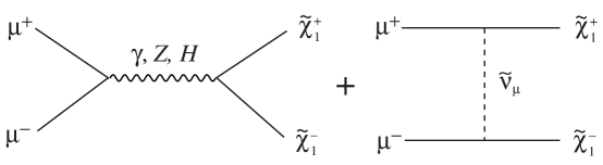
The two contributing diagrams in the chargino pair production process are shown in Fig. 9; the two amplitudes interfere destructively. The and masses can be inferred from the shape of the cross section in the threshold region [80]. The chargino decay is . Selective cuts suppress the background from production and leave signal efficiency for 4 jets events. Measurements at two energies in the threshold region with total luminosity and resolution can give the accuracies listed in table II on the chargino mass for the specified values of and .
| (MeV) | (GeV) | (GeV) |
|---|---|---|
| 35 | 100 | 500 |
| 45 | 100 | 300 |
| 150 | 200 | 500 |
| 300 | 200 | 300 |
G Heavy particles of supersymmetry
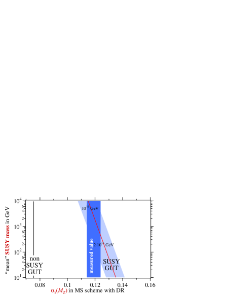
The requirements of gauge coupling unification can be used to predict the mean SUSY mass scale, given the value of the strong coupling constant at the -mass scale. Figure 10 shows the SUSY GUT predictions versus . For the value from a new global fit to precision electroweak data [75], a mean SUSY mass of order 1 TeV is expected. Thus, it is likely that some SUSY particles will have masses at the TeV scale. Large masses for the squarks of the first family are perhaps the most likely in that this would provide a simple cure for possible flavor changing neutral current difficulties.
At the LHC, mainly squarks and gluinos will be produced; these decay to lighter SUSY particles. The LHC will be a great SUSY machine, but some sparticle measurements will be very difficult or impossible there [81, 82], namely: (i) the determination of the LSP mass (LHC measurements give SUSY mass differences); (ii) study of sleptons of mass GeV because Drell-Yan production becomes too small at these masses; (iii) study of heavy gauginos and , which are mainly Higgsino and have small direct production rates and small branching fractions to channels usable for detection; (iv) study of heavy Higgs bosons when the MSSM parameter is not large and their masses are larger than , so that cross sections are small and decays to are likely to be dominant (their detection is deemed impossible if SUSY decays dominate).
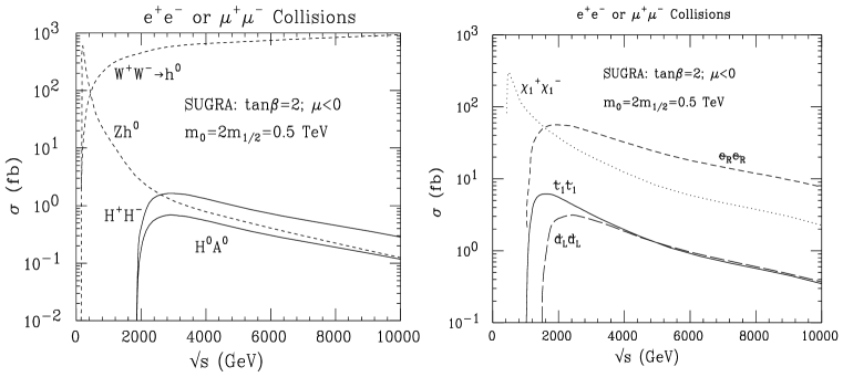
Detection and study of the many scalar particles predicted in supersymmetric models could be a particularly valuable contribution of a high energy lepton collider. However, since pair production of scalar particles at a lepton collider is -wave suppressed, energies well above threshold are needed for sufficient production rates; see Fig. 11. For scalar particle masses of order 1 TeV a collider energy of 3 to 4 TeV is needed to get past the threshold suppression. A muon collider operating in this energy range with high luminosity ( to ) would provide sufficient event rates to reconstruct heavy sparticles from their complex cascade decay chains [82, 84].
In string models, it is very natural to have extra bosons in addition to low-energy supersymmetry. The -channel production of a boson at the resonance energy would give enormous event rates at the NMC. Moreover, the -channel contributions of bosons with mass far above the kinematic reach of the collider could be revealed as contact interactions [85].
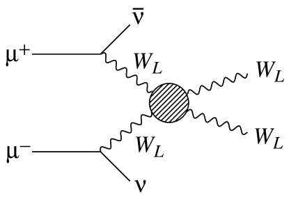
H Strong scattering of weak bosons
The scattering of weak bosons can be studied at a high-energy muon collider through the process in Fig. 12. The amplitude for the scattering of longitudinally polarized -bosons behaves like
| (17) |
if there is a light Higgs boson, and like
| (18) |
if no light Higgs boson exists; here is the square of the CoM energy and GeV. In the latter scenario, partial-wave unitarity of requires that the scattering of weak bosons becomes strong at energy scales of order 1 to 2 TeV. Thus, subprocess energies TeV are needed to probe strong scattering effects.
The nature of the dynamics in the sector is unknown. Models for this scattering assume heavy resonant particles (isospin scalar and vector) or a non-resonant amplitude based on a unitarized extrapolation of the low-energy theorem behavior . In all models, impressive signals of strong scattering are obtained at the NMC, with cross sections typically of order 50 fb-1 [86]. Event rates are such that the various weak-isospin channels () could be studied in detail as a function of . After several years of operation, it would even be possible to perform such a study after projecting out the different final polarization states (, and ), thereby enabling one to verify that it is the channel in which the strong scattering is taking place.
I Front end physics
New physics is likely to have important lepton flavor dependence and may be most apparent for heavier flavors. The intense muon source available at the front end of the muon collider will provide many opportunities for uncovering such physics.
1 Rare muon decays
The planned muon flux of muons/sec for a muon collider dramatically eclipses the flux, muons/sec, of present sources. With an intense source, the rare muon processes (for which the current branching fraction limit is ), conversion, and the muon electric dipole moment can be probed at very interesting levels. A generic prediction of supersymmetric grand unified theories is that these lepton flavor violating or CP-violating processes should occur via loops at significant rates, e.g. BF. Lepton-flavor violation can also occur via bosons, leptoquarks, and heavy neutrinos [87].
2 Neutrino flux
The decay of a muon beam leads to neutrino beams of well defined flavors. A muon collider would yield a neutrino flux 1000 times that presently available [88]. This would result in and events per year, which could be used to measure charm production (6% of the total cross section) and measure (and infer the -mass to an accuracy –50 MeV in one year) [57, 58, 59, 60, 61, 62, 63, 64, 65].
3 Neutrino oscillations
A special purpose muon ring has been proposed [58] to store or per year and obtain neutrinos per year from muon decays along 75-m straight sections of the ring, which would be pointed towards a distant neutrino detector. The neutrino fluxes from or from decays can be calculated with little systematic error. Then, for example, from the decays of stored ’s, the following neutrino oscillation channels could be studied by detection of the charged leptons from the interactions of neutrinos in the detector:
The detected or have the “wrong sign” from the leptons produced by the interactions of the and flux. The known neutrino fluxes from muon decays could be used for long-baseline oscillation experiments at any detector on Earth. The probabilities for vacuum oscillations between two neutrino flavors are given by
| (19) |
with in eV2 and in km/GeV. In a very long baseline experiment from Fermilab to the Gran Sasso laboratory or the Kamioka mine ( km) with -energies to 50 GeV (–200 km/GeV), neutrino charged-current interaction rates of /year would result. In a long baseline experiment from Fermilab to the Soudan mine (L=732 km), the corresponding interaction rate is /year. Such an experiment would have sensitivity to oscillations down to for [58].
4 collider
The possibility of colliding 200-GeV muons with 1000-GeV protons at Fermilab is under study. This collider would reach a maximum GeV2, which is 90 times the reach of the HERA collider, and deliver a luminosity , which is 300 times the HERA luminosity. The collider would produce neutral-current deep-inelastic-scattering events per year at , which is more than a factor of higher than at HERA. In the new physics realm, leptoquark couplings and contact interactions, if present, are likely to be larger for muons than for electrons. This collider would have sufficient sensitivity to probe leptoquarks up to a mass GeV and contact interactions to a scale –9 TeV [89].
J Summary of the physics potential
The First Muon Collider offers unique probes of supersymmetry (particularly -channel Higgs boson resonances) and technicolor models (via -channel production of techni-resonances), high-precision threshold measurements of and SUSY particle masses, tests of SUSY radiative corrections that indirectly probe the existence of high-mass squarks, and a possible factory for improved precision in polarization measurements and for -physics studies of CP violation and mixing.
The Next Muon Collider guarantees access to heavy SUSY scalar particles and states or to strong scattering if there are no Higgs bosons and no supersymmetry.
The Front End of a muon collider offers dramatic improvements in sensitivity for flavor-violating transitions (e.g., ), access to high- phenomena in deep-inelastic muon-proton and neutrino-proton interactions, and the ability to probe very small via neutrino-oscillation studies in long-baseline experiments.
The muon collider would be crucial to unraveling the flavor dependence of any type of new physics that is found at the next generation of colliders.
Thus, muon colliders are robust options for probing new physics that may not be accessible at other colliders.
III PROTON DRIVER
The overview of the required parameters is followed by a description of designs that have been studied in some detail. The section concludes with a discussion of the outstanding open issues.
A Specifications
The proton driver requirements are determined by the design luminosity of the collider, and the efficiencies of muon collection, cooling, transport and acceleration. The baseline specification is for a 4-MW, 16-GeV or a 7-MW, 30-GeV proton driver, with a repetition rate of 15 Hz and protons per cycle in 2 bunches (for the 100-GeV machine) or 4 bunches (for the higher energies) of or protons, respectively. Half the bunches are used to make and the rest for [90].
The total beam power is several MW, which is larger than that of existing synchrotrons. However, except for bunch length, these parameters are similar to those of Kaon factories [91] and spallation neutron sources [92]. As in those cases, the proton driver must have very low losses to permit inexpensive maintenance of components.
The rms bunch length for the protons on target has to be about 1 ns to: 1) reduce the initial longitudinal emittance of muons entering the cooling system, and 2) optimize the production of polarized muons. Although bunches of up to protons per cycle have been accelerated, the required peak current is 2000 A, which is unprecedented.
Since the collection of highly polarized ’s is inefficient (see section IV.G), the proton driver should eventually provide an additional factor of two or more in proton intensity to permit the luminosity to be maintained for polarized muon beams.
B Possible options
Accelerator designs are site, and to some extent, time dependent, and there have been three studies at three different energies (30 GeV [93], 16 GeV [94] and 24 GeV [95, 96, 97, 98]; see also [99]). In general, if the final energy is higher, the required currents are lower, bunch manipulation and apertures are easier, and the final momentum spread and space-charge tune shifts are less. Lowering the final energy gives somewhat more ’s/Watt, a lower rf requirement () and perhaps a lower facility cost.
In the low-energy muon collider, where two bunches of protons of are required on target, two bunches can be merged outside the driver. These two bunches would be extracted simultaneously from two different extraction ports, and fed by different transmission lines to the same target. By arranging the path lengths of the two lines appropriately, the two bunches can be exactly merged.
1 A generic design
A 7-MW collider-driver design based on parameters originally proposed in the Snowmass Feasibility study [93] consists of a 600-MeV linac, a 3.6-GeV booster and a 30-GeV driver. Both linac and booster are based on the BNL Spallation Neutron Source design [92], using a lower repetition rate and a lower total number of protons per pulse. For the 4-bunch case ( protons per bunch), the (95%) bunch area is assumed to be 2 eV-s at injection and eV-s at extraction. The driver lattice is derived from the lattice of the JHF driver using 90∘ FODO cells with missing dipoles in every third FODO cell, allowing a transition energy that is higher than the maximum energy or, perhaps, imaginary.
2 FNAL study
If a muon collider is built at an existing laboratory, then possibilities abound for symbiotic relationships with the other facilities and programs of that laboratory. For example, the proton driver for a muon collider might result from an upgrade of existing proton-source capabilities, and such an upgrade could then also enhance other future programs that use the proton beams.
Fermilab has conceived such a proton-source development plan [100] with three major components: an upgraded linac and two rapid-cycling (15 Hz) synchrotrons: a prebooster and a new booster. The two synchrotrons operate in series; the four proton bunches for the muon collider are formed in the prebooster and then accelerated sequentially in the prebooster and the booster. The plan could be implemented in stages, and other programs would benefit from each stage, but all three components are required to meet the luminosity goals of the muon colliders that have been considered so far.
| Linac | Booster | Driver | |
|---|---|---|---|
| Energy range (GeV) | 1 | 3 | 16 |
| Rep. rate (Hz) | 15 | 15 | 15 |
| RF voltage per turn (MV) | 0.15 | 1.5 | |
| Circumference (m) | 158 | 474 | |
| Protons per bunch () | |||
| Beam emittance [95%] ( mm-mrad ) | 200 | 240 | |
| Bunch area [95%] (eV-s) | 1.5 | ||
| Incoherent tune shift @ Inj. | 0.39 | 0.39 |
Table III presents the major parameters of the two rings. Whenever the needs of the muon collider itself allow some flexibility, the parameters have been chosen to optimize the resulting facility as a proton source for the rest of the future program at Fermilab. For example, the machine circumferences and rf-harmonic numbers result in bunch trains that are compatible with the existing downstream proton machines.
A muon collider requires proton bunches that are both very intense and, at the pion-production target, very short. Strong transverse and longitudinal space-charge forces might disrupt such bunches in the synchrotrons unless measures to alleviate those effects are incorporated in the design. The Laslett incoherent-space-charge tune shift quantifies the severity of the transverse effects. A useful approximation for the space-charge tune shift at the center of a round Gaussian beam is
| (20) |
In this expression m is the so-called electromagnetic radius of the proton, is the total number of protons in the ring, is the 95% normalized transverse emittance, and are the usual Lorentz kinematical factors, and is the bunching factor, defined as the ratio of the average beam current to the peak current.
The approximation (20) implies that for a given total number of protons, here , the factors in the denominator are the only ways to reduce the tune shift to a specified maximum tolerable value, taken as 0.4. The bunching factor can be raised somewhat by careful tailoring of beam distributions, but here a typical value of 0.25 is conservatively assumed. Achieving the desired beam intensity then requires a combination of high injection energy, here taken as 1 GeV into the first ring, and large transverse normalized emittances, here assumed to be about mm-mrad. The corresponding required aperture is about 13 cm in the first ring and about 10 cm in the second ring. With such large apertures in rapid-cycling synchrotrons, careful design of the beam pipes for both rings is required to manage eddy-current effects. Two approaches are under consideration. One is a thin Inconel pipe with water cooling and eddy-current coil corrections integrated on the pipe, as in the AGS Booster. The other is a ceramic beam pipe with a conductor inside to carry beam-image currents, as in ISIS.
The Fermilab linac presently delivers a 400-MeV beam, and is capable with modest modifications of accelerating as many as protons per cycle at 15 Hz [101]. A significant upgrade is required in order to deliver protons at 1 GeV. The energy can be raised by appending additional side-coupled modules to the downstream end of the linac. Increasing the linac beam intensity probably means increasing both the beam current and the duration of the beam pulse. Injection into the first ring is by charge stripping of the beam; the incoming beam will be chopped and injected into pre-existing buckets to achieve high capture efficiency.
The circumference of the second ring is set equal to that of the existing Fermilab Booster. This choice provides several advantages. First, the new booster could occupy the same tunnel as a relocated Booster; secondly, the beam-batch length from a full second ring matches that of the present Booster, which simplifies matching to downstream machines for other programs. The output energy of 16 GeV then results from an assumed dipole packing fraction of 0.575 and a peak dipole field of 1.3 T, which is the highest dipole field that is consistent with straightforward, nonsaturating design of magnets having thin silicon-steel laminations. Driving such magnets into saturation would cause significant heating of the magnet yoke as well as potential problems with tracking between the dipoles and quadrupoles.
The prebooster also has 1.3-T dipole fields, and its circumference is one third that of the new booster; it operates at an rf harmonic number . The strategy for achieving the required short bunches at the target while alleviating space-charge effects in the rings is to start with four bunches occupying most of the circumference of the first small ring in order to keep the bunching factor large, and to do a bunch-shortening rotation in longitudinal phase space just before extraction from the second synchrotron. The four bunches are accelerated in the first ring to 3 GeV, then transferred bunch-to-bucket into the second ring with its harmonic number . At that energy, the kinematic factor in the tune-shift formula (20) is large enough to compensate for the smaller bunching factor in the second ring. The transfer energy of 3 GeV between the two rings roughly equalizes their space-charge tune shifts.
Both rings employ separated-function lattices with flexible momentum compaction in order to raise their transition energies above their respective extraction energies. This not only avoids having to accelerate beam through transition but also provides other advantages. Intense beams are not subject to certain instabilities such as the negative-mass instability below transition and empirically seem less susceptible to other instabilities such as the microwave instability. Also, the negative natural chromaticity is beneficial for stabilizing the beam below transition, thereby perhaps obviating the need for sextupole correctors, especially in the first ring. Having transition not too far above extraction also provides substantial bucket area in which to accomplish beam-shortening rf manipulations.
Several potential sources of instabilities in the rings have been examined [102], as well as the possibility of compensating the latter effect by inductive inserts in the rings. Space charge is the main factor affecting the stability of the beams; the rings appear to be safe from longitudinal- and transverse-microwave instabilities. Of course, standard stabilizing methods such as active dampers are necessary to counteract some of the instabilities. Flexible momentum-compaction lattices would be useful not only to raise the transition energy above the extraction energy, but also to allow fast changes in the slip factor to facilitate bunch-narrowing manipulations at extraction time. Compensation of longitudinal space-charge effects by means of ferrite-loaded inductive inserts would be useful, especially for the first ring.
The magnet-power-supply circuit for each ring is a 15-Hz resonant system like that of the existing Booster, with dipoles and quadrupoles electrically in series. This implies that the second ring will accelerate only one batch at a time from the first ring, which is all that the muon collider needs. Adding about 15% of second harmonic to the magnet ramp reduces the required peak accelerating voltage by about 25%, which is probably worth doing, especially for the second ring with its large voltage requirement.
One of the advantages of a two-ring system is that the two rings divide the work of accelerating the beam. The rf system of the first ring is relatively modest because of its small circumference and small energy gain; that of the second ring is simplified because its high injection energy means a small rf-frequency swing [103].
ESME simulations of longitudinal motion show that the rms bunch length is 2 nsec as desired after the bunch rotation that occurs just before extraction from the second synchrotron.The bunch rotation creates momentum spreads of about 2% with longitudinal emittances of about 2 eV-s per bunch. Such spreads would contribute a few cm in quadrature to the beam size for a short period before extraction. This is thought to be tolerable, given the large apertures that are required in any case. High injection energies help to alleviate these longitudinal effects, which result from space-charge voltages having the same kinematic dependence as the transverse tune shifts.
3 AGS upgrade
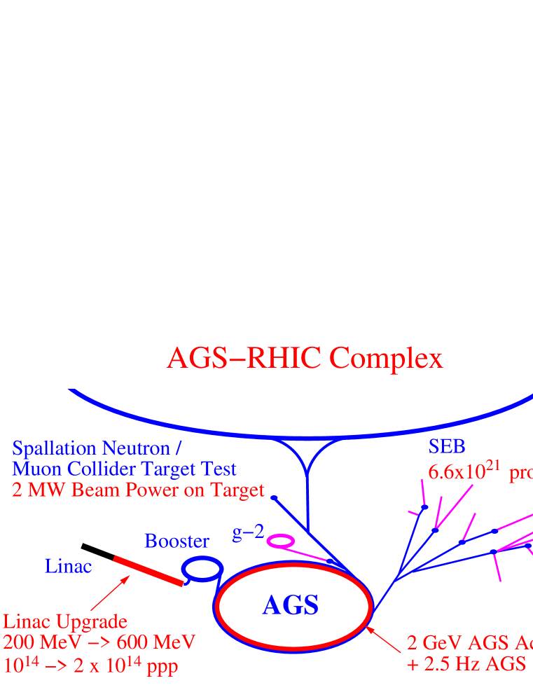
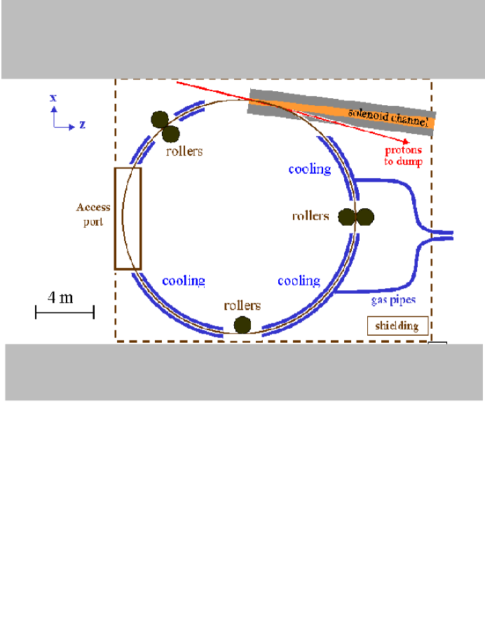
The third study [95, 96, 97, 98] is of an upgrade to the BNL AGS, which should produce bunches larger than those required for the muon collider, but at a lower repetition rate. The AGS presently produces protons in eight bunches at 25 GeV and 0.6 Hz. A 2.5-GeV accumulator ring in the AGS tunnel and AGS power-supply upgrade to 2.5-Hz operation would match the repetition rate to the 10-Hz repetition rate of the booster. This would generate 1 MW beam power. With an additional upgrade of the linac energy to 600 MeV, an intensity of protons per pulse in four bunches of at 25 GeV and 2.5 Hz could be reached, raising the power to 2 MW. The upgrades to the AGS accelerator complex are summarized in Fig.13. Other options are also under consideration, such as the addition of a second booster and 5-Hz operation, that would reach the baseline specification of 4 MW.
The AGS momentum acceptance of % requires that the longitudinal phase space occupied by one bunch be less than 4.5 eV-s. This high bunch density in turn generates stringent demands on the earlier parts of the accelerator cycle. In particular, Landau damping from the beam momentum spread may guard against resistive wall instabilities during injection and longitudinal microwave instabilities after transition. Beam stability can be restored with a more-powerful transverse-damping system and possibly a new low-impedance vacuum chamber. The transverse microwave instability is predicted to occur after transition crossing unless damped by Landau damping from incoherent tune spread or possibly high-frequency quadrupoles.
C Progress and open issues
Conventional rf manipulations appear able to produce 1- to 2-ns proton bunches if enough rf voltage to overcome the space-charge forces is used, and the beam energy is far enough from transition so the final bunch rotation is fast. Both simulations and experimental work have been directed at demonstrating that a short pulse can be produced easily.
An experiment at the AGS has shown that bunches with ns can be produced near transition from bunches with ns by bunch rotation [104, 105]. In this experiment, the AGS was flattoped near transition ( GeV) while the -jump system was used to bring the transition energy suddenly to the beam energy, letting the bunch-energy spread expand and bunch length contract. The experiment also demonstrated that bunches are stable over periods of 0.1 s. In addition, the data were used to measure the lowest two orders of the momentum compaction factor.
The AGS bunch area, 1.5 eV-s, was comparable to that expected in the proton driver, but the bunch charge (though as large as 3- protons) was only about one tenth of that required by the muon target. The proton driver would use a flexible momentum compaction lattice which would give much better control of the transition energy, permitting a very fast final bunch rotation [106]. In addition, the rf frequency would be higher than that of the AGS so the buckets (and bunches) would initially be only half as long. Thus bunch rotation could be expected to be easier with the new machine, which should compensate for the larger charge.
Simulations with the ESME code have also shown that 1-2 ns bunches of can be produced at extraction in a 16-GeV ring with the rf and emittance shown in Table III.
The efficiency of capturing and accelerating beam may be increased by compensation of the space-charge forces in the proton driver. The use of tunable inductive inserts in the ring vacuum chamber may permit active control and compensation of the longitudinal space charge below transition (since the inductive impedance is of the opposite sign to the capacitive space charge). Initial experiments at the KEK proton synchrotron and Los Alamos PSR [107] with short ferrite inserts appear to show a reduction in the synchrotron oscillation frequency shift caused by space charge and a decrease in the necessary rf voltage to maintain a given bunch intensity. Further experiments are needed to demonstrate this technique fully.
The high rf voltage and beam power and the relatively small size of the machine require high-gradient, high-power rf cavities. Fermilab, BNL and KEK are collaborating on research and development of such type of cavities.This work includes the study of magnet alloys and hybrid cavities using both ferrite and new magnet alloys, high-power amplifiers and beam-loading compensation.
The employment of barrier-bucket [108] rf cavities can effectively generate and manipulate a gap in the beam and reduce the space-charge effect. A successful test of this scheme has recently been completed [109], and two kV barrier cavities have been built by BNL and KEK and are being installed on the AGS. Another high-gradient barrier cavity using magnet alloys is under study at Fermilab.
IV PION PRODUCTION, CAPTURE AND PHASE ROTATION CHANNEL
This section first discusses the choice of target technology and optimization of the target geometry, and then describes design studies for the pion capture and phase rotation channel. Prospects for polarized muon beams are discussed in detail. The section concludes with an outline of an R&D program for target and phase rotation issues.
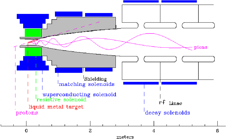
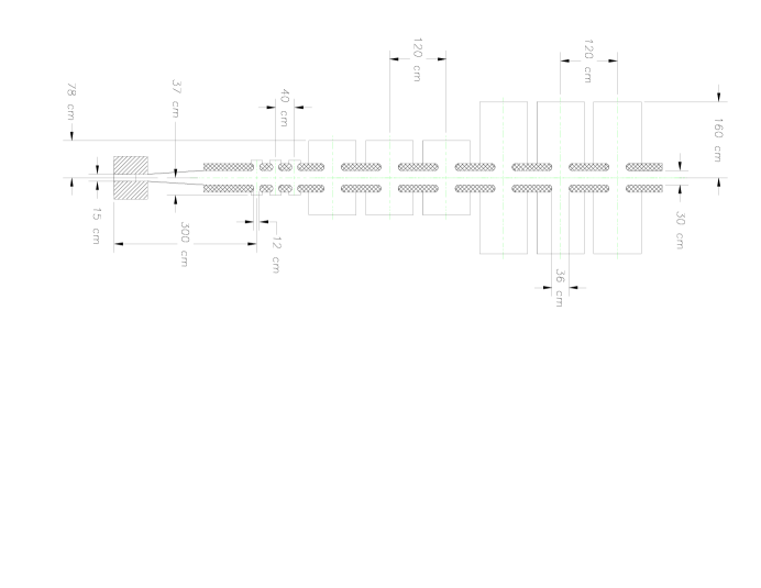
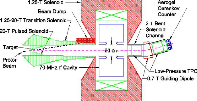
Figure 14 gives an overview of the configuration for production of pions by a proton beam impinging on a long, transversely thin target, followed by capture of low-momentum, forward pions in a channel of solenoid magnets with rf cavities to compress the bunch energy while letting the bunch length grow. This arrangement performs the desired rotation of the beam.
A Pion production
To achieve the luminosities for muon colliders presented in Table I, (or in the 100 GeV CoM case) muons of each sign must be delivered to the collider ring in each pulse. We estimate that a muon has a probability of only 1/4 of surviving the processes of cooling and acceleration, due to losses in beam apertures or by decay. Thus, muons (1.6 at 100 GeV) must exit the phase rotation channel each pulse. For pulses of protons ( for 100 GeV), this requires 0.3 muons per initial proton. Since the efficiency of the phase rotation channel is about 1/2, this is equivalent to a capture of about 0.6 pions per proton: a very high efficiency.
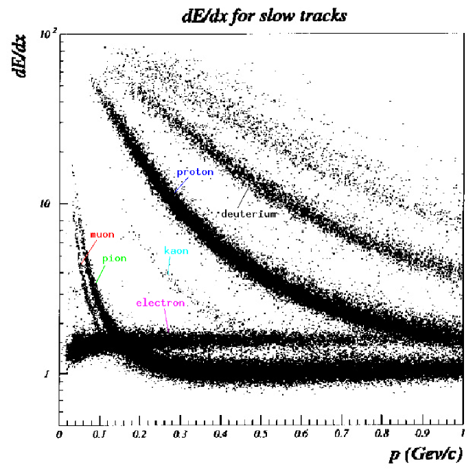
The pions are produced in the interaction of the proton beam with the primary target. Extensive simulations have been performed for pion production from 8-30 GeV proton beams on different target materials in a high-field solenoid [44, 110, 111, 112, 113]. Three different Monte Carlo codes [114, 115, 116, 117] predict similar pion yields despite significant differences in their physics models. Some members of the Collaboration are involved in an AGS experiment BNL E-910 [118] to measure the yield of very low momentum pions, which will validate the codes in the critical kinematic region. This experiment ran for 14 weeks during the Spring of 1996 and has collected over 20 million events, of which about a quarter are minimum bias triggers for inclusive cross section measurements. The targets were varied in material (Be, Cu, Au, U) and thickness (2–100% interaction length ()) and three different beam momenta were used (6, 12.5, 18 GeV/ Presently, the E910 collaboration is doing a careful analysis of the large data sample obtained. Figure 15 shows the dE/dx energy vs. momentum for reconstructed tracks in the TPC; there is clear particle species separation [119].
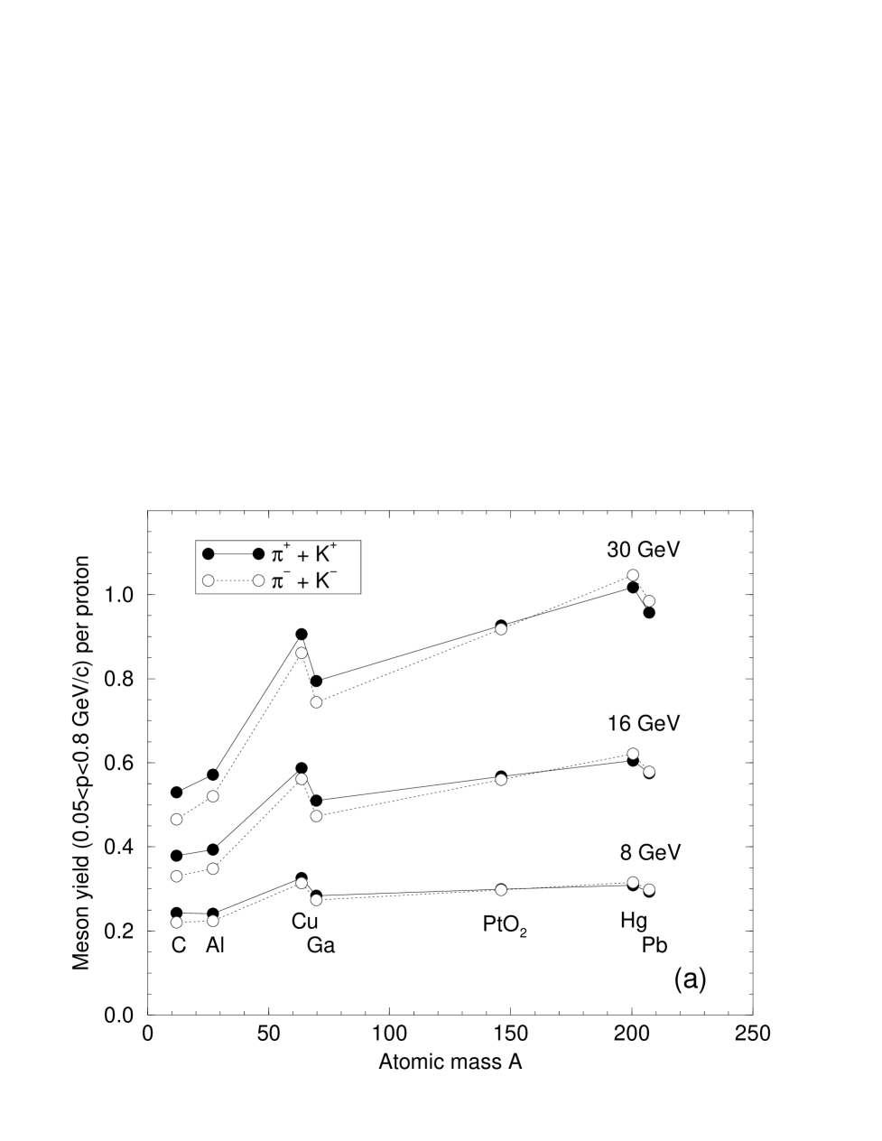
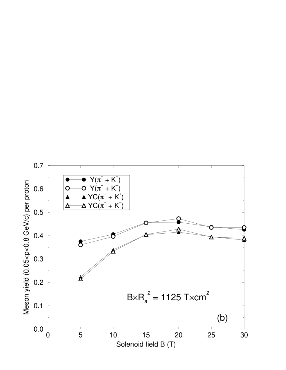
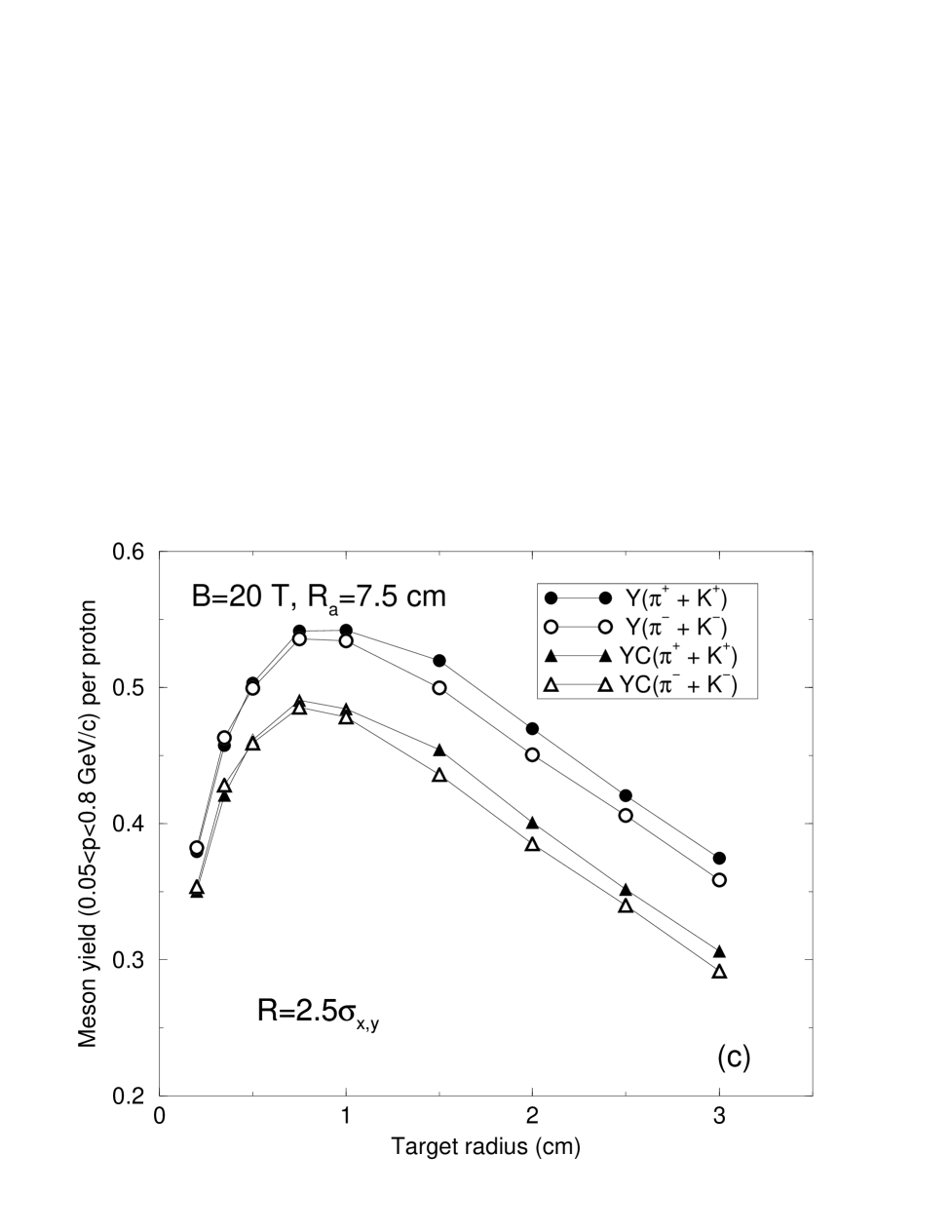
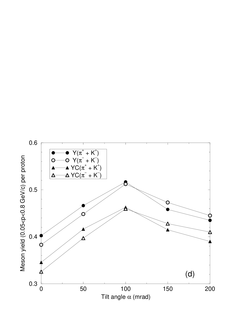
The pion yield is greater for relatively high materials, and for these, the pion yield is maximal for longitudinal momenta of the same order as the average transverse momentum ( MeV/). Targets of varying composition (), radii (0.2-3 cm) and thicknesses (0.5-3 nuclear interaction lengths) have been explored using a Monte Carlo simulation [111]. For a fixed number of interaction lengths, the pion yield per proton rises almost linearly with proton energy, and hence almost proportional to the energy deposited in the target. The yield is higher for medium- and high- target materials, with a noticeable gain at for 30 GeV proton beams, but with only a minor effect for GeV. This is shown in Fig. 16 where results of detailed MARS13(98) [115] simulations are presented. The curves show the meson yield () from the targets in the momentum interval GeV/ (labeled Y) and the number of mesons that are both captured in the high field solenoid and transported into the decay channel (labeled YC). The typical statistical error is a few percent.
B Target
The target should be 2-3 interaction lengths long to maximize pion production. A high-density material is favored to minimize the size and cost of the capture solenoid magnet. Target radii larger than about 1 cm lead to lower pion rates due to reabsorption, while smaller diameter targets have less production from secondary interactions. Tilting the target by 100-150 mrad minimizes loss of pions by absorption in the target after one turn on their helical trajectory [50, 120]. Another advantage of the tilted target geometry is that the high energy and neutral components of the shower can be absorbed in a water-cooled beam dump to the side of the focused beam.
About 30 kJ of energy is deposited in the target by each proton pulse (10% of the beam energy). Hence, the target absorbs 400 kW of power at the 15-Hz pulse rate. Cooling of the target via contact with a thermal bath would lead to unacceptable absorption of pions, and radiative cooling is inadequate for such high power in a compact target. Therefore, the target must move so as to carry the energy deposited by the proton beam to a heat exchanger outside the solenoid channel.
Both moving solid metal and flowing liquid targets have been considered, with the latter as the currently preferred solution. A liquid is relatively easy to move, easy to cool, can be readily removed and replaced, and is the preferred target material for most spallation neutron sources under study. A liquid flowing in a pipe was considered, but experience at ISOLDE with short proton pulses [121] as well as simulations [122, 123] suggest serious problems in shock damage to the pipe. An open liquid jet is thus proposed.
A jet of liquid mercury has been demonstrated [122] but not exposed to a beam. For our application, safety and other considerations favor the use of a low melting point lead alloy rather than mercury. Gallium alloys, though with lower density, are also being considered. Experimental and theoretical studies are underway to determine the consequences of beam shock heating of the liquid. It is expected that the jet will disperse after being exposed to the beam. The target station must survive damage resulting from the violence in this dispersion. This consideration will determine the minimum beam, and thus jet, radius.
For a conducting liquid jet in a strong magnetic field, as proposed, strong eddy currents will be induced in the jet, causing reaction forces that may disrupt its flow [124, 125]. The forces induced are proportional to the square of the jet radius, and set a maximum for this radius of order 5-10 mm. If this maximum is smaller than the minimum radius set by shock considerations, then multiple smaller beams and jets could be used; e.g., four jets of 5 mm radius with four beams with protons per bunch. Other alternatives include targets made from insulating materials such as liquid PtO2 or Re2O3, slurries (e.g., Pt in water), or powders [126].
A moving solid metal target is not the current baseline solution, but is a serious possibility. In this case, the target could consist of a long flat band or hoop of copper-nickel that moves along its length (as in a band saw) [127]. The band would be many meters in length, would be cooled by gas jets away from the target area, and would be supported and moved by rollers, as shown in Fig. 17.
The choice and parameters of the target are critical issues that need resolution. These can be resolved by experiments with a strong magnetic field and a beam, as discussed in section IV.H.
C Capture
To capture all pions with transverse momenta less than their typical value of 200 MeV/, the product of the capture solenoid field and its radius must be greater than 1.33 T m. The use of a high field and small radius is preferred to minimize the corresponding transverse emittance, which is proportional to : for a fixed transverse momentum capture, this emittance is thus proportional to . A field of 20 T and 7.5 cm radius was chosen on the basis of simulations described below. This gives = 1.5 T m, T m2 and a maximum transverse momentum capture of MeV/.
A preliminary design [128] of the capture solenoid has an inner 6 T, 4 MW, water cooled, hollow conductor magnet with an inside diameter of 24 cm and an outside diameter of 60 cm. There is space for a 4 cm thick, water cooled, heavy metal shield inside the coil. The outer superconducting magnet has three coils, with inside diameters of 60 to 80 cm. It generates an additional 14 T of field at the target and provides the required tapered field to match into the decay channel. Such a hybrid solenoid has parameters compatible with those of existing magnets [129].
The 20 T capture solenoid is matched via a transfer solenoid [110] into a decay channel consisting of a system of superconducting solenoids with the same adiabatic invariant . Thus, for a 1.25 T decay channel, drops by a factor of 16 between the target and decay channel, and change by factors of 4 and 1/4, respectively. This permits improved acceptance of transverse momentum within the decay channel, at the cost of an increased spread in longitudinal momentum. Figure 16(b) shows the meson yield as a function of field in the capture solenoid, with the radius of the capture solenoid adjusted to maintain the same as in the decay channel. The optimum field is 20 T in the capture solenoid.
If the axis of the target is coincident with that of the solenoid field, then there is a relatively high probability that pions re-enter the target after one cycle on their helical trajectory and are lost due to nuclear interactions. When the target and proton beam are set at an angle of 100-150 mrad with respect to the field axis [111], the probability for such pion interactions at the target is reduced, and the overall production rate is increased by 60%, as shown in Fig. 16(d).
In summary, the simulations indicate that a 20 T solenoid of 16 cm inside diameter surrounding a tilted target will capture about half of all produced pions. With target efficiency included, about 0.6 pions per proton will enter the pion decay channel [111].
D Phase rotation linac
The pions, and the muons into which they decay, have a momentum distribution with an rms spread of approximately 100% and a peak at about 200 MeV/. It would be difficult to handle such a wide spread in any subsequent system. A linac is thus introduced along the decay channel, with frequencies and phases chosen to decelerate the fast particles and accelerate the slow ones; i.e., to phase rotate the muon bunch. Several studies have been made of the design of this system, using differing ranges of rf frequency, delivering different final muon momenta, and differing final bunch lengths. In all cases, muon capture efficiencies of close to 0.3 muons per proton are obtained. Until the early stages of the ionization cooling have been designed, it is not yet possible to choose between them. Independent of the above choices is a question of the location of the focusing solenoid coils and rf cavity design, as discussed below in the section IV.F.
| Linac | Length | Frequency | Gradient |
| (m) | (MHz) | (MeV/m) | |
| 1 | 3 | 60 | 5 |
| 2 | 29 | 30 | 4 |
| 3 | 5 | 60 | 4 |
| 4 | 5 | 37 | 4 |
1 Lower energy, longer bunch example
This example captures muons at a mean kinetic energy of 130 MeV. Table IV gives parameters of the linacs used. Monte Carlo simulations [52], with the program MUONMC [130], were done using pion production calculated by ARC [114] for a copper target of 1-cm radius at an angle of 150 mrad. A uniform solenoidal field was assumed in the phase rotation, and the rf was approximated by a series of kicks.
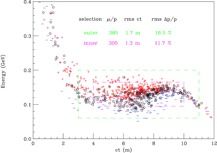
Figure 18 shows the energy vs. at the end of the decay and phase rotation channel. The abscissa is a measure of bunch length at the end of the channel: the total transit time of each is multiplied by the velocity of light and the total length of the channel is subtracted. Thus a ficticious reference particle at the center of the incident bunch at the target arrives at m. A loose final bunch selection was defined with an energy MeV and bunch from 3 to 11 m. With this selection, the rms energy spread is 16.5%, the rms is 1.7 m, and there are 0.39 muons per incident proton. A tighter selection with an energy MeV and bunch from 4 to 10 m gave an rms energy spread of 11.7%, rms of 1.3 m, and contained 0.31 muons per incident proton.
2 Higher energy, shorter bunch example
In this example the captured muons have a mean kinetic energy close to 320 MeV. It is based on a Monte Carlo study which uses the updated MARS pion production model [116] to generate pions created by 16 GeV protons on a 36 cm long, 1 cm radius coaxial gallium target. Figure 19 shows the longitudinal phase space of the muons at the end of an 80 m long, 5 T solenoidal decay channel with cavities of frequency in the 30-90 MHz range and acceleration gradients of 4-18 MeV/m. A total of 0.33 muons per proton fall within the indicated cut (6 m300 MeV). The rms bunch length inside the cut is 148 cm and rms energy spread is 62 MeV. The normalized six dimensional (6-D) emittance is 217 cm3 and the transverse part is 1.86 cm (the normalized 6-D emittance is defined in section V).
A sample simulation with lithium hydride absorbers regularly spaced in the last 60 m of a 120 m decay channel and with compensating acceleration captures 0.3 muons with mean kinetic energy of about 380 MeV in a (6 m300 MeV) window. The longitudinal phase space is about the same as in the previous example but the transverse part shrinks to 0.95 cm due to ionization cooling which reduces the 6-D phase space to 73.5 cm

E Use of both signs
Protons on the target produce pions of both signs, and a solenoid will capture both, but the subsequent rf systems will have opposite effects on each sign. The proposed baseline approach uses two separate proton bunches to create separate positive and negative pion bunches and accepts the loss of half the pions/muons during phase rotation.
If the pions can be charge separated with limited loss before the phase rotation cavities are reached, then higher luminosity may be obtained. The separation of charged pions in a curved solenoid decay line was studied in [110]. Because of the resulting dispersion in a bent solenoid, an initial beam of radius with maximum-to-minimum momentum ratio will require a large beampipe of radius downstream to accommodate the separated beams. A septum can then be used to capture the two beams into separate channels. Typically the reduction in yield for a curved solenoid compared to a straight solenoid is about 25% (due to the loss of very low and very high momentum pions to the walls or septum), but this must be weighed against the fact that both charge signs are captured for an overall net gain. A disadvantage is that this charge separation takes place over several meters of length during which time the beam spreads longitudinally. This makes capture in an rf phase rotation system difficult, although a large aperture cavity system could be incorporated in the bent solenoid region to alleviate this. The technique deserves further study and may be useful to consider as an intensity upgrade to a muon collection system.
F Solenoids and rf
As noted above, capture using higher frequencies appears to be less efficient, and most studies now use frequencies down to 30 MHz. Such cavities, when conventionally designed, are very large (about 6.6 m diameter). In the Snowmass study [131] a reentrant design reduced this diameter to 2.52 m, but this is still large, and it was first assumed that the 5 T focusing solenoids would, for economic reasons, be placed within the irises of the cavities (see Fig. 20).
A study of transmission down a realistic system of iris located coils revealed betatron resonant excitation from the magnetic field periodicities, leading to significant particle loss. This was reduced by the use of more complicated coil shapes [131], smaller gaps, and shorter cavities, but remained a problem.
An alternative is to place continuous focusing coils outside the cavities as shown in Fig. 14. In this case, cost will be minimized with lower magnetic fields (1.25-2.5 T) and correspondingly larger decay channel radii (21-30 cm). Studies are underway to determine the optimal solution.
G Polarization
Polarization of the muon beams presents a significant physics advantage over the unpolarized case, since signal and background of electroweak processes usually come predominantly from different polarization states.
1 Polarized muon production
In the center of mass of a decaying pion, the outgoing muon is fully polarized ( for and +1 for ). In the lab system the polarization depends on the decay angle and initial pion energy [132, 133, 134]. For pion kinetic energy larger than the pion mass, the average polarization is about 20%, and if nothing else is done, the polarization of the captured muons after the phase rotation system is approximately this value.
If higher polarization is required, some selection of muons from forward pion decays is required. Figure 18, above, showed the polarization of the phase rotated muons. The polarization {P, , and P} is marked by the symbols and respectively. If a selection is made on the minimum energy of the muons, then greater polarization is obtained. The tighter the cut, the higher the polarization, but the less the fraction of muons that survive. Figure 21 gives the results of a Monte Carlo study.
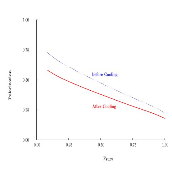
If this selection is made on both beams, and if the proton bunch intensity is maintained, then each muon bunch is reduced by the factor and the luminosity would fall by . But if, instead, proton bunches are merged so as to obtain half as many bunches with twice the intensity, then the muon bunch intensity is maintained and the luminosity (and repetition rate) falls only as .
The luminosity could be maintained at the full unpolarized value if the proton source intensity could be increased. Such an increase in proton source intensity in the unpolarized case might be impractical because of the resultant excessive high energy muon beam power, but this restriction does not apply if the increase is used to offset losses in generating polarization.
Thus, the goal of high muon beam polarization may shift the parameters of the muon collider towards lower repetition rate and higher peak currents in the proton driver.
2 Polarization preservation
The preservation of muon polarization has been discussed in some detail in [135]. During the ionization cooling process the muons lose energy in material and have a spin-flip probability
| (21) |
where is the fractional loss of energy due to ionization. In our case, the integrated energy loss is approximately 3 GeV and the typical energy is 150 MeV, so the integrated spin-flip probability is close to 10%. The change in polarization is twice the spin-flip probability, so the reduction in polarization is approximately 20%. This loss is included in Fig. 21.
During circulation in any ring, the muon spin, if initially longitudinal, will precess by turns per revolution, where is . A given energy spread will introduce variations in these precessions and cause dilution of the polarization. But if the particles remain in the ring for an exact integer number of synchrotron oscillations, then their individual average ’s will be the same and no dilution will occur.
In the collider, bending can be performed with the spin orientation in the vertical direction, and the spin rotated into the longitudinal direction only for the interaction region. The design of such spin rotators appears relatively straightforward, but long. This might be a preferred solution at high energies but is not practical in the 100 GeV machine. An alternative is to use such a small energy spread, as in the Higgs factory, that although the polarization vector precesses, the beam polarization does not become significantly diluted. In addition, calibration of the Higgs factory collider energy to 1 part in a million [12] requires the spins to precess continuously from turn to turn.
H R&D program
An R&D program is underway to continue theoretical studies (optimization of pion production and capture) and to clarify several critical issues related to targetry and phase rotation [136]. A jet of the room temperature eutectic liquid alloy of Ga-Sn will be exposed to nanosecond pulses of 24 GeV protons at the Brookhaven AGS to study the effect of the resulting pressure wave on the liquid. The same jet will also be used in conjunction with a 20 T, 20 cm bore resistive magnet at the National High Magnetic Field Laboratory (Tallahassee, FL) to study the effect of eddy currents on jet propagation. Then, a pulsed, 20 T magnet will be added to the BNL test station to explore the full configuration of jet, magnet and pulsed proton beam. Also, a 70 MHz rf cavity will be exposed to the intense flux of secondary particles downstream of the target and 20 T magnet to determine viable operating parameters for the first phase rotation cavity. The complete configuration of the targetry experiment is sketched in Fig. 22.
The first two studies should be accomplished during 1999, and the third and fourth in the years 2000/01.
V IONIZATION COOLING
A Introduction
The design of an efficient and practical cooling system is one of the major challenges for the muon collider project.
For a high luminosity collider, the 6-D phase space volume occupied by the muon beam must be reduced by a factor of Furthermore, this phase space reduction must be done within a time that is not long compared to the muon lifetime ( lifetime ). Cooling by synchrotron radiation, conventional stochastic cooling and conventional electron cooling are all too slow. Optical stochastic cooling [137], electron cooling in a plasma discharge [138], and cooling in a crystal lattice [139, 140] are being studied, but appear technologically difficult. The new method proposed for cooling muons is ionization cooling. This technique [16, 18, 20, 141] is uniquely applicable to muons because of their minimal interaction with matter. It is a method that seems relatively straightforward in principle, but has proven quite challenging to implement in practice
Ionization cooling involves passing the beam through some material in which the muons lose both transverse and longitudinal momentum by ionization energy loss, commonly referred to as The longitudinal muon momentum is then restored by reacceleration, leaving a net loss of transverse momentum (transverse cooling). The process is repeated many times to achieve a large cooling factor.
The energy spread can be reduced by introducing a transverse variation in the absorber density or thickness (e.g. a wedge) at a location where there is dispersion (the transverse position is energy dependent). This method results in a corresponding increase of transverse phase space and is thus an exchange of longitudinal and transverse emittances. With transverse cooling, this allows cooling in all dimensions.
We define the root mean square rms normalized emittance as
| (22) |
where and are the beam canonical conjugate variables with denoting the x, y and z directions, and indicates statistical averaging over the particles. The operator denotes the deviation from the average, so that and likewise for The appropriate figure of merit for cooling is the final value of the 6-D relativistically invariant emittance which is proportional to the area in the 6-D phase space since, to a fairly good approximation, it is preserved during acceleration and storage in the collider ring. This quantity is the square root of the determinant of a general quadratic moment matrix containing all possible correlations. However, until the nature and practical implications of these correlations are understood, it is more conservative to ignore the correlations and use the following simplified expression for 6-D normalized emittance,
| (23) |
Theoretical studies have shown that, assuming realistic parameters for the cooling hardware, ionization cooling can be expected to reduce the phase space volume occupied by the initial muon beam by a factor of – . A complete cooling channel would consist of 20 – 30 cooling stages, each stage yielding about a factor of two in 6-D phase space reduction.
It is recognized that the feasibility of constructing a muon ionization cooling channel is on the critical path to understanding the viability of the whole muon collider concept. The muon cooling channel is the most novel part of a muon collider complex. Steady progress has been made both in improving the design of sections of the channel and in adding detail to the computer simulations. A vigorous experimental program is needed to verify and benchmark the computer simulations.
The following parts of this section briefly describe the physics underling the process of ionization cooling. We will show results of simulations for some chosen examples, and outline a six year R&D program to demonstrate the feasibility of using ionization cooling techniques.
B Cooling theory
In ionization cooling, the beam loses both transverse and longitudinal momentum as it passes through a material. At the same time its emittance is increased due to stochastic multiple scattering and Landau straggling. The longitudinal momentum can be restored by reacceleration, leaving a net loss of transverse momentum.
The approximate equation for transverse cooling in a step along the particle’s orbit is [13, 18, 20, 24, 142, 143]
| (24) |
where is the normalized velocity, is the total energy, is the muon mass, is the normalized transverse emittance, is the betatron function at the absorber, is the energy loss per unit length, and is the radiation length of the material. The betatron function is determined by the strengths of the elements in the focusing lattice [144]. Together with the beam emittance this function determines the local size and divergence of the beam. Note that the energy loss is defined here as a positive quantity, unlike the convention often used in particle physics. The first term in this equation is the cooling term, and the second describes the heating due to multiple scattering. The heating term is minimized if is small (strong-focusing) and is large (a low-Z absorber).
The minimum, normalized transverse emittance that can be achieved for a given absorber in a given focusing field is reached when the cooling rate equals the heating rate in Eq. 24
| (25) |
For a relativistic muon in liquid hydrogen with a betatron focusing value of 8 cm, which corresponds roughly to confinement in a 15 T solenoidal field, the minimum achievable emittance is about 340 mm-mrad.
The equation for energy spread is [18, 24, 25]
| (26) |
where the first term describes the cooling (or heating) due to energy loss, and the second term describes the heating due to straggling. is the rms spread in the energy of the beam.
Ionization cooling of muons seems relatively straightforward in theory, but will require extensive simulation studies and hardware development for its optimization. There are practical problems in designing lattices that can transport and focus the large emittance beam. There will also be effects from space charge and wake fields.
We have developed a number of tools for studying the ionization cooling process. First, the basic theory was used to identify the most promising beam properties, material type and focusing arrangements for cooling. Given the practical limits on magnetic field strengths, this gives an estimate of the minimum achievable emittance for a given configuration. Next, the differential equations for cooling and heating described above were incorporated into a computer code. Allowance for the shifts in the betatron phase advance due to space charge and aberrations was included. This code was used to develop an overall cooling scenario, which broke the cooling system into a number of stages, and determined the properties of the beam, radio frequency (rf) cavities, and focusing lattice at each stage.
Finally, several tracking codes were either written or modified to study the cooling process in detail. Two new codes (SIMUCOOL [145], and ICOOL [146]) use Monte Carlo techniques to track particles one at a time through the cooling system. All the codes attempt to include all relevant physical processes to some degree, (e.g. energy loss, straggling, multiple scattering) and use Maxwellian models of the focusing fields. They do not yet take into account any space charge or wake field effects. In addition, we have also used a modified version of PARMELA [147] for tracking, which does include space charge effects, and a double precision version of GEANT [148, 149].
We have recently developed [150] a model of beam cooling based on a second order moment expansion. A computer code solving the equations for transverse cooling gives results that agree with tracking codes. The code is being extended to include energy spread and bends. It is very fast and is appropriate for preliminary design and optimization of the cooling channel. All of these codes are actively being updated and optimized for studying the cooling problem.
C Cooling system
The cooling is obtained in a series of cooling stages. Each stage consists of a succession of the following components:
-
1.
Transverse cooling sections using materials in a strong focusing (low ) environment alternated with linear accelerators.
-
2.
Emittance exchange in lattices that generate dispersion, with absorbing wedges to reduce momentum spread.
-
3.
Matching sections to optimize the transmission and cooling parameters of the following section.
In the examples that follow it is seen that each such stage lowers the 6-D emittance by a factor of about 2. Since the required total 6-D cooling is , about 20 such stages are required. The total length of the system would be of the order of 600 m, and the total acceleration required would be approximately 6 GeV. The fraction of muons remaining at the end of the cooling system is estimated to be .
The baseline solution for transverse cooling involves the use of liquid hydrogen absorbers in strong solenoid focusing fields, interleaved with short linac sections. The solenoidal fields in successive absorbers are reversed to avoid build up of the canonical angular momentum [151]. The focusing magnetic fields are small ( 1 T) in the early stages where the emittances are large, but must increase as the emittance falls.
Three transverse cooling examples have been designed and simulated. The first uses 1.25 T solenoids to cool the very large emittance beam coming from the phase rotation channel. The muon beam at the end of the decay channel is very intense, with approximately muons/bunch, but with a large normalized transverse emittance ( mm-mrad) and a large normalized longitudinal emittance ( mm). The second would lie toward the end of a full cooling sequence and uses 15 T solenoids. The third, using 31 T solenoids, meets the requirements for the Higgs factory and could be the final cooling stage for this machine.
The baseline solution for emittance exchange involves the use of bent solenoids to generate dispersion and wedges of hydrogen or LiH to reduce the energy spread. A simulated example is given for exchange that would be needed after the 15 T transverse cooling case.
A lithium lens solution may prove more economical for the final stages, and might allow even lower emittances to be obtained. In this case, the lithium lens serves simultaneously to maintain the low , and provide for cooling. Similar lenses, with surface fields of T, were developed at Novosibirsk (BINP) and have been used, at low repetition rates, as focusing elements at FNAL and CERN [7, 152, 153, 154, 155]. Lenses for the cooling application, which would operate at 15 Hz, would need to employ flowing liquid lithium to provide adequate thermal cooling. Higher surface fields would also be desirable.
Studies have simulated cooling in multiple lithium lenses, and have shown cooling through several orders of magnitude [11]. But these studies have, so far, used ideal matching and acceleration. Cooling is also being studied in beam recirculators, which could lead to reduction of costs of the cooling section [156, 157], but full simulations with all higher order effects have not yet been successfully demonstrated.
D 15 T solenoid transverse cooling example
The lattice consists of 11 identical 2 m long cells. In each cell there is a liquid hydrogen absorber (64 cm long, 10 cm diameter) in the 15 T solenoid focusing magnet (64 cm long, 12 cm diameter). The direction of the fields in the magnets alternates from one cell to the next. Between the 15 T solenoids there are magnetic matching sections (1.3 m long, 32 cm inside diameter) where the field is lowered and then reversed. Inside the matching sections are short, 805 MHz, high gradient (36 MeV/m) linacs.
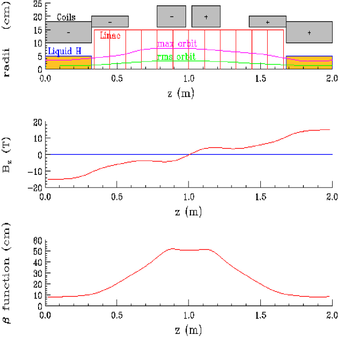
Figure 23 shows the cross section of one cell of such a system, together with the betatron function, and the magnetic field along the axis. For convenience in modeling, the section shown in Fig. 23(a) starts and ends symmetrically in the middle of hydrogen absorber regions at the location of the peaks in the axial magnetic field. In practice each cell would start at the beginning of the hydrogen region and extend to the end of the rf module.
A GEANT simulation of muons traversing a section of the cooling channel is shown in Fig. 24.
Additional simulations were performed [151, 158] using the program ICOOL. The only likely significant effects which are not yet included are space charge and wakefields. Analytic calculations for particle bunches in free space indicate that these effects should, for the later stages, be significant but not overwhelming.
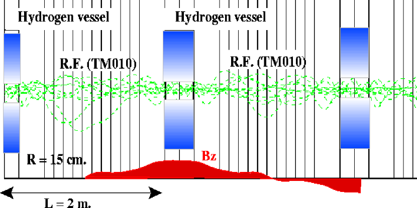
A full simulation must be done before we are assured that no problems exist. Particles are introduced with transverse and longitudinal emittance (186 MeV/ 1400 mm-mrad transverse, and 1100 mm longitudinal), together with a number of naturally occurring correlations. Firstly, the particles are given the angular momentum appropriate for the starting axial magnetic field. Secondly, particles with large initial radius and/or divergence have longer pathlengths in a solenoidal field and tend to spread out with time. This can be parameterized by defining an initial transverse amplitude
| (27) |
The temporal spreading can be minimized by introducing an initial correlation between and that equalizes the forward velocity of the initial particles. This correlation causes the average momentum of the beam to grow from the reference value of 186 MeV/ to MeV/ Lastly, a distortion of the longitudinal bunch distribution can be introduced to reflect the asymmetric nature of the “alpha”-shaped rf bucket.
Figure 25(a) shows the average momentum of the beam as a function of distance along the channel. The momentum drops as the beam crosses the liquid hydrogen absorbers. The gradient and phase of the rf cavities have been adjusted so that the reacceleration given to the reference particle equals the mean energy loss. This causes the average momentum of the beam to remain in a narrow band around 195 MeV/ Figure 25(b) shows the mechanical and canonical angular momenta as a function of distance along the channel. The mechanical angular momentum shows the rotational motion of the beam around the axial solenoidal field. It periodically reverses sign when the solenoids alternate direction. The canonical angular momentum is defined such that it removes the axial field dependence [158]. Without the absorbers, the beam would have a constant (0) value for the canonical angular momentum. However, the presence of absorbers causes the canonical angular momentum to grow and would lead to severe emittance growth by the end of a long channel. This growth is stopped by alternating the direction of the solenoid field, as shown in Fig. 25(b) Simulations have shown that 2 m is a reasonable (half) period for the field, since the net growth in canonical angular momentum is small. In addition synchrobetatron resonances are avoided since the periodicity of the field forces the average betatron wavelength to be 2 m, whereas the synchrotron oscillation wavelength seen in the simulations for this arrangement is m.
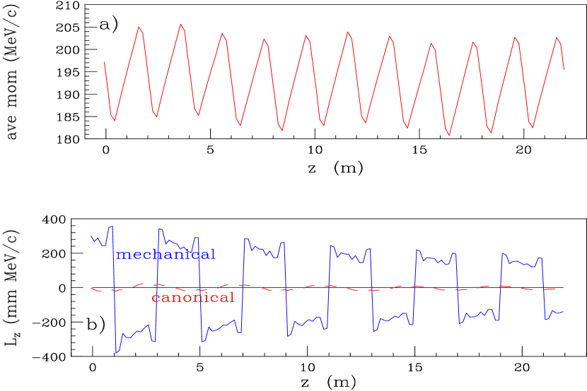
Figure 26(a) shows the rms and maximum radius of any particle in the beam distribution as a function of distance along the channel. The rms radius shows that most of the beam is confined to within 2 cm of the axis. The peak rms radius decreases towards the end of the channel as a result of the cooling. The maximum particle radius is about 8 cm, which determines the radius of the windows required in the rf cavities. Figure 26(b) shows the rms momentum spread corrected for the correlation between and transverse amplitude imposed on the initial particle distribution. The momentum spread grows as a function of distance since the alternating solenoid system only cools the transverse emittance. Figure 26(c) shows the rms bunch length s a function of distance along the channel. Again this grows with distance since this channel does not cool longitudinally.
Figure 27(a) shows the decrease in transverse normalized emittance as a function of distance along the channel. The system provides cooling by a factor of 2 in both the and transverse phase spaces. From the changing slope of the curve we note that the rate of cooling is dropping. This sets 22 m as the maximum useful length for this type of system. It must be followed by a longitudinal emittance exchange region to reduce the momentum spread and bunch length approximately back to their starting values. Figure 27(b) shows the increase in longitudinal normalized emittance in the channel due to the increase in momentum spread and bunch length. Finally, Fig. 27(c) shows the decrease in the 6-D normalized emittance as a function of distance along the channel. There is a net decrease in 6-D emittance by a factor of 2 in the channel. Table V gives the initial and final beam parameters.
| initial | final | final/initial | ||
|---|---|---|---|---|
| Particles tracked | 1000 | 980 | 0.98 | |
| Reference momentum | MeV/ | 186 | 186 | 1.0 |
| Transverse Emittance | mm-mrad | 1400 | 600 | 0.43 |
| Longitudinal Emittance | mm-mrad | 1100 | 2300 | 2.09 |
| 6-D emittance | ( m-rad)3 | 2000 | 800 | 0.40 |
| rms beam radius in hydrogen | cm | 0.8 | 0.55 | 0.69 |
| rms beam radius in linac | cm | 2.0 | 1.4 | 0.70 |
| max beam radius in linac | cm | 7.0 | 7.0 | 1.0 |
| rms bunch length | cm | 1.5 | 2.2 | 1.5 |
| max bunch full width | cm | 13 | 19 | 1.5 |
| rms | % | 3.8 | 5.6 | 1.5 |
E 31 T solenoid transverse cooling example
As in the preceding example, the lattice consists of 11 identical 2 m long cells with the direction of the fields in the solenoids alternating from one cell to the next. The maximum solenoidal field is higher (31 T) than in the previous example, but the bore is smaller (8 cm), and the liquid hydrogen absorber has a smaller diameter (6 cm). Between the 31 T solenoids there are 1.3 m long matching sections with an inside diameter of 32 cm, superimposed on a 36 MeV/m reacceleration linac operating at 805 MHz.
Table VI gives the initial and final parameters for the 31 T example, together with the required emittances for a Higgs factory. In setting these requirements a dilution of during acceleration is assumed in each of the three emittances.
| initial | final | final/initial | required | ||
|---|---|---|---|---|---|
| Particles tracked | 4000 | 3984 | 0.99 | ||
| Reference momentum | MeV/ | 186 | 186 | ||
| Transverse Emittance | mm-mrad | 460 | 240 | 0.52 | 240 |
| Longitudinal Emittance | mm-mrad | 850 | 1600 | 1.9 | |
| 6-D emittance | ( m-rad)3 | 150 | 95 | 0.63 | 98 |
| rms beam radius in hydrogen | cm | 0.44 | 0.33 | 0.75 | |
| rms beam radius in linac | cm | .4 | 1.1 | 0.80 | |
| max beam radius in linac | cm | 6.0 | 6.0 | 1.0 | |
| rms bunch length | cm | 1.5 | 1.8 | 1.2 | |
| max bunch full width | cm | 11 | 19 | 1.7 | |
| rms | % | 3.5 | 5.0 | 1.4 |
F Bent solenoid emittance exchange example
We have been considering using a system that exchanges longitudinal and transverse emittance by exploiting dispersion in a large acceptance channel, with a low-Z wedge absorber in the region of dispersion.
In a bent solenoid, in the absence of any dipole field, there is a drift perpendicular to the bend plane of the center of the Larmor circular orbit, which is proportional to the particle’s momentum [159]. In our example we have introduced a uniform dipole field over the bend to cancel this drift exactly for particles with the reference momentum. Particles with momenta differing from the reference momentum then spread out spatially, giving the required dispersion (0.4 m). The dispersion is removed, and the momentum spread reduced, by introducing liquid hydrogen wedges [160]. The hydrogen wedges would be contained by thin beryllium or aluminum foils, but these were not included in this simulation.
After one bend and one set of wedges, the beam is asymmetric in cross section. Symmetry is restored by a following bend and wedge system rotated by 90 degrees with respect to the first. Figure 28 shows a representation of the two bends and wedges. The total solenoid length was 8.5 m. The beam tube outside diameter is 20 cm, and the minimum bend radii is 34 cm.
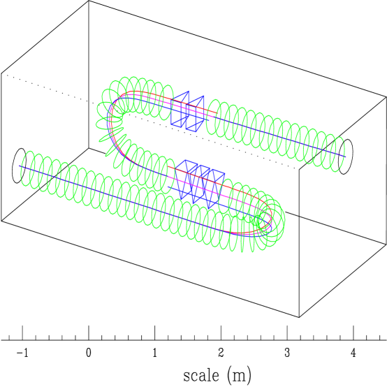
Figure 29(a) shows the magnetic fields (Bz, By, and Bx) as a function of the position along the cell. The solenoid bend curvature is exactly that given by the trajectory of a reference particle (equal in momentum to the average momenta given in Fig. 29(b)) in the given transverse fields. The actual shape of the bend turns out to be very important. Discontinuities in the bend radius can excite perturbations which increase the transverse emittance. We have shown, for example, that the transverse emittance growth in a bent solenoid depends on discontinuities of the bend radius as a function of distance, and its first and second derivatives, the size and tilt of the solenoidal coils, auxiliary fields and the 6-D phase space of the beam. Thus optimization is not straightforward. One solution to this problem is to have long, adiabatic bends. However, this adds undesirable length to the emittance exchange section. We are studying options with coupling sections to tight bends roughly half a Larmor length long, which seems to minimize transverse emittance growth while also minimizing the length of the section. Due to similar problems, the length and longitudinal distribution of the wedge material has also been found to affect emittance growth. For example, the growth can be minimized when the vector sum of the Larmor phases at the absorber elements is small or zero.
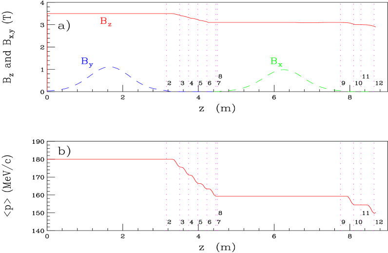
The simulations were performed using the program ICOOL. The maximum beam radius is 10 cm. Transmission was 100%. Figure 30(a) shows the rms longitudinal momentum spread relative to the reference momentum as a function of the position along the cell. The fractional spread decreases from an initial value of approximately 5%, to a final value of approximately 2.2%. At the same time, since this is an emittance exchange, the transverse beam area grows, as shown in Fig. 30(b). One notes that the area increases not only in the regions of bends (region 1 and 8), but also in the regions of wedges (2-6 and 9-11). This is probably due to failures in matching that have yet to be understood.
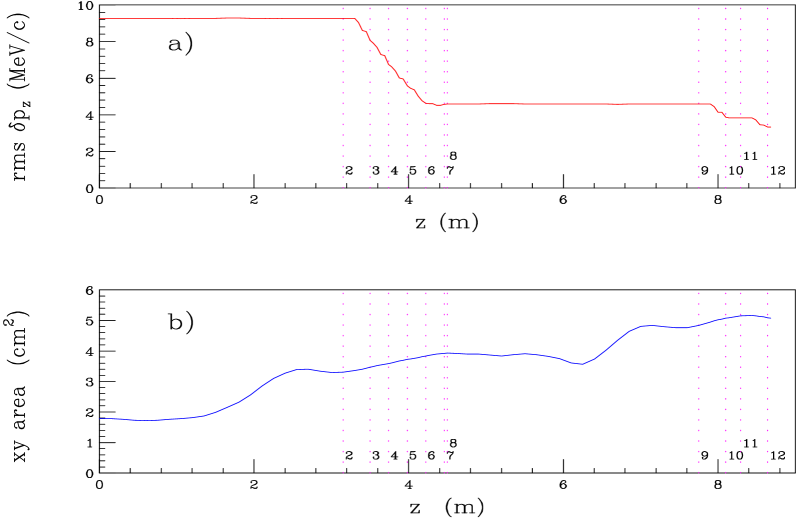
Figure 31 shows scatter plots of the transverse particle positions against their momenta. The dispersion is clearly observed in Fig. 31(b) (after the first bend) and in Fig. 31(e) (after the second). It is seen to be removed, with a corresponding decrease in momentum spread, in Fig. 31(c) (after the first set of wedges) and Fig. 31(f) (after the second set of wedges).
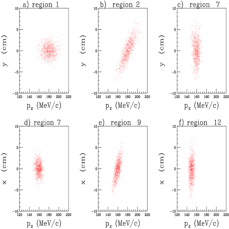
Figure 32 shows a scatterplot of the square of the particle radii vs. their longitudinal momenta, (a) at the start, and (b) at the end of the emittance exchange section. The decrease in momentum spread and rise in beam area are clearly evident.
The initial and final beam parameters are given in table VII. Although this example demonstrate a factor of reduction in the longitudinal momentum spread, there is a increase in the 5-D phase space. The simulations must be extended to include rf so that the 6-D emittance can be studied and the emittance exchange section can be optimized.
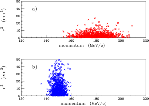
| initial | final | final/initial | ||
| Longitudinal Momentum spread | MeV/ | 9.26 | 3.35 | 0.36 |
| Ave. Momentum | MeV/ | 180 | 150 | 0.83 |
| Transverse size | cm | 1.33 | 2.26 | 1.70 |
| Transverse Momentum spread | MeV/ | 6.84 | 7.84 | 1.15 |
| Transverse Emittance | mm-mrad | 870 | 1694 | 1.95 |
| Emit p | ( m-mrad)2 MeV/ | 7.0 | 9.6 | 1.37 |
G RF for the cooling systems
The losses in the longitudinal momentum of the muon beam from the cooling media have to be restored using rf acceleration sections. These rf structures are embedded in solenoidal fields that reverse direction within each section. In the two transverse cooling examples above, the rf frequency is 805 MHz and the peak gradient is 36 MeV/m. The magnetic fields that extend over the cavities vary from 0 to 10 T, reversing in the center. It should be pointed out that in the earlier stages, the bunches are longer, and lower frequencies will be required.

In order to realize maximum accelerating gradients within the acceleration cavities, we take advantage of the penetrating properties of a muon beam by placing thin windows between each rf cell, thereby creating an accelerating structure closely approximating the classic pill-box cavity. This permits operating conditions in which the axial accelerating field is equal to the maximum wall field and gives a high shunt impedance.
The windows in the 15 T example are 16 cm diameter, m thick Be foils. In the 31 T case, they are 10 cm diameter and m thick.
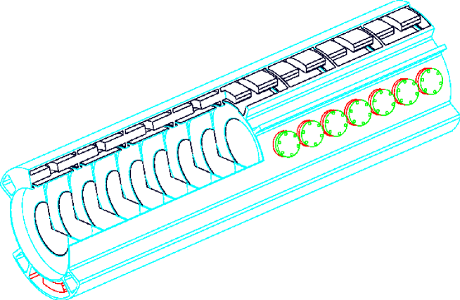
For these rf structures, we will use an interleaved cavity design in which two parts are independently powered (Fig. 33). The mode of the system will be referred to as /2 interleaved. Each section supports a standing wave mode, with each acceleration cell /2 long, giving a good transit time factor. To reduce the peak rf power requirements (by a factor of 2), we are considering operating the cells at liquid nitrogen temperatures.
| RF frequency [MHz] | 805 |
|---|---|
| Cavity Length [cm] | 8.1 |
| Cavity Inner Radius [cm] | 14.6 |
| Cavity Outer Radius [cm] | 21 |
| 2 20 | |
| Peak Axial Gradient [MV/m] | 36 |
| Shunt Impedance [M/m] | |
| [M/m] | |
| Fill Time (3 ) [s] | |
| RF Peak Power [MW/m] | |
| Ave. Power (15Hz) [KW/m] | 5.3 |
| Be window aperture [cm] | 16 (10 for 31 T case) |
| Be window thickness [m] | 127 (50 for 31 T case) |
H The liquid lithium lens
The final cooling element ultimately determines the luminosity of the collider. In order to obtain smaller transverse emittance as the muon beam travels down the cooling channel, the focusing strength must increase, i.e. the ’s must decrease. A current within a conductor produces an active lens absorber, which can maintain the beam at small throughout an extended absorber length, while simultaneously attenuating the beam momentum. An active lens absorber, such as a lithium lens, may prove to be the most efficient cooling element for the final stages.
The cooling power of a Li lens is illustrated in Figure 35, where the vs. phase space distributions at the beginning and at the end of the absorber are shown. This example corresponds to a 1 m long lens, with 1 cm radius, and a surface field of 10 T. The beam momentum entering the lens was 267 MeV/ with Gaussian transverse spatial and momentum distributions: mm, MeV/ and a normalized emittance of mm-mrad. The normalized emittance at the end of the absorber was mm-mrad (cooling factor ), and the final beam momentum was 159 MeV/ The results were obtained using a detailed GEANT simulation of a single stage.
An alternative cooling scheme under study uses a series of Li lenses. The lens parameters would have to vary to match the changing beam emittance along the section and in addition, acceleration of the beam between the lenses has to be included.

Lithium lenses have been used with high reliability as focusing elements at FNAL and CERN [7, 153, 154]. Although these lenses have many similar properties to those required for ionization cooling, there are some very crucial differences which will require significant advances in lens technology: ionization cooling requires longer lenses ( 1 meter), higher fields (), and higher operation rates (15 Hz). The last requirement calls for operating the lenses with lithium in the liquid phase.
A liquid Li lens consists of a small diameter rod-like chamber filled with liquid Li through which a large current is drawn.
The azimuthal magnetic field focuses the beam to give the minimum achievable emittance where the constant depends on the properties of the material, for example, mm-mrad/cm. The focusing term can be written as [cm] with is the muon momentum in MeV/ and is the current density in MA/cm2. Increasing is obviously desirable. Decreasing can also be useful. However, below about 250 MeV/ the slope of tends to increase the longitudinal emittance. The requirement for the highest current density causes large ohmic power deposition. The current density will be limited by the maximum tolerable deposited energy, which will produce instantaneous heating, expansion, and pressure effects. Understanding these effects is part of the ongoing liquid Li lens R&D.
The structural design of the lithium lens is determined by how the pressure pulse and heat deposition are handled. We assume that the Li will be flowing rapidly under high pressure, confined by electrical insulators radially and by fairly thick Be windows longitudinally. Operation at 15 Hz for long periods poses severe challenges. Shock, fatigue and other failure modes are being evaluated, in addition to studies of material compatibilities, corrosion and degradation to insure safe operation over long periods. It seems that the minimum required radius of the lens may be the most important parameter to determine, since mechanical problems rise while losses decrease as a function of radius.
Transferring the beam from one lens to another, with linacs to reaccelerate and provide longitudinal focusing, is also a challenging problem, because of the multiple scattering introduced in the windows, straggling and the large divergence of the beams. We are in the process of evaluating a number of designs for this transfer channel, using detailed tracking simulations that include solenoids, quadrupoles and other focusing elements together with Li lenses.
A group from BINP has designed, and is constructing, a 15 cm long liquid lithium lens prototype that will eventually be tested at FNAL. It is planned to extend this R&D program to design, construct, and test longer lenses. The design of two lenses, whose behavior will be tested at first on a bench and then with muon beams at the Ionization Cooling Demonstration Facility, will then follow [163].
I Ionization cooling experimental R&D
An R&D program has been proposed to design and prototype the critical sections of a muon ionization cooling channel. The goal of this experimental R&D program is to develop the muon ionization cooling hardware to the point where a complete ionization cooling channel can be confidently designed for the First Muon Collider. Details can be found in Fermilab proposal P904 [163]. A summary of the R&D program can be found in ref. [164].
The proposed R&D program consists of:
-
Developing an appropriate rf re-acceleration structure. It is proposed to construct a 3-cell prototype rf cavity with thin beryllium windows, which will be tested at high power and within a high-field solenoid.
-
Prototyping initially a 2 m section, and eventually a 10 m section, of an alternating solenoid transverse cooling stage. It is proposed to test the performance of these sections in a muon beam of the appropriate momentum.
-
Prototyping an emittance exchange (wedge) section and measuring its performance in a muon beam of the appropriate momentum.
-
Prototyping and bench testing m long liquid lithium lenses, and developing lenses with the highest achievable surface fields, and hence the maximum radial focusing.
-
Prototyping a lithium lens–rf–lens system and measuring its performance in a muon beam of the appropriate momentum.
-
Developing, prototyping, and testing a hybrid lithium lens/wedge cooling system.
The measurements that are needed to demonstrate the cooling capability and optimize the design of the alternating solenoid, wedge, and lithium lens cooling stages will require the construction and operation of an ionization cooling test facility. This facility will need
-
1.
a muon beam with a central momentum that can be chosen in the range - MeV/
-
2.
an experimental area that can accommodate a cooling and instrumentation setup of initially m in length, and eventually up to m in length, and
-
3.
instrumentation to precisely measure the positions of the incoming and outgoing particles in 6-D phase space and confirm that they are muons.
In the initial design shown in Fig. 36, the instrumentation consists of identical measuring systems before and after the cooling apparatus [165]. Each measuring system consists of (a) an upstream time measuring device to determine the arrival time of the particles to one quarter of an rf cycle ( ps), (b) an upstream momentum spectrometer in which the track trajectories are measured by low pressure TPC’s on either side of a bent solenoid, (c) an accelerating rf cavity to change the particles momentum by an amount that depends on its arrival time, (d) a downstream momentum spectrometer, which is identical to the upstream spectrometer, and together with the rf cavity and the upstream spectrometer forms a precise time measurement system with a precision of a few ps. The measuring systems are 8 m long, and are contained within a high-field solenoidal channel to keep the beam particles within the acceptance of the cooling apparatus.
It is proposed to accomplish this ionization cooling R&D program in a period of about 6 years. At the end of this period we believe that it will be possible to assess the feasibility and cost of constructing an ionization cooling channel for the First Muon Collider, and if it proves feasible, begin a detailed design of the complete cooling channel.
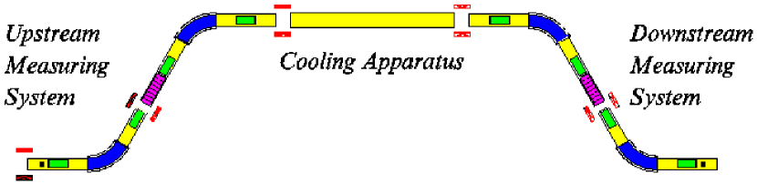
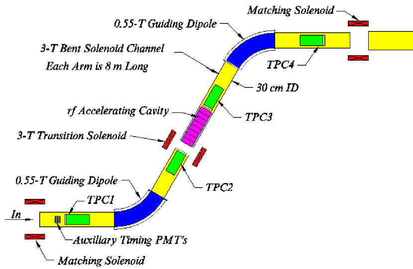
VI ACCELERATION
A Introduction
Following cooling and initial bunch compression, the beams must be rapidly accelerated. In this section some of the options in accelerator design will be described and examples of acceleration scenarios presented.
Separate acceleration scenarios are given here for a low momentum spread 100 GeV First Muon Collider (Higgs factory), and for a high luminosity 3 TeV collider. Ideally, though more difficult, this accelerator designed for the low energy machine should be extendable to the GeV beam energy and from there to the TeV beam energy needed for a very high-energy collider.
While acceleration of muons to high energy is clearly possible, an optimal and cost-effective acceleration complex is needed. In the scenarios described below, a low-frequency linac would take the beam from the end of cooling to an energy of 1 GeV followed by recirculating-linac systems to take the beam to 50-70 GeV. The multi-TeV energy regime can be reached through a series of very rapid cycling synchrotrons. Variations on the acceleration model and potential difficulties are discussed, including the use of Fixed Field Alternating Gradient (FFAG) accelerators in place of, or together with, the recirculating-linacs. Finally, topics for further study and research are described.
B Accelerator options
The acceleration time is limited by muon decay ( at rest) and requires that:
where is the acceleration rate. An acceleration rate whose value of 0.16 MeV/m is low for a linac, but very high for a conventional synchrotron.
At the lowest energies ( 700 MeV), the momentum spread and beam sizes are so large that only a linac is feasible, and acceleration to full energy in a single-pass linac would be good, but it would be very expensive.
Thus, following the initial linac, some form of recirculating acceleration is preferred. A synchrotron would be possible, in principle, but the acceleration must occur so rapidly that conventional magnet ramping is unlikely to be practical. Two alternative multi pass methods are being considered: recirculating linac accelerators similar to those used at TJNAF and Fixed Field Alternating Gradient (FFAG) accelerators.
In a recirculating linac accelerator, the beam is circulated through the same linac for several passes, with separate, energy matched, fixed-field return paths for each pass. Each return path is optically independent and can be separately designed. In the initial lattice design for the muon recirculating linac accelerator, the return arcs are similar alternating gradient (AG) systems with the same dipole layout, but with differing quadrupole strengths to allow separate tuning and chronicity matching in each arc. Multiple aperture superconducting magnets have also been designed which would reduce the diameter of the recirculating linac, lowering muon loss from decay and possibly being more economical (see Fig 7.12 [44]). In either case, both the linac and return transports must accommodate large transverse emittances (rms) of mm-mrad. Strong focusing is required not only to keep apertures down, but also to minimize orbit deviations due to the large momentum spreads, which in the initial stages of acceleration, can be as large as 10% rms.
More recently, an adaptation of the FFAG (Fixed-Field Alternating Gradient) accelerator concept has been proposed for acceleration [166, 167]. In this variation, return transports are designed with a very large (factor of 5-10) energy acceptance, so that separate energy turns can pass through the same fixed-field elements. More acceleration turns are possible than with a recirculating linac accelerator which reduces the rf requirements; but the orbits and focusing properties are now energy-dependent. Such FFAG configurations require strong superconducting magnets with large apertures to accommodate the energy-dependent spread in closed orbits. The extra cost associated with increased magnet apertures must be evaluated against potential savings in the number of magnets and reduced rf/turn requirements.
For the higher energy stages, the muon life time is greater and the needed rate of energy increase is less. Thus, above a few hundred GeV, rapid accelerating synchrotrons become possible. In a rapid accelerating synchrotron, the beam is also multi-pass accelerated through an rf system, but the beam returns in a single arc, as the magnetic field is ramped to match the increase in beam energy. As above, more acceleration turns are possible than with a recirculating accelerator, but we now have a single moderate aperture return transport. But rapid cycling synchrotrons have higher power costs and the technical challenges associated with the rapid acceleration time needed to conserve muons.
Thus a complete system would likely include an initial linac followed by a sequence of recirculating linac accelerators and/or Fixed Field Alternating Gradient machines. Depending on the final collider energy, one or more rapid acceleration synchrotrons would follow. Each system increases the beam energy by a factor of 5-10.
C Scenario examples
Several scenarios have been discussed earlier [168, 169], see for instance the parameters (table XI) used in a simulation of longitudinal motion discussed below. The ones given here are more recent, and more detailed, but they should not be taken to be definitive. They are examples that were derived to probe the design problems and to show that solutions should be possible.
1 Acceleration for Higgs collider
Table IX gives an example of a sequence of accelerators for a 100 GeV Higgs Factory, i.e. a machine with very low momentum spread (0.003%, see table I) and relatively large rms transverse emittance ( mm-mrad).
Following initial linacs, recirculating accelerators are used. The number of arcs in each recirculating accelerator is about 10. In this example, conventional fixed field 2 T magnets are used, but the effective ramp frequencies that would be needed if pulsed magnets were used are given for reference.
| Acc. type | linac | linac | recirc | recirc | recirc | sums | |
|---|---|---|---|---|---|---|---|
| Magnet type | warm | warm | warm | ||||
| rf type | Cu | Cu | Cu | Cu | Cu | ||
| (GeV) | 0.10 | 0.20 | 0.70 | 2 | 7 | ||
| (GeV) | 0.20 | 0.70 | 2 | 7 | 50 | ||
| Circ. | (km) | 0.04 | 0.07 | 0.07 | 0.19 | 1.74 | 2.11 |
| Turns | 1 | 1 | 8 | 10 | 11 | ||
| Loss | (%) | 2.31 | 3.98 | 7.27 | 7.91 | 13.94 | 31.06 |
| Decay heat | (W/m) | 0.89 | 1.98 | 11.04 | 12.99 | 12.44 | |
| (T) | 2 | 2 | 2 | ||||
| Ramp freq. | (kHz) | 281 | 79.83 | 8.00 | |||
| Disp | (m) | 1 | 1.50 | 3 | |||
| (m) | 0.83 | 1.42 | 3.00 | 5.31 | 21.08 | ||
| (cm) | 2.71 | 2.22 | 1.42 | 1.64 | 0.90 | ||
| (%) | 3.58 | 2.80 | 1.64 | 0.56 | 0.32 | ||
| (cm) | 1.09 | 1.14 | 1.01 | 0.85 | 0.94 | ||
| (cm) | 1.93 | 1.19 | 1.34 | ||||
| Pipe full height | (cm) | 10.92 | 11.42 | 10.14 | 8.49 | 9.39 | |
| Pipe full width | (cm) | 10.92 | 11.42 | 19.28 | 11.94 | 13.35 | |
| rf freq. | (MHz) | 200 | 200 | 200 | 200 | 400 | |
| Acc/turn | (GeV) | 0.20 | 0.40 | 0.17 | 0.50 | 4 | |
| Acc time | () | 1 | 6 | 62 | |||
| (%) | 5.15 | 5.36 | 6.36 | 2.84 | 6.92 | ||
| Acc. Grad. | (MV/m) | 8 | 8 | 8 | 10 | 10 | |
| Synch. rot’s | 0.62 | 0.63 | 0.62 | 3.92 | 23.16 | ||
| Cavity rad. | (cm) | 54.37 | 54.88 | 54.88 | 60.47 | 38.26 | |
| Beam time | (ms) | 0.00 | 0.00 | 0.00 | 0.01 | 0.06 | |
| rf time | (ms) | 0.17 | 0.17 | 0.17 | 0.18 | 0.13 | |
| Tot. peak rf | (GW) | 0.05 | 0.10 | 0.05 | 0.26 | 4.71 | 5.17 |
| Ave. rf power | (MW) | 0.14 | 0.24 | 0.13 | 0.68 | 9.54 | 10.73 |
| rf wall | (MW) | 0.64 | 1.16 | 0.46 | 2.42 | 28.06 | 32.75 |
In this example, all the accelerating cavities are room temperature copper structures, and the accelerating gradients are modest ( MeV/m). Nevertheless, the acceleration is rapid enough that the total losses from decay are only 30%. The heating from these decays is also modest ( W/m) because of the small number of turns and relatively low energy. Since no superconducting magnets or rf are used in this example, this heating should cause no problem.
In this machine, the transverse emittances are large and strong focusing is thus required, but the maximum momentum spread is moderate (up to 1.37 rms in the first recirculator) and is thus not likely to be a problem.
If the same machine is to also run at a high luminosity, with larger momentum spread, then although the six dimensional emittance is the same as in the Higgs collider discussed above, the transverse emittance is smaller ( mm-mrad rms ), and the longitudinal emittance larger (by about a factor of 4) and the momentum spread in the first recirculating accelerator would be nearly 6% rms; or about 50% full width. This is a very large momentum spread that could only be accepted in FFAG like lattices as discussed below.
Similarly, if the same acceleration is to be usable as the front end for a 250 + 250 GeV or higher energy machine then the transverse emittance will again be less, the longitudinal emittance even larger, and the problem of very large momentum spread will be worse. Clearly, although not absolutely needed for a Higgs Factory, it is desirable to solve this problem even in that First Collider.
A separate parameter set for the high luminosity 50 + 50 GeV collider and a 250 + 250 GeV collider could have been presented, but their parameters are very similar to those of the front end of the 3 TeV machine given below, and are thus omitted here.
2 Acceleration for 3 TeV collider
For a high energy machine, the muon accelerators are physically the largest component and are also probably the most expensive. More work is needed on its design. Table X gives an early example of a possible sequence of accelerators for a 3 TeV collider.
Linacs are used up to 700 MeV, followed by recirculating linac accelerators. In the first of these, because of the very large longitudinal emittance, the momentum spread as the beam enters the first recirculating linac accelerator is 8.5% rms, which is very large. The lattice must have very strong focusing, small dispersion and large aperture. If this is not possible, higher energy linacs or lower frequency rf could relieve the requirement.
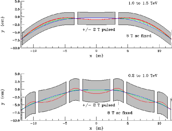
For the final three stages, pulsed magnet synchrotrons [170] are used. In the 200 GeV ring, all the magnets in the ring are pulsed, but in the last two rings a superconducting-pulsed hybrid solution is used. In these cases, if only pulsed magnets were used, then the power consumed would be too high, and because only low pulsed fields could be used, the circumferences would also be very large. It is thus proposed to use rings with alternating warm pulsed magnets and superconducting fixed magnets [171] (see figure 37). The fixed magnets are superconducting at 8 T; the pulsed magnets are warm with fields that swing from - 2 T to + 2 T. The effective ramp frequency is given in the table. Both of these rings are in the same tunnel, with the fraction of magnet length pulsed (vs. fixed) being different (73% and 43%).
In all the final three rings superconducting rf is employed to minimize the peak power requirements and to obtain high wall to beam efficiency and thus keep the wall power consumption reasonable. In the final two rings the frequency and cavity designs are chosen to be the same as that in the TESLA [172] proposal.
| Acc. type | linac | recirc | recirc | recirc | synch | synch | synch | sums | |
|---|---|---|---|---|---|---|---|---|---|
| Magnet type | warm | warm | warm | warm | hybrid | hybrid | |||
| rf type | Cu | Cu | Cu | SC Nb | SC Nb | SC Nb | SC Nb | ||
| (GeV) | 0.10 | 0.70 | 2 | 7 | 50 | 200 | 1000 | ||
| (GeV) | 0.70 | 2 | 7 | 50 | 200 | 1000 | 1500 | ||
| Circ. | (km) | 0.07 | 0.12 | 0.26 | 1.74 | 4.65 | 11.30 | 11.36 | 29.52 |
| Turns | 2 | 8 | 10 | 11 | 15 | 27 | 17 | ||
| Loss | (%) | 6.11 | 12.28 | 10.84 | 13.94 | 10.68 | 10.07 | 2.65 | 50.58 |
| Decay heat | (W/m) | 3.67 | 15.02 | 16.89 | 15.91 | 19.44 | 30.97 | 18.09 | |
| (T) | 2 | 2 | 2 | ||||||
| (T) | 0.70 | 1.20 | 2 | 8 | 8 | ||||
| frac pulsed | % | 73 | 43 | ||||||
| Ramp freq. | (kHz) | 162 | 57.34 | 8.00 | 2.15 | 0.50 | 0.79 | ||
| Disp. | (m) | 0.40 | 0.60 | 0.80 | 1 | 2 | 4 | ||
| (m) | 0.89 | 3.97 | 8.75 | 36.29 | 52.20 | 108 | 120 | ||
| Mom. compactn | % | 1 | -0.25 | -0.50 | -0.50 | -0.50 | -1 | ||
| (cm) | 16.34 | 8.53 | 5.29 | 3.57 | 1.59 | 0.96 | 0.78 | ||
| (%) | 19.27 | 8.49 | 5.41 | 2.47 | 0.82 | 0.35 | 0.09 | ||
| (cm) | 0.45 | 0.45 | 0.42 | 0.48 | 0.22 | 0.16 | 0.08 | ||
| (cm) | 3.40 | 3.25 | 1.98 | 0.82 | 0.71 | 0.36 | |||
| Pipe full height | (cm) | 4.46 | 4.52 | 4.22 | 4.77 | 2.20 | 1.62 | 0.78 | |
| Pipe full width | (cm) | 4.46 | 33.95 | 32.49 | 19.79 | 8.20 | 7.06 | 3.62 | |
| rf Freq | (MHz) | 200 | 100 | 200 | 200 | 800 | 1300 | 1300 | |
| Acc./turn | (GeV) | 0.40 | 0.17 | 0.50 | 4 | 10 | 30 | 30 | |
| Acc. time | () | 3 | 8 | 62 | 232 | 1004 | 631 | ||
| (%) | 3.82 | 0.96 | 1.97 | 1.11 | 10.15 | 14.37 | 12.92 | ||
| Acc. Grad. | (MV/m) | 8 | 8 | 10 | 10 | 15 | 25 | 25 | |
| Synch. rot’s | 0.81 | 0.76 | 1.02 | 5.82 | 19.14 | 54.29 | 31.30 | ||
| Cavity rad. | (cm) | 54.88 | 110 | 60.47 | 76.52 | 19.13 | 11.77 | 11.77 | |
| rf time | (ms) | 0.04 | 0.12 | 0.05 | 0.56 | 0.40 | 1.25 | 0.96 | |
| Tot. peak rf | (GW) | 0.21 | 0.14 | 0.59 | 1.31 | 1.06 | 1.16 | 1.04 | 5.51 |
| Ave. rf power | (MW) | 0.14 | 0.25 | 0.45 | 11.04 | 6.32 | 21.91 | 15.07 | 55.18 |
| rf wall | (MW) | 0.64 | 0.88 | 1.62 | 32.47 | 18.59 | 44.72 | 30.76 | 130 |
D Design issues
1 Recirculating linac accelerator lattice issues
Beam transport R&D for recirculating linac accelerators follows the model of the Thomas Jefferson National Accelerator Facility (TJNAF). The layout is a racetrack with linacs in the straight sections and multi-pass return arcs. At the ends of the linacs the multi-pass beam lines are recombined. A pulse magnet at each separation/recombination point is used to guide the beam into the energy matched return arc. Some initial lattice design concepts for recirculating linac accelerators are being developed. The basic return arc unit would be a FODO lattice, but with the quadrupole strengths varied in order to perturb the arc dispersion function and obtain nearly isochronous motion around the arcs. The arcs are dispersion matched by setting the arc phase advance to a multiple of 2. Arc designs based upon the flexible momentum compaction (FMC) module can also be used.
In the special case of the very low momentum spread Higgs factory, the transverse emittances are very large ( mm-mrad rms), and will require strong focusing in the lattices. Momentum acceptance in the rings is, in this case, not a problem. But the longitudinal phase space of the muons in the other machines is much larger and requires, at low energies, either long bunches, or large momentum spreads. The requirement of high accelerating gradients argues for high frequencies, and thus short bunches. One therefore needs accelerators with large momentum acceptances.
In the 3 TeV example above, the acceptance at injection into the first recirculating accelerator is 8.5% rms. This is very large by conventional standards, but far less than that in the FFAG lattices being studied [166]. Thus the early return arcs of such a recirculating linac accelerator would have to have very strong focusing, and be FFAG-like. Of course, if a true FFAG accelerator were to be used for its avoidance of the switchyards and multi-aperture magnets, then the specified momentum spread would certainly not be a problem.
Permanent, ferric or superferric (2 T), or high field superconducting magnets could be used for recirculating linac accelerators. The lower field magnets may be economic for initial turns, while high field magnets minimize particle travel times, and therefore decay losses. Designs for multi-aperture superconducting magnets suitable for recirculating linac accelerators have been developed [44], and superconducting magnets with as many as 18 apertures with 0.7–7 T fields have been designed. A variety of magnet configurations can be developed; cost/performance optimization will be needed in developing a final choice.
2 RF peak power requirements
Because of the need for rapid acceleration, the peak rf powers are high, and the resulting numbers of power sources large. For the linacs and early recirculating accelerators, the powers are high because of the high gradients and low frequencies needed to accelerate the long bunches. At these frequencies (200 MHz), currently available sources (triodes and tetrodes) have relatively low maximum output powers and are expensive. Low temperature operation of the cavities, and superconducting or conventional SLED [173] systems, which would reduce the peak power requirements, are being considered.
Study of the example suggests that in the first two recirculators (up to 7 GeV) there is no hope for the rf to keep up with the beam loading. The cavity can only be filled in a suitable filling time (twice the time constant in these examples), and the rf voltage allowed to sag as the beam makes its multiple passes. If excessive sensitivity to beam current is to be avoided, then the stored energy must be large compared to that used, which is somewhat inefficient.
In the final recirculating accelerator, continuous filling (cw) is just possible, but requires yet higher peak power ( GW total at 400 MHz) because of the high acceleration rate. The use of superconducting cavities can reduce losses, and thus reduce this peak rf power source requirement, and was included in the above 3 TeV example. At this frequency (400 MHz), klystrons are available with greater power ( MW) than that of the sources at the lower frequencies, but a yet higher power klystron (50-100 MW) could probably be developed and would be desirable.
3 Pulsed magnet systems
A pulsed current 4 T magnet has been designed for acceleration to 250 GeV in 360 s [174], but efficiency favors use of ferric materials in rapid acceleration magnets, although this would limit peak magnetic fields to 2 T. The average field can be increased by interleaving magnets swinging from -2 T to 2 T with fixed field 8 T superconducting magnets.
Faster pulsing magnets would require special materials to minimize energy losses from eddy currents. Options include silicon steel, metglass laminations, or finemet laminated tape or powdered solid. A 30 metglass lamination suitable for several kHz cycling has been developed. A design of suitable pulsed magnets [171](see Fig. 38) has been shown to have sufficiently low losses for this application. The magnets employ cables made of many fine insulated strands (litz cable) and the yokes are made of very thin (0.28 mm), 3% Si-Fe laminations, possibly of metglas [175, 176] for the higher rate cases. Detailed designs must be developed and prototypes constructed and the practical limits of recycling scenarios should be determined.
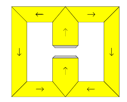
4 Superconducting linacs
While the gradients needed in the acceleration systems are not excessive, they are larger than previous experience at the lower frequencies. The high peak power pulsed operation poses power handling difficulties at lower energies and high peak current presents collective effect (wakefield) difficulties at higher energies. Higher gradients and efficiencies in all sections would improve performance.
The superconducting rf would operate in pulsed mode, matched to the acceleration time of up to a few ms. This pulse structure is similar to the multibunch acceleration mode planned for TESLA (25 MV/m at 1300 MHz designs), and studies indicate that this design could be adapted to acceleration. At lower frequencies, structures such as the CERN 350 MHz superconducting rf cavities could be used. These cavities have been tested in pulsed mode operation, and tests indicate that pulsed acceleration fields 10 MV/m are possible [177].
The high single bunch intensities required for high intensities imply large higher order mode losses and large wakefield effects from the short, high intensity bunches. Higher order mode (HOM) load designs adapted from superconducting rf experience could be used. HOM loads and wakefields are expected to vary as and and , where is the cavity aperture, is the acceleration wavelength and is the bunch length [178, 179]. Calculations indicate that the wakefields would limit bunch intensities to with 1300 MHz superconducting rf in a recirculating linac accelerator scenario. The longitudinal dynamics is microtron-like or synchrotron-like and off-crest acceleration enables compensation of the linear part of the wakefields, with synchrotron-like phase stability [168].
E Simulations
| Linac | RLA1 | RLA2 | RCS1 | RCS2 | |
| E (GeV) | 0.1 1.5 | 1.5 10 | 10 70 | 70 250 | 250 2000 |
| frf (MHz) | 30 100 | 200 | 400 | 800 | 1300 |
| Nturns | 1 | 9 | 11 | 33 | 45 |
| Vrf(GV/turn) | 1.5 | 1.0 | 6 | 6.5 | 42 |
| Cturn(km) | 0.3 | 0.16 | 1.1 | 2.0 | 11.5 |
| Beam time (ms) | 0.0013 | 0.005 | 0.04 | 0.22 | 1.73 |
| (cm) | 50 8 | 4 1.7 | 1.7 0.5 | 0.5 0.25 | 0.25 0.12 |
| (GeV) | 0.005 0.033 | 0.067 0.16 | 0.16 0.58 | 0.58 1.14 | 1.14 2.3 |
| Loss (%) | 5 | 7 | 6 | 7 | 10 |
A study [169] followed the longitudinal motion of particles through a similar sequence of recirculating accelerators (see table XI). Cavities similar to those proposed for TESLA [172] were assumed. Figure 39
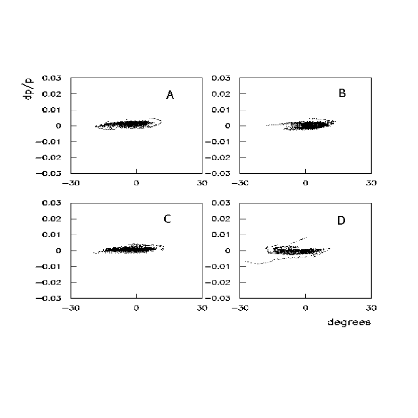
shows, after optimization of parameters, the final longitudinal phase space distributions corresponding to wakefields estimated for four different bunch charges: a) very small, b) muons, c) muons, and d) muons.
For the design beam charge of muons (approximately as for Fig. 39(c)) the wakefield amplitude was estimated to be 2.5 MV/m, the accelerating phase was 35o, and rf voltage depression 26%. The simulation used an initial longitudinal phase space of 20 eV-s. It gave negligible particle loss, a final longitudinal phase space of 21.6 eV-s, resulting in an increase of longitudinal emittance of only 8%.
F Acceleration research needed
As discussed above, possible acceleration configurations have been developed, and critical longitudinal motion simulations have been performed. These calculations support the general feasibility of acceleration of muons from cooling to collider energies. However the designs of acceleration systems have not been fully detailed and much work would be needed to obtain a buildable design. Complete transport lattices for linacs and return arcs have not yet been derived, and 6-D phase space tracking of beams through the accelerators has not been attempted. Also the geometry of combining and separating multi pass beams has not been worked out and optimized.
The rf requirements and systems have been specified at only the rudimentary requirements level, and have not been developed to a constructible level. Optimal configurations and choices of normal or superconducting rf must be developed, as well as more optimal choices in acceleration frequencies. The simple wakefield models used in the initial simulations should be expanded to obtain more realistic systems, and more precise calculations of wakefield effects must be developed.
Rapid accelerating systems have only been outlined at the simplest conceptual level. Prototype magnet design and testing are needed to test the limits of cycling rate and field strengths. Successful magnet concepts must then be specified in terms of stable beam transport configurations, including focusing and transport matching. While beam is stored for only a few turns, the individual bunch intensities are large enough that the possibility of single bunch instabilities must be considered and calculated. The larger number of passes in a recirculating linac accelerator places greater demands on the rf systems and higher order mode (HOM) loads, particularly for superconducting systems.
VII COLLIDER STORAGE RING
A Introduction
After one bunch and one bunch have been accelerated to collision energy, the two bunches are injected into the collider ring, which is a fixed field storage ring. Parameters for several possible collider storage rings are given in table I. Collider ring lattices have been developed for two of the collision energies in this table: 100 GeV and 3 TeV in the center of mass.
Three operational modes are proposed in the above table for the 100 GeV collider, each requiring different machine optics. The following sections discuss a 100 GeV collider lattice for two of the modes, the broad momentum spread case ( of , rms) and the narrow momentum spread case ( of ), as well as a 3 TeV collider lattice.
B Collider Lattices
1 Design criteria
Stringent criteria have been imposed on the collider lattice designs in order to attain the specified luminosities. The first and most difficult criterion to satisfy is provision of an Interaction Region (IR) with extremely low values at the collision point consistent with acceptable dynamic aperture. The required values for the 100 GeV collider are 4 cm for the broad momentum spread case and 14 cm for the narrow momentum spread case. For the 3 TeV machine, is only 3 mm. These values were tailored to match the longitudinal bunch lengths in order to avoid luminosity dilution from the hour-glass effect. Achieving this requirement in the 3 TeV lattice is complicated by the high peak beta function values in the final focus quadrupoles requiring 8-10 cm radial apertures. The correspondingly weakened gradients combined with the ultra-high energy make for a long final focus structure. (In contrast, the lower energy and larger values in the 100 GeV collider lead to an efficient, compact final focus telescope.) Compounding the problem, particularly for the 3 TeV design, is the need to protect the superconducting coils from the decay products of the muons. Placing a tungsten shield between the vacuum chamber and the coils can increase the radial aperture in the 3 TeV quadrupoles by as much as 6 cm, lowering available gradients still further. Final focus designs must also include collimators and background sweep dipoles, and other provisions for protecting the magnets and detectors from muon decay electrons. Effective schemes have been incorporated into the current lattices.
Another difficult constraint imposed on the lattice is that of isochronicity. A high degree of isochronicity is required in order to maintain the short bunch structure without excessive rf voltage. In the lattices presented here, control over the momentum compaction is achieved through appropriate design of the arcs.
A final criterion especially important in the lower energy colliders is that the ring circumference be as small as feasible in order to minimize luminosity degradation through decay of the muons. Achieving small circumference requires high fields in the bending magnets as well as a compact, high dipole packing fraction design. To meet the small circumference demand, 8 T pole tip fields have been assumed for all superconducting magnets, with the exception of the 3 TeV final focus quadrupoles, whose pole tips are assumed to be as high as 12 T. In addition, design studies for still higher field dipoles are in progress.
2 rf system
The rf requirements depend on the momentum compaction of the lattice and on the parameters of the muon bunch. For the case of very low momentum spread, synchrotron motion is negligible and the rf system is used solely to correct an energy spread generated through the impedance of the machine. For the cases of higher momentum spreads, there are two approaches. One is to make the momentum compaction zero to high order through lattice design. Then the synchrotron motion can be eliminated, and the rf is again only needed to compensate the induced energy spread correction. Alternatively, if some momentum compaction is retained, then a more powerful rf system is needed to maintain the specified short bunches. In either case, rf quadrupoles will be required to generate BNS [180, 181] damping of the transverse head-tail instability.
3 3 TeV CoM lattice
The 3 TeV ring has a roughly racetrack design with two circular arcs separated by an experimental insertion on one side, and a utility insertion for injection, extraction, and beam scraping on the other. The experimental insertion includes the interaction region (IR) followed by a local chromatic correction section (CCS) and a matching section. The chromatic correction section is optimized to correct the ring’s linear chromaticity, which is mostly generated by the low beta quadrupoles in the IR. In designs of e+e- colliders, it has been found that local chromatic correction of the final focus is essential [182, 183, 184, 185], as was found to be the case here. The 3 TeV IR and CCS are displayed in Fig. 40. The accompanying 3 TeV arc module in Fig 41 is an example of a module which controls momentum compaction (i.e. isochronicity) of the entire ring.
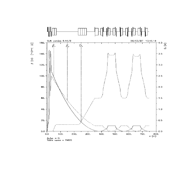
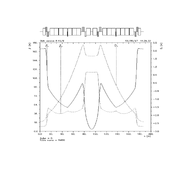
4 100 GeV CoM lattices
For the 100 GeV CoM collider [186], two operating modes are contemplated: a high luminosity case with broad momentum acceptance to accommodate a beam with a of (rms), and one with a much narrower momentum acceptance and lower luminosity for a beam with of (rms). For the broad momentum acceptance case, must be 4 cm and for the narrow momentum acceptance case, 14 cm. In either case, the bunch length must be held comparable to the value of . The 100 GeV ring geometry is highly compact and more complicated than a racetrack, but the lattice has regions with the same functions as those of the 3 TeV ring.
Two independent 100 GeV lattice designs have evolved; these are described below in separate sections and denoted Example (a) and Example (b), respectively. The first design described is a lattice which has two optics modes. In the high luminosity mode, the value is 4 cm with a transverse and momentum aperture sufficient to accept a normalized beam emittance of (rms) and a of (rms). The second, lower luminosity mode has a value of 14 cm with a very large transverse acceptance, but small, approximately monochromatic, momentum acceptance.
The second 100 GeV lattice described is another collider design with a 4 cm optics mode. Although the number of magnets differ between the two lattices, the most important optics difference between the two is in the modules used in the arcs.
5 100 GeV CoM. Example (a)
The need for different collision modes in the 100 GeV machine led to an Interaction Region design with two optics modes: one with broad momentum acceptance ( of , rms) and a collision of 4 cm, and the other basically monochromatic ( of , rms) and a larger collision of 14 cm. The first lattice design, denoted Example (a), shown in Fig. 42 and Fig. 43, has a total circumference of about with arc modules accounting for only about a quarter of the ring circumference.
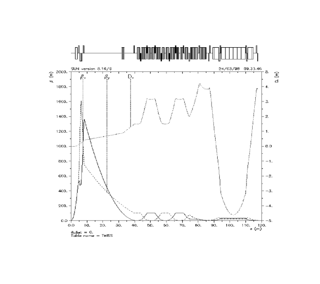
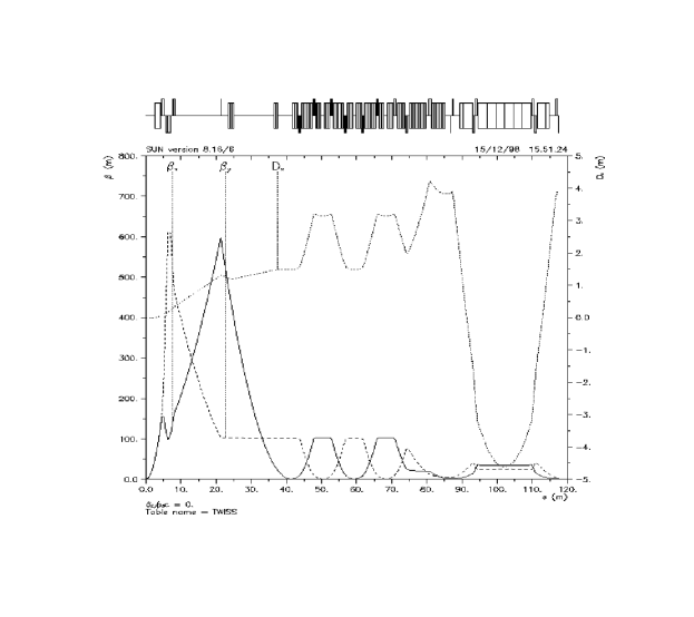
The low beta function values at the IP are mainly produced by three strong superconducting quadrupoles in the Final Focus Telescope (FFT) with pole tip fields of 8 T. The full interaction region is symmetric under reflection about the interaction point (IP). Because of significant, large angle backgrounds from muon decay, a background sweep dipole is included in the final focus telescope and placed near the IP to protect the detector and the low quadrupoles [187]. It was found that this sweep dipole, 2.5 m long with an 8 T field, provides sufficient background suppression. The first quadrupole is located 5 m away from the interaction point, and the beta functions reach a maximum value of in the final focus telescope, when the maxima of the beta functions in both planes are equalized. For this maximum beta value, the quadrupole apertures must be at least 11 cm in radius to accommodate 5 of a mm-mrad, 50 GeV muon beam (normalized rms emittance) plus a 2 to 3 cm thick tungsten liner [188]. The natural chromaticity of this interaction region is about
Local chromatic correction of the muon collider interaction region is required to achieve broad momentum acceptance. The basic approach developed by Brown [183] and others [189], is implemented in the Chromatic Correction Region (CC). The CC contains two pairs of sextupoles, one pair for each transverse plane, all located at locations with high dispersion. The sextupoles of each pair are located at positions of equal, high beta value in the plane (horizontal or vertical) whose chromaticity is to be corrected, and very low beta waist in the other plane. Moreover, the two sextupoles of each pair are separated by a betatron phase advance of near , and each sextupole has a phase separation of from the IP, where is an integer. The result of this arrangement is that the geometric aberrations of each sextupole is canceled by its companion while the chromaticity corrections add.
The sextupoles of each pair are centered about a minimum in the opposite plane (), which provides chromatic correction with minimal cross correlation between the planes. A further advantage to locating the opposite plane’s minimum at the center of the sextupole, is that this point is away from, or “out of phase” with, the source of chromatic effects in the final focus quadrupoles; i.e the plane not being chromatically corrected is treated like the IP in terms of phase to eliminate a second order chromatic aberration generated by an “opposite-plane” sextupole.
In this lattice example, the CC (Fig. 44) was optimized to be as short as possible. The is only and the , giving a between planes of about 150, so the dynamic aperture is not compromised by a large amplitude dependent tuneshift.
This large beta ratio, combined with the opposite plane phasing, allows the sextupoles for the opposite planes to be interleaved, without significantly increasing the nonlinearity of the lattice. In fact, interleaving improved lattice performance compared to that of a non-interleaved correction scheme, due to a shortening of the chromatic correction section, which lowers its chromaticity contribution [190]. The use of somewhat shallower beta minima with less variation in beta through the sextupoles was made soften the chromatic aberrations, although this caused a slight violation of the exact phase advance separation between sextupole partners. The retention of an exact phase advance difference between sextupoles was found to be less important to the dynamic aperture than elimination of minima with .
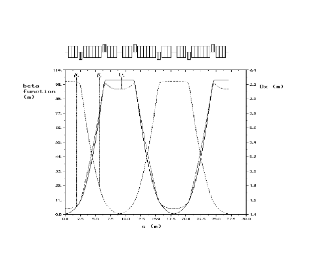
The total momentum compaction contributions of the IR, CC, and matching sections is about . The total length of these parts is , while that of the the momentum compaction correcting arc is 93 m. From these numbers, it follows that this arc must have a negative momentum compaction of about in order to offset the positive contributions from the rest of the ring.
The arc module is shown in Fig. 45. It has the small beta functions characteristic of FODO cells, yet a large, almost separate, variability in the momentum compaction of the module which is a characteristic associated with the flexible momentum compaction module [191, 192]. The small beta functions are achieved through the use of a doublet focusing structure which produces a low beta simultaneously in both planes. At the dual minima, a strong focusing quadrupole is placed to control the derivative of dispersion with little impact on the beta functions. Negative values of momentum compaction as low as have been achieved, and , has been achieved with modest values of the beta function.
This arc module was able to generate the needed negative momentum compaction with beta functions of or less.
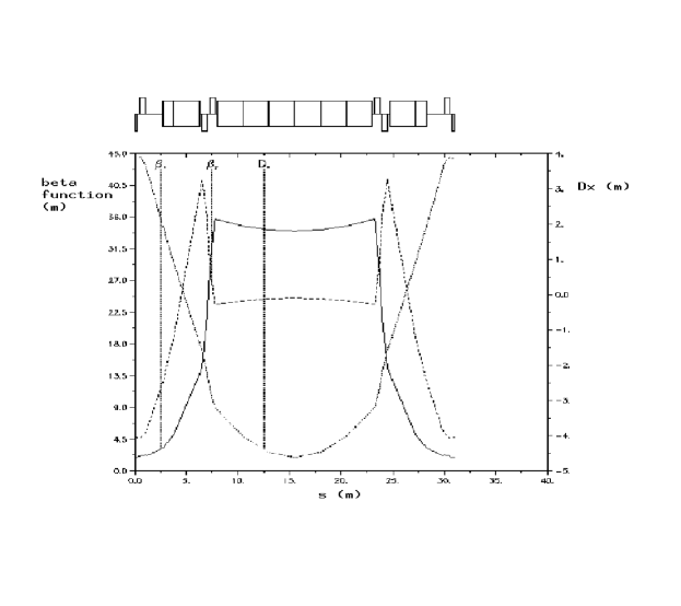

A very preliminary calculation of the dynamic aperture [190] without optimization of the lattice or inclusion of errors and end effects is given in Fig. 46. One would expect that simply turning off the chromatic correction sextupoles in the 4 cm mode would result in a linear lattice with a large transverse aperture. With only linear elements, the 4 cm optics was found to be strongly nonlinear with limited on-momentum dynamic acceptance.
A normal form analysis using COSY INFINITY [193] showed that the variation of tune shift with amplitude was large, which was the source of the strong nonlinearity in the seemingly linear lattice. To locate the source of this nonlinearity, a lattice consisting of the original IR and arcs only (no CC), was studied. Numerical studies confirmed similar dynamic aperture and variation of tune shift with amplitude. This ruled out the possibility that the dynamic aperture was limited by the low beta points in the local chromatic correction section and points to the IR as the source of the nonlinearity. These findings were also verified [194] using a Runge-Kutta integrator to track through the IR and a linear matrix for the rest of the lattice. Further analytical study using perturbation theory showed that the first order contribution to the tune shift with amplitude is proportional to and , which are large in this IR. These terms come from the nonlinear terms of and , which, to first order, equal the angular divergence of a particle. As a demonstration, a comparison to the LHC low beta IR was done. Taking into account only the drift from the IP to the first quadrupole, the horizontal detuning at 10 of the present IR ( 4 cm) is 0.01, whereas the detuning of the entire LHC lattice is below 1E-4. This also explains the fact that the on-momentum aperture of the wide momentum spread mode remains roughly constant despite various versions and correction attempts.
It was therefore concluded and later shown that the dynamic aperture of the more relaxed of 14 cm would not have the same strong nonlinearities due to the reduced angular terms. In fact, the variation of tune shift with amplitude was less by an order of magnitude; hence the large transverse acceptance shown in Fig. 46 (dashed line).
6 100 GeV CoM. Example (b)
The second lattice design, Example (b), is shown in Fig. 47 starting from the IP. The 1.5 m background clearing dipole is 2.5 m away from the IP and is followed by the triplet quadrupoles with the focusing quadrupole in the center. The interaction region (IR) stops at about 24 m from the IP. Because of the small low betatron functions in both transverse planes, the betatron functions at the final focusing triplets increase to m. The natural chromaticities, of order , are high, requiring local correction. Due to the size limitation of the collider ring, it appears that we have room for only two pairs of interleaved sextupoles on each side of the IP, each pair correcting chromaticity in one transverse plane. The correction section on each side of the IP spans a distance of roughly 61.3 m.

The SX1’s are the two horizontal correction sextupoles. They should be placed at positions with the same betatron functions and dispersion function, and separated horizontally and vertically by phase advances and so that their nonlinear effect will be confined in the region between the two sextupoles. Their horizontal phase advances should also be integral numbers of from the triplet focusing F-quadrupole so that the chromaticity compensation for that quadrupole will be most efficient [189]. The SX2’s are the two vertical correction sextupoles which should be placed similarly at designated locations. In general, it will be difficult to satisfy all the requirements mentioned; especially in this situation, luminosity arguments limit the lattice size. For this lattice, the Twiss properties at the centers of the four correction sextupoles are listed in table XII, where all the figures given by the lattice code are displayed. An attempt was made to satisfy all the requirements at the expense of having instead of 0.50 for the SX1’s. This trade-off is explained below.
| Distance | Phase Advances | Betatron Functions (m) | Dispersion | |||
|---|---|---|---|---|---|---|
| (m) | (m) | |||||
| SX2 | 33.5061 | 0.48826 | 0.74953 | 2.37647 | ||
| SX2 | 62.3942 | 0.98707 | 1.24953 | 2.37651 | ||
| SX1 | 49.3327 | 0.74892 | 0.87703 | 2.66039 | ||
| SX1 | 74.6074 | 1.24892 | 1.47987 | 2.65817 | ||
The second order effects of the sextupoles contribute to the amplitude dependent tune spreads, which, if too large, can encompass resonances leading to dynamical aperture limitation. For example, in this lattice,
| (28) | |||||
| (29) |
where and are the horizontal and vertical unnormalized emittances in m. In order to eliminate these tune spreads due to the sextupole nonlinearity, the sufficient conditions are [195]:
| (30) |
where for the th thin normal sextupole with strength ,
| (31) |
, and . The 5 requirements come about because there are 5 first order resonances driven by the sextupoles when the residual tunes of the ring satisfy , and two . The nominal tunes shown in Eq. (29) are far from these resonances. Therefore, the sines in the denominators of Eq. (30) can be omitted in this discussion. Since the strengths of SX1 and SX2 are similar, we have . In fact, they are roughly in the ratios of , which amount roughly to 1:10:100:1000 in this lattice. In above, represents either at the SX1’s or at the SX2’s, and represents either at the SX1’s or at the SX2’s. Thus, the first two restrictions in Eq. (30) are the most important, implying that all and for each pair of SX1’s must be made equal and between them must be strictly obeyed. The third restriction is the next important one, for which must be made equal for each pair of SX2’s and their horizontal phase difference must equal . The only two parameters left are between a pair of SX1’s and between a pair of SX2’s. They affect the restrictions for the resonances only, where the effective sextupole strengths and are involved. Thus if we allow one restriction to be relaxed, the relaxation of for the SX1’s will be least harmful.
Flexible momentum compaction (FMC) modules [192] are used in the arc. The momentum compaction of the arc has to be made negative in order to cancel the positive momentum compaction of the IR, so that the whole ring becomes quasi-isochronous. This is accomplished in three ways: 1) removing the central dipole of the usual FMC module; 2) increasing the length of the first and last dipoles, and 3) increasing the negative dispersion at the entrance. Two such modules will be required for half of the collider ring, one of which is shown in Fig. 48. To close the ring geometrically, there will be a m straight section between the two sets of FMC modules. The total length of the collider ring is now only m. This is a nice feature, since a small ring allows a larger number of collisions before the muons decay appreciably. Note that the IR and local correction sections take up 48.2% of the whole ring. The momentum compaction factor of this ring is now . The rf voltage required to maintain a bunch with rms length and rms momentum spread is , where is the slippage factor and the muon energy. On the other hand, if the bucket height is taken as times the rms momentum spread of the bunch, the rf harmonic is given by . Thus, for cm and , this lattice requires an rf voltage of kV. Since is negative already, its absolute value can be further lowered easily if needed. However, we must make sure that the contributions from the higher order momentum compaction are small in addition.

The dynamical aperture of the lattice is computed by tracking particles with the code COSY INFINITY [193]. Initially 16 particles with the same momentum offset and having vanishing and are placed uniformly on a circle in the - plane. The largest radius that provides survival of the 16 particles in 1000 turns is defined here as the dynamical aperture at this momentum offset and is plotted in solid in Fig. 49 in units of the rms radius of the beam. (At the 4 cm low beta IP, the beam has an rms radius of m.) As a reference, the 7 aperture spanning sigmas of momentum offset is also displayed as a semi-ellipse in dashdot. To maximize the aperture, first, the tunes must be chosen to avoid parametric resonances. The on-momentum amplitude dependent horizontal and vertical tunes are given in Eq. (29). With the designed rms m, the on-momentum tune variations are at most 0.0007. Second, the chromaticity variations with momentum must be as small as possible. This is shown in Fig. 49 (right hand side plot). Note that there are no families of sextupoles to correct for the higher order chromaticities in this small ring with only four FMC modules. As the momentum spread varies from to 0.9%, varies from 8.16698 to 8.07459, and from 6.28305 to 6.22369 for the center of the beam.
During aperture tracking we notice that particle loss occurs mostly in the horizontal direction. We are convinced that the small momentum aperture is a result of the large dispersion swing in the lattice from to m. For example, m dispersion and 0.6% momentum offset translates into a 2.7 cm off-axis motion. The nonlinearity of the lattice will therefore diminish the dynamical aperture. A resonant strength study using, for example, swamp plots and normalized-resonance-basis-coefficient analysis [196] actually reveals that this lattice and some of its variations are unusually nonlinear. Recently, we make a modification of the FMC arc modules which have a smaller dispersion swing from to m only. The IR has not been changed except for the matching to the arc modules. The aperture has been tracked with TEAPOT [197] in the same way as COSY and is plotted as dashes in Fig. 49 (left hand side plot). We see that the momentum aperture has widened appreciably. The dynamical aperture near on-momentum, however, is one sigma less than the lattice presented here. Nevertheless, it is not clear that this decrease is significant because all tracking has been performed in steps of one sigma only. However this type of aperture is still far from satisfactory, because so far we have been studying a bare lattice. The aperture will be reduced when fringe fields, field errors, and misalignment errors are included.
We suspect that the aperture for small momentum spread is limited by the dramatic changes in betatron functions near the IP [194]. These changes are so large that Hill’s equation would no longer be adequate and the exact equation for beam transport must be used. This equation brings in nonlinearity and limits the aperture, which can easily be demonstrated by turning off all the sextupoles. In other words, although the momentum aperture can be widened by suitable deployment of sextupoles, the on-momentum dynamical aperture is determined by the triplet quadrupoles and cannot be increased significantly by the sextupoles. Some drastic changes in the low beta design may be necessary.

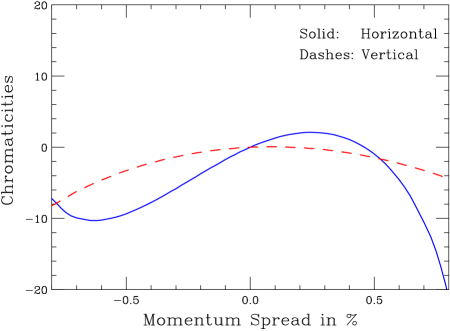
C Scraping
It has been shown [198] that detector backgrounds originating from beam halo can exceed those from decays in the vicinity of the interaction point (IP). Only with a dedicated beam cleaning system far enough from the IP can one mitigate this problem [188]. Muons injected with large momentum errors or betatron oscillations will be lost within the first few turns. After that, with active scraping, the beam halo generated through beam-gas scattering, resonances and beam-beam interactions at the IP reaches equilibrium and beam losses remain constant throughout the rest of the cycle.
Two beam cleaning schemes have been designed [188], one for muon colliders at high energies, and one for those at low energies.
The studies [188] showed that no absorber, ordinary or magnetized, will suffice for beam cleaning at 2 TeV; in fact, the disturbed muons are often lost in the IR, but a simple metal collimator was found to be satisfactory at 100 GeV.
1 Scraping for high energy collider
At high energies, a 3 m long electrostatic deflector (Fig. 50) separates muons with amplitudes larger than 3 and deflects them into a 3 m long Lambertson magnet, which extracts these downwards through a deflection of 17 mrad. A vertical septum magnet is used in the vertical scraping section instead of the Lambertson to keep the direction of extracted beam down. The shaving process lasts for the first few turns. To achieve practical distances and design apertures for the separator/Lambertson combinations, functions must reach a kilometer in the 2 TeV case, but only 100 m at 50 GeV. The complete system consists of a vertical scraping section and two horizontal ones for positive and negative momentum scraping (the design is symmetric about the center, so scraping is identical for both and ). The system provides the scraping power of a factor of 1000; that is, for every 1000 halo muons, one remains.
2 Scraping for low energy collider
At 50 GeV, collimating muon halos with a 5 m long steel absorber (Fig. 51) in a simple compact utility section does an excellent job. Muons lose a significant fraction of their energy in such an absorber (8% on average) and have broad angular and spatial distributions. Almost all of these muons are then lost in the first 50-100 m downstream of the absorber with only 0.07% of the scraped muons reaching the low quadrupoles in the IR, i.e. a scraping power is 1500 in this case, which is significantly better than with an earlier septum scraping system design [188] similar to that developed for the high energy collider.
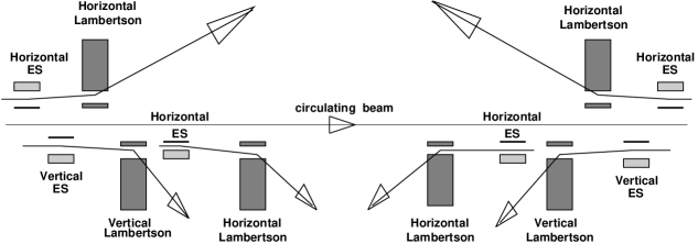
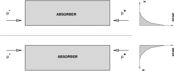
D Beam-beam tune shift
Several studies have considered beam emittance growth due to the beam-beam tune shift and none have observed significant luminosity loss. For instance, a study [199], using the high energy collider parameters (see table I), in which particles were tracked assuming Gaussian beam field distributions, and no muon decay, showed a luminosity loss of only 4%. With muon decay included, the loss contribution from beam-beam effects is even less. Another study [200] using a particle in cell approach with no assumptions about field symmetry obtained a similar result. Collisions between beams displaced by 10% of their radius also gave little loss. But all these studies assumed an ideal lattice, and none considered whether small losses due to nonlinearities give rise to an unacceptable background.
E Impedance/wakefield considerations
A study [201] has examined the resistive wall impedance longitudinal instabilities in rings at several energies. At the higher energies and larger momentum spreads, solutions were found with small but finite momentum compaction and moderate rf voltages. For the special case of the Higgs Factory, with its very low momentum spread, a solution was found with no synchrotron motion, but rf was provided to correct the first order impedance generated momentum spread. The remaining off-momentum tails which might generate background could be removed by a higher harmonic rf correction without affecting luminosity. Solutions to the higher energy and larger momentum spread cases without synchrotron motion are also being considered.
Given the very slow or nonexistent synchrotron oscillations, the transverse beam breakup instability is significant. This instability can be stabilized using rf quadrupole [181] induced BNS damping. For instance, the required tune shift with position in the bunch, calculated using the two particle model approximation [202], is only for the 3 TeV case using a 1 cm radius aluminum pipe. This stabilizes the resistive wall instability. However, this application of BNS damping to a quasi-isochronous ring, and other head-tail instabilities due to the chromaticities and , needs more study.
F Bending magnet design
The dipole field assumed in the 100 GeV collider lattices described above was 8 T. This field can be obtained using niobium titanium (NbTi) cos theta superconducting magnets similar to those developed for the LHC. The only complication is the n eed for a tungsten shield between the beam and coils to shield the latter from beam decay heating.
The ’s decay within the rings (), producing electrons whose mean energy is approximately that of the muons. With no shielding, the average power deposited per unit length would be about 2 kW/m in the 4 TeV machine, and 300 W/m in the 100 GeV Higgs factory. Figure 52 shows the power penetrating tungsten shields of different thickness [44, 187, 188, 203]. One sees that 3 cm in the low energy case, or 6 cm at high energy would reduce the power to below 10 W/m, which can reasonably be taken by superconducting magnets.
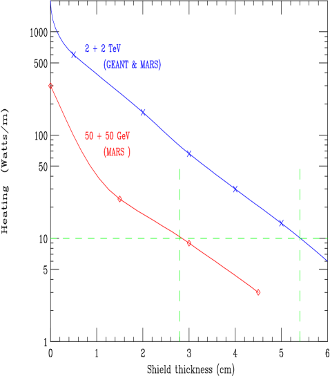
Figure 53 shows the cross section of a baseline magnet suitable for the 100 GeV collider.
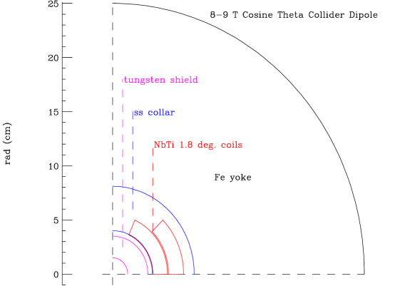
The quadrupoles could use warm iron poles placed as close to the beam as practical. The coils could then be either superconducting or warm, placed at a greater distance from the beam and shielded from it by the poles.
The collider ring could be made smaller, and the luminosity increased, if higher field dipoles were used. In the low energy case, the gain would not be great since less than half the circumference is devoted to the arcs. For this reason, and to avoid yet another technical challenge, higher field magnets are not part of the baseline design of a 100 GeV collider. But they would give a significant luminosity improvement for the higher energy colliders, and would be desirable there. There have been several studies of possible designs, three of which (two that are promising and one that appears not to work) are included below.
1 Alternative racetrack Nb3Sn dipole
A higher field magnet based on Nb3Sn conductor and racetrack coils is presently being designed. The Nb3Sn conductor allows higher fields and provides a large temperature margin over the operating temperature, but being brittle and sensitive to bending or other stress, presents a number of engineering challenges.
In this design, the stress levels in the conductor are reduced by the use of a rectangular coil block geometry and end support problems are reduced by keeping the coils flat. In the more conventional cos theta designs, the conductor is distributed around a cylinder and the forces add up towards the midplane; in addition, the ends, as they arc over the cylinder, are relatively hard to support.
The geometry of the cross section is shown in Fig. 54. It uses all 2-D flat racetrack coils. Each quadrant of the magnet aperture has two blocks of conductors. The block at the pole in the first quadrant has a return block in the second quadrant, similar to that in a conventional design. The height of this block is such that it completely clears the bore. In a conventional design, the second block, the midplane block, would also have a return block in the second quadrant. That would, however, require the conductor block to be lifted up in the ends to clear the bore and thus would lose the simple 2-D geometry. In the proposed design, the return block retains the 2-D coil geometry, as it is returned on the same side (see Fig. 54) and naturally clears the bore. Since the return block does not contribute to the field, this design uses 50% more conductor. This, however, is a small penalty to pay for a few magnets where the performance and not the cost is a major issue. The field lines are also shown in Fig. 54.
Preliminary design parameters for two cases are given in table XIII. The first case is one where the performance of the cable used is the same that is in the LBL D20 magnet, which created a central field of 13.5 T. The second case is the one where the cable is graded and two types of cable are used, and it is assumed that a reported improvement in cable performance is realized. It is expected to produce a central field of 14.7 T when operated at K.
| Case 1: Same conductor as in LBL 13.5 T D20 magnet without grading | |
|---|---|
| Central field at quench | 13 T at |
| Coil dimensions | mm |
| Total number of racetrack coils in whole magnet | 6 |
| Total number of blocks per quadrant in aperture | 2 (+1 outside the aperture) |
| Yoke outer radius | 500 mm (same as in D20) |
| Field harmonics | a few parts in at 10 mm |
| Midplane gap (midplane to coil) | 5 mm (coil to coil 10 mm) |
| Minimum coil height in the end | 45 mm (Note: coils are not lifted up.) |
| Case 2: Newer conductor and graded | |
| Central field at quench | 14.7 T at |
| Grading | 70 mm divided in two 35 mm layers |
| Overall current densities | 370 A/mm2 and 600 A/mm2 |
| Peak fields | 16 T and 12.5 T |
| Copper current density | 1500 A/mm2 |
| Other features are the same as in Case 1 | |
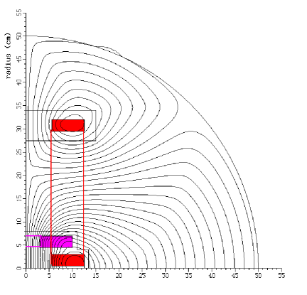
2 Alternative Cos Theta Nb3Sn dipole
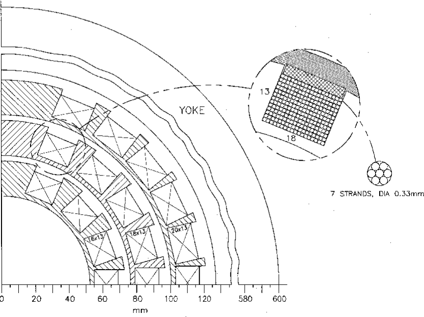
In this case the problem with the brittle and sensitive conductor is solved by winding the coil inside many separate slots cut in metal support cylinders. There is no build up of forces on the coil at the mid-plane. The slots continue around the ends, and thus solve the support problem there too.
Figure 55 shows this alternative Nb3Sn dipole cos theta design. It is an extension of the concept used to build helical magnets [204] for the polarized proton program at RHIC [205]. The magnet is wound with pre-reacted, kapton-insulated, B-stage impregnated, low current cable. The build up of forces is controlled by laying the cables in machined slots in a metal support cylinder. After winding, the openings of the slots are bridged by metal spacers and the coils pre-compressed inward by winding B-stage impregnated high tensile thread around the spacers. After curing, the outside of each coil assembly is machined prior to its insertion into an outer coil, or into the yoke. There are 3 layers. The inner bore is 55 mm radius, the outer coil radius approximately 118 mm, and the yoke inside radius is 127 mm. The maximum copper current density is 1300 A/mm2.
Using the same material specifications as used in the above high field option, a central short sample field of 13.2 T was calculated. This is somewhat less than the block design discussed above, but could be improved by increasing the cable diameters to improve the currently rather poor (64%) cable to cable-plus-insulator ratio.
3 Study of C-magnet dipole
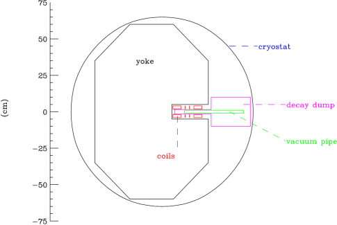
Figure 56 shows the cross section of a high field dipole magnet in which it was hoped to bring the coils closer to the beam pipe without suffering excessive heating from beam decay. The coil design [206] appeared reasonable, but the required avoidance of coil heating was not achieved.
Decay electrons are generated at very small angles () to the beam, and with an average energy about 1/3 of the beam. Such electrons initially spiral inward (to the right in Fig. 56) bent by the high dipole field. In the high energy case, these electrons also radiate a significant fraction of their energy as ( 1 GeV) synchrotron gamma rays, some of which end up on the outside (to the left in Fig. 56). The concept was to use a very wide beam pipe, allow the electrons to exit between the coils, and be absorbed in an external cooled dump. Unfortunately a preliminary study found that a substantial fraction of the electrons did not reach the dump. They were bent back outward before reaching it by the return field of the magnet coils and the nature of the curved ring geometry. Such electrons were then trapped about the null in the vertical field and eventually hit the upper or lower face of the unshielded vacuum pipe. They showered, and deposited unacceptable levels of heat in the coils.
Another idea called for collimators between each bending magnet that would catch such trapped electrons. This option has not been studied in detail, but the impedance consequences of such periodic collimators are expected to be unacceptable.
Further study of such options might find a solution, but the use of a thick cylindrical heavy metal shield appears practical, adequate, and is thus the current baseline choice.
G Energy scale calibration
In order to scan the width of a Higgs boson of mass around 100 GeV, one needs to measure the energy of the individual muon stores to an accuracy of a few parts per million, since the width of a Higgs boson of that mass is expected to be a few MeV. Assuming that muon bunches can be produced with modest polarizations of and that the polarization can be maintained from turn to turn in the collider, it is possible to use the precession of the polarization in the ring to measure accurately the average energy of the muons [12]. The total energy of electrons produced by muon decay observed in the calorimeter placed in the ring varies from turn to turn due to the precession of the muon spin, which is proportional to the Lorentz factor of the muon beam. Figure 57 shows the result of a fit of the total electron energy observed in a calorimeter to a functional form that includes muon decay and spin precession. Figure 58 shows the fractional error obtained from a series of such fits plotted against the fractional error of measurement in the total electron energy that depends on the electron statistics. It has been shown that precisions of a few parts per million in are possible with modest electron statistics of detected. It should be noted that there are decays per meter for a muon intensity of muons.


Our current plans to measure the energy due to decay electrons entail an electromagnetic calorimeter that is segmented both longitudinally and transversely and placed inside an enlarged beam pipe in one of the straight sections in the collider ring. The length of the straight section upstream of the calorimeter can be chosen to control the total number of decays and hence the rate of energy deposition. The sensitive material can be gaseous, since the energy resolution is controlled by decay fluctuations rather than sampling error. In order to measure the total number of electrons entering the calorimeter, we plan to include a calorimeter layer with little absorber upstream of it as the first layer.
This scheme will enable us to calibrate and correct the energy of individual bunches of muons and permit us to measure the width of a low mass Higgs boson.
VIII RADIATION AND BACKGROUNDS
A Conventional radiation
The proton source generates a 4 MW proton beam, which is comparable to the proposed spallation source [92]. This is a very high power and will, as in the spallation source, require great care in reducing unwanted particle losses, as well as careful machine shielding, and target and beam dump design. Initial studies of the target and capture solenoid region have been performed with the MARS code, and preliminary specifications for shielding determined, but more work is needed.
The cooling and accelerator chain is rather clean, since a relatively small fraction of the muons decay, and their energies are low. Power deposited in the accelerators is typically 10-30 W/m (see table IX and table X).
If no muons are lost, then the only sources of radiation are the muon decays yielding electrons and neutrinos. The neutrino radiation we discuss below. The electrons shower in the collider beam pipe shields, depositing most of their energy there and a relatively small amount in the magnet coils and yoke. Radioactivation levels, as calculated by MARS [207], after five years of 4 TeV collider operation are given in table XIV for the cases immediately after turn off and 1 day after turn off. It is seen that the areas in the tunnel that are outside the magnets are relatively free of radioactivation. Special procedures will be needed when the shield pipe has to be opened, as for instance when a magnet is changed. For the lower energy colliders, the radioactivation levels are proportionally less.
| immediate | after 1 day | |
|---|---|---|
| Inside face of shield | 9000 | 4000 |
| Outside face of shield | 200 | 170 |
| Outside of coils | 30 | 14 |
| Outside of yoke | 3 | 1.4 |
If muons are lost either accidentally, by scraping, or deliberately after some number of turns, then the muons penetrate to considerable distances in the soil/rock (3.5 km at 2 TeV, 800 m at 250 GeV) and deposit their energy directly or through their interaction products. Figure 59 and Fig. 60 show the distribution of radiation levels, assuming 25% of all muons (4 bunches of at 15 Hz) are dumped into soil/rock with density 2.24 g/cm3. The outer contours correspond to the federal limits, reaching at maxima of 18 m (2 TeV) and 14.5 m (250 GeV). To confine this radiation beneath the ground one can deflect the extracted beams down by 4.5 mrad at 2 TeV and about 10 mrad at 250 GeV. If any water were present in the soil/rock, then the first two meters around the tunnel and around the aborted beam axis would require insulation or drainage up to a distance of 2.5 km at 2 TeV or 550 m at 250 GeV.
B Neutrino induced radiation
It has been shown [64, 208, 209, 210, 211] that the neutrinos created in muon beam decays can generate excessive secondary radiation at large distances from a muon collider (see Fig. 61). The surface radiation dose in units of equivalent [212] doses () over a time , in the plane of a bending magnet of field B(T), in a circular collider with beam energy , average bending field , at a depth (assuming a spherical earth), with muon current (of each sign) of is given by:
| (32) |
and the dose at a location on the surface, in line with a high beta straight section of length is:
| (33) |
The equation for assumes that the average divergence angles satisfy the condition: . This condition is not satisfied in the straight sections approaching the IP, and these regions, despite their length, do not contribute a significant dose.
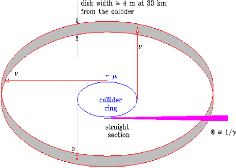
For the 3 TeV parameters given in table I and muon currents and m, and taking the Federal limit on off-site radiation dose/year, to be 1 mSv/year (100 mrem/year), the annual dose (1 year is defined as s), in the plane of a bending dipole is,
| (34) |
and for a straight section of length 0.6 m is:
| (35) |
which may be taken to be within a reasonable limit. The general trend of these expressions has been verified by Monte Carlo simulations [213] using MARS. In particular, for the 3 TeV case the needed depth to stay within is 300 m instead of 500 m.
Special care will be required in the lattice design to assure that no field- free region longer than 0.6 m is present. This may sound difficult, but it may be noted that the presence of a field of even 1 T, is enough to reduce the dose to a level below the Federal limit. The application of such a field over all rf and other components seems possible [213].
For lower energy machines, the requirements rapidly get easier: a 0.5 TeV machine at 100 m depth could have 25 m long sections, for the same surface dose. For a 100 GeV machine the doses are negligible.
For machines above 3 TeV, various strategies can be employed:
-
The machines could be built at greater depths (mines many km deep are common).
-
The vertical beam orbits in the machine could be varied so as to spread the plane of radiation and thus reduce the peak doses.
-
The specific locations in line with straight sections could be purchased and restricted.
-
Straight sections could be shortened further by using continuous combined function magnets.
-
The machines could be built on an island, but this could have difficulties associated with access to power and other utilities.
But for any large increase in energy, to 10 TeV for instance, some reduction in muon beam flux probably will be required. The resultant loss of luminosity might be made up in a number of ways [4]:
-
The beam-beam tune shift constraint could be avoided by introducing a conducting medium (e.g. liquid lithium) at the interaction point [214].
-
The focusing strength could be increased by the use of plasma or other exotic focusing method.
-
Better cooling could be developed. Optical stochastic cooling [137], for instance, might reduce the emittances by many orders of magnitude, thus greatly reducing the required beam currents. Indeed, such cooling would require lower currents to function appropriately.
Such options will need future study.
C Muon decay background
With muons per bunch in a TeV collider ring there are approximately muon decays per meter giving rise to high energy electrons. These off-energy, off-axis electrons undergo bremsstrahlung when they traverse magnetic fields. When they exit the beam pipe they interact and produce electromagnetic showers and, to a lesser extent, hadrons and muons. Much of this debris can be locally shielded, so the primary concern is muon decays near the interaction point [44]. This is the background we discuss in some detail below.
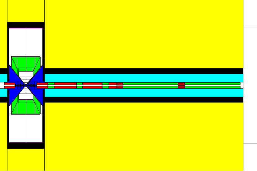
Detailed Monte Carlo simulations of electromagnetic, hadronic and muon components of the background [44, 187, 198, 203, 213, 215, 216] have been performed using the MARS [115] and GEANT [148] codes. The most recent study [215] has been done with GEANT. Figure 62 shows the final 130 meters of the 2 + 2 TeV detector region in this study. It includes the final four quadrupoles, dipoles and a solenoidal field surrounding the detector. This study:
-
followed shower neutrons and photons down to keV and electrons to keV.
-
used a tungsten shield over the beam, extending outward to an angle of 20 degrees from the axis.
-
Inside this shield, the clear radius has a minimum, in the high energy cases, at a distance from the IP of 1.1 m (80 cm for 50+50 GeV). At this point, and in an expanding cone beyond it, the clear radius is maintained at approximately 4 sigma of the beam size.
-
Between this minimum aperture point and the IP, the clear radius follows an inverse cone, increasing as it approaches the IP, with an angle a little greater than the 4 sigma of the beam divergence. These cones are designed so that the detector could not ‘see’ any surface directly illuminated by the initial decay electrons, whether in the forward or backward (albedo) direction (see figure 63).
-
The resulting open space between the IP and the tip of the cone is approximately 3 cm in the 4 TeV and 500 GeV CoM cases, and approximately 6 cm in the 100 GeV CoM case.
-
The inner surface of each shield is shaped into a series of collimating steps and slopes to maximize the absorption of electron showers from electrons at very small angles to the cone surface, thus reducing the funnelling of low energy electrons down the pipes.
-
Further upstream, prior to the first quadrupole (from 2.5 to 4 m in the Higgs case), an 8 T dipole, with collimators inside, is used to sweep decay electrons before the final collimation.
Note that there is currently an inconsistency, in the very low Higgs Factory Case, between the short open space between shields (+/- 6 cm) and the rms source length () of 10 cm. Some modifications to the parameters and shielding design will be required for this case.
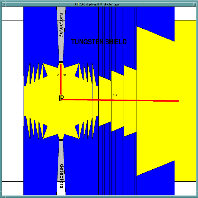
Every modern detector will have to be able to identify and reconstruct secondary vertices such as those associated with b-quark decays. In order to estimate the viability of a vertex detector we have to show that the occupancy of its elements is not higher than about Figure 64 shows the occupancy as a function of radial distance from the interaction point for the three CoM energies studied : 0.1, 0.5 and 4 TeV. The occupancy was calculated for silicon pads of , and assuming interaction probabilities of 0.003 and 0.0003 for low energy photons and neutrons respectively. One can observe that the total occupancy (left figure) is above one percent for small radii. Most of the hits is due to conversions of photons. The occupancy due to hits resulting from charged particles is below (right hand figure). One can lower the occupancy at small radii by using smaller pixel sizes, as indicated in table XV below, as well as by using innovative detector ideas as described in the next section.
Table XV gives the hit density for the Higgs factory from the various sources and the occupancy of pixels of the given sizes; in each case the number is given per bunch crossing. The hit density for the higher energy machines is found to be somewhat lower due to the smaller decay angles of the electrons.
| Radius | 5 | 10 | 20 | 100 | |
|---|---|---|---|---|---|
| Photons hits | 26 | 6.6 | 1.6 | 0.06 | |
| Neutrons hits | 0.06 | 0.08 | 0.2 | 0.04 | |
| Charged hits | 8 | 1.2 | 0.2 | 0.01 | |
| Total hits | 34 | 8 | 2 | 0.12 | |
| Pixel size | |||||
| Total occupancy | % | 0.6 | 0.14 | 0.4 | 0.02 |
| Occupancy charged | % | 0.14 | 0.02 | 0.04 | 0.002 |
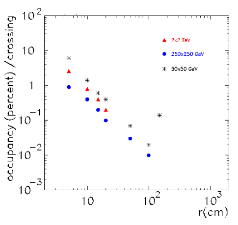
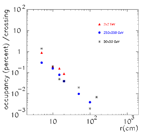
The radiation damage by the neutrons on a silicon detector has also been estimated. In the Higgs case, at 5 cm from the vertex, the number of hits from neutrons above 100 keV is found to be per year. This is significantly less than that expected at the LHC which is now ordering silicon detectors claimed to survive hits, approximately three times that assumed here. The damage for silicon detectors in the higher energy machines is of the same order (see table XVI).
| CoM | ’s/bunch | neutrons/cm2/crossing | Hits/year | Lifetime |
|---|---|---|---|---|
| (TeV) | (above 100 KeV) | (years) | ||
| 4 | 2 | 100 | 3 | 5 |
| 0.5 | 4 | 50 | 3 | 5 |
| 0.1 | 4 | 30 | 1.8 | 8 |
D Halo background
Muon halo refers to those muons which are lost from the beam bunch as it circulates around the collider ring. In conventional electron or proton accelerators, beam particles which are lost away from the IP are of little concern as they can be locally shielded. However, muons can traverse long distances and therefore have the potential to generate background in a detector. The magnitude of this background depends on a detailed knowledge of the injected beam profile and a credible model for beam halo and beam losses. More work is needed before these are well enough understood. Nevertheless, it is clear that the beam will need careful preparation before injection into the collider, and the injection system will have to be precise and free of ripple.
The collimation system described in the previous subsection was designed to scrape the beam both initially and during the 1000 turns, to assure that all loss occurs at the scraper and not near the IP. That study indicated suppressions better than 103 of background in the detector [188].
Beam loss must be limited as far as possible. Gas scattering has been studied [217] and shown to give a negligible contribution. The effects of beam-beam scattering are under study and need further work. Momentum spread tails from uncorrected wakefield effects must be controlled. Assuming that the total loss from all causes, after injection and the first few turns is less than in 1000 turns, (i.e. per turn), then the number of background muons passing through the detector should be less than 800 () per turn. This is a low density of tracks per cm2 and should be acceptable, but lower losses or better scraping would be desirable.
E Pair production
Coherent beam-beam electron pair production (beamstrahlung) has been shown [200, 218] to be negligible, but the incoherent pair production (i.e. ) in the 4 TeV collider case is significant.
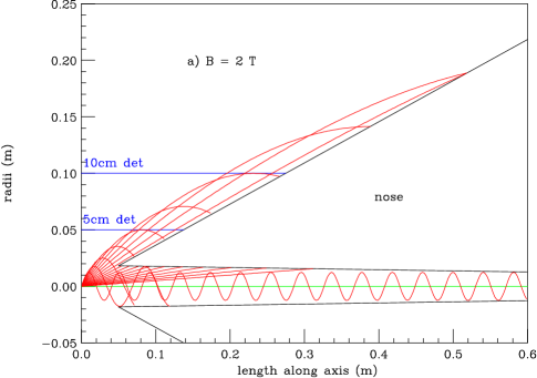
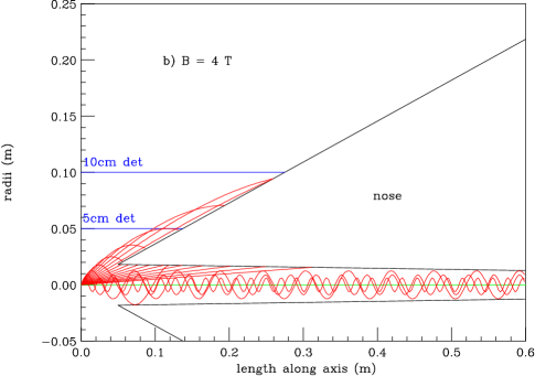
The cross section is estimated to be mb [218], which would give rise to a background of electron pairs per bunch crossing. The electrons at production do not have significant transverse momentum but the fields of the on-coming m bunch can deflect them towards the detector. A simple program was written to track electrons from close to the axis (the worst case) as they are deflected away from the bunch center. Once clear of the opposing bunch the tracks spiral under the influence of the experimental solenoid field. Figures 65 shows the radii vs. length of these electron tracks for initial momenta from 3.8 to 3000 MeV in geometric steps of Fig. 65(a) is for a solenoidal field of 2 T and Fig. 65(b) for 4 T. In the 2 T case tracks with initial energy below 30 MeV do not make it out to a detector at 10 cm, while those above 100 MeV have too small an initial angle and remain within the shield. Approximately 10% (3000 tracks) of these are in this energy range and pass through a detector at 10 cm. The track fluences at the ends of the detector are less than 10 tracks per cm2 which should not present a serious problem. At 5 cm, there are 4500 tracks giving a fluence of 30 per cm2, which is also probably acceptable. If the detector solenoid field is raised to 4 T, then no electrons reach 10 cm and the flux at 5 cm is reduced by a factor of 2.
F Bethe-Heitler muons
| CoM Collider Energy (TeV) | 4 | 0.5 | 0.1 |
| Assumed source length (m) | 130 | 33 | 20 |
| per electron | |||
| Beam ’s per bunch | |||
| Bethe-Heitler ’s per bunch crossing () | 28 | 17.5 | 6.1 |
| initial (GeV) | 22 | 9.5 | 4.4 |
| ’s entering calorimeter | 220 | 160 | 25 |
| (GeV) | 15.4 | 6.3 | 1.8 |
| (GeV) | 2.9 | 1.3 | 0.4 |
| Total (GeV) | 640 | 210 | 10 |
| pedestal subtracted (GeV) | 50 | 25 | 1 |
| Fluctuation in (GeV) | 55 | 15 | 1 |
| pedestal subtracted (GeV) | 15 | 15 | .5 |
| Fluctuation in (GeV) | 40 | 8 | 0.5 |
The GEANT/MARS studies [44, 203, 207] also found a significant flux of muons with quite high energies, from pair production in electromagnetic showers (Bethe-Heitler). Figures 66 and 67 show the trajectories of typical muons from their sources in the shielding around the beam pipe to the detector. Figure 66 is for a 4 TeV CoM collider, where the muons have high energy and long path lengths. A relatively long (130 m) section of beam pipe prior to the detector is shown. Figure 67 is for the 100 GeV CoM collider for which, since the muons have rather short path lengths, only a limited length of beam pipe is shown. Note that the scales are extremely distorted: the 20o shielding cones on the right hand of the figures appear at steeper angles.
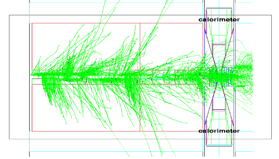
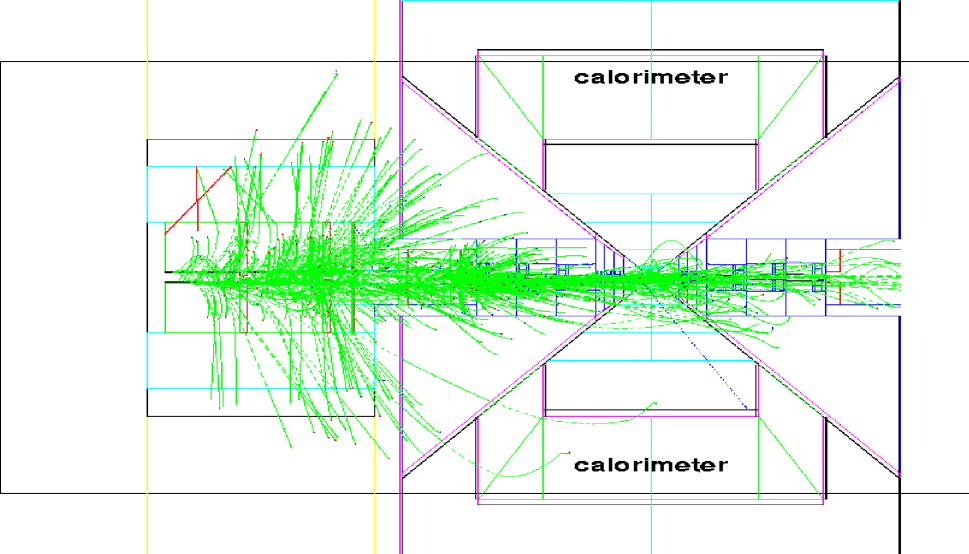
The most serious effect appears to arise when these muons make deeply inelastic interactions and deposit spikes of energy in the electromagnetic and hadronic calorimeters. This is not serious in the Higgs case, for which the fluxes and cross sections are low, but at the higher collider energies they generate significant fluctuations in global parameters, such as transverse energy and missing transverse energy.
Table XVII gives some parameters of the muons for three different machine energies. In the 4 TeV and 500 GeV CoM cases, massive lead shielding outside the focus quadrupoles has been included.
Figures 68 and 69 show energy deposition from Bethe-Heitler muons in a typical bunch crossing. These depositions are plotted against the cosine of the polar angle and azimuthal angle in the calorimeter for 4 TeV and for 500 GeV CoM, respectively. The massive lead shielding referred to above was not included in this study. Right hand plots in Figs. 68 and 69 show the same distributions with a 1 ns timing cut. It is seen that the timing cut, if it is possible, is effective in removing energy spikes at small rapidity, but has little effect in the forward and backward directions. The overall reduction in energy deposition is about a factor of two.
The energy spikes can cause at least three problems: 1) they affect the triggers and event selections based on overall or transverse energy balance; 2) they can generate false jets and 3) they can give errors in the energies of real jets. After a pedestal subtraction, the effects on energy balances do not seem serious. The generation of false jets can be eliminated by a longitudinal energy distribution cut without introducing significant inefficiency. Energy errors in real jets appear to be the most serious problem. They can be reduced by the application of radial energy distribution cuts, but such cuts introduce significant inefficiencies for lower energy jets. More study is needed.
Earlier studies [216] with MARS, using less sophisticated shielding, gave results qualitatively in agreement with those from GEANT.


IX DETECTOR SCENARIOS
The background consists of neutral and charged particles. For neutrons, the longitudinal and radial fluences were found to be comparable. The photons (average energy about 1 MeV) show a clear radial source. The charged particles and the photons do not all point back to the interaction point, but to the general vicinity of the IP, namely to the region where the 20 degree tungsten shield becomes thinner. The flux of secondary muons (Bethe-Heitler pairs) is mainly longitudinal.
We would expect this background to pepper the tracking volume with random hits and produce significant energy pedestals in the calorimeter cells. These effects are considered in more detail in the following sections. In general, in designing a strawman detector that must operate in a large background flux we will want to employ as many detector channels as is practical. A strawman muon collider detector design with a few times non-pixel channels would seem reasonable [219]. Over the last few years, development of pixel detectors has resulted in a quantum jump in the number of electronic channels. For example, the SLD vertex detector [220] contains pixels, and similar numbers of pixels are planned for the LHC vertex detectors. Hence, a strawman muon collider vertex detector employing pixels would seem reasonable.
A Silicon vertex detector schemes
From table XVI, it can be seen that the radiation damage to silicon detectors is acceptable in terms of the number of hits per year and the resultant lifetime of the detector. This prompts [219] us to consider the following options for silicon vertex detector design for the muon collider:
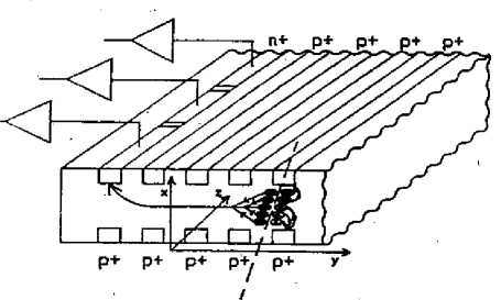

-
Silicon drift detector. The idea, which is described in the muon collider feasibility study [44, 33], is to exploit the time gap between bunch crossings by using the silicon drift detector technology [221] (see Fig. 70). Using m2 detectors it should be possible to obtain a resolution of a few microns in the drift direction. This would facilitate a very precise vertex detector, although questions of radiation hardness remain to be resolved for this option.
-
Columnar pixels [222]. The idea is to exploit the very well localized primary vertex position by using long thin tracking pixels that point at the IP and therefore record large ionization signals only for tracks coming from the IP (Fig. 71). For example, one can construct m2 pixels that are 300 m deep. The pixels are produced using controlled feed-through-drilling technology to create a lattice of anodes and cathodes that extend through the 300 m thick wafer.
-
Pixel micro-telescopes [223]. The idea is to replace a single pixel layer with two layers separated by a small distance, and read them out by taking the AND between appropriate pairs. The distance between the layers is optimized so that soft MeV tracks (which are associated with almost 80% of the predicted background hits) produced in one layer curl up in the magnetic field before reaching the second layer. Thus, the pixel micro-telescope is blind to the soft background hits and also blind to tracks that do not come from the IP. In the example shown in Fig. 72 the top measurement layer has a finer granularity than the bottom confirmation layer. The corresponding rows in the two pixel layers can be read out with different clock speeds to maintain the correct correspondence at the input into the AND gate that registers valid hits in the telescope. If the readout rows are the ones parallel to the beam direction, then variable clock speeds can be used to maintain the correct accepted direction with respect to the IP.
The challenge of a high background environment is clearly fruitful ground for new ideas. The above considerations suggest that, provided silicon detectors can be used in the inner tracking volume, it should be possible to construct a vertex detector able to tag secondary vertices from short lived particles at a muon collider. Detailed simulations are currently underway to establish this more concretely.
B Outer tracking schemes
The predicted background fluxes for a Higgs factory detector at a radius of 50 cm are 200 photons/cm 350 neutrons/cm and 0.08 charged tracks per cm The neutron flux is therefore about the same as the flux in the inner tracking volume, whereas the photon and charged particle fluxes are significantly less than those predicted at smaller radii. There are two alternative tracking strategies under consideration:
-
Low field, large tracking volume drift chamber option. This option, which is described in the muon collider book [224], uses a TPC to exploit the 20 s time between bunch crossings. This option is viable for the very high energy muon collider ( TeV). The large neutron flux necessitates choosing a gas that does not contain hydrogen. A mixture of 90% neon plus 10% CF4 gives a drift velocity of 9.4 cm/s, which is close to that required to match the bunch crossing time. High- tracks from the IP embedded in the predicted background flux have been simulated for the TPC shown in Fig. 73. The simulation includes ionization, drift and diffusion of the electrons in the gas, multiplication, and other details of the detection process. The majority of the background hits arises from low energy Compton recoils yielding very low energy electrons that have a radius of curvature of less than 1 mm in the 2 T field. Their projection on the readout plane covers not more than one readout pitch (0.3 0.4 cm2). These background electrons, together with the nuclear recoils from neutron scatters, yield large pulses that can be removed by cutting on the maximum acceptable pulse height. The simulation predicts that with an average background flux of 100 photons/cm2, reasonable pulse height cuts remove only 1% of the effective TPC volume, and yield tracks of high quality. However, it was realized that positive ion build-up may be a problem with the design shown in Fig. 73. If this problem can be overcome, the design shown in the figure yields a simulated momentum resolution of about 1.2% for tracks with p GeV/
-
High field, compact silicon tracker option. An alternative strategy is to make a compact tracker by using silicon in a high field (for example, 4 T).
FIG. 74.: Compact tracker geometry in a 4 T field. As an example, consider the geometry shown in Fig. 74 in which a 4-layer pixel vertex detector is embedded in a 4-layer small angle stereo cylindrical silicon microstrip detector with a m2 resolution. We take the inner layer of the vertex detector to consist of a cylinder of m2 pixels, and the outer 3 vertex layers to consist of spherical shells of m2 columnar pixels or pixel micro-telescopes. The system is assumed to correspond to 15% of a radiation length at . Using a parametric calculation of the momentum resolution, including multiple scattering, we obtain (GeV/ for p = 100 GeV/ (1 GeV/
Both the low field and high field tracking solutions look interesting and should be pursued with more complete simulations.
C Electromagnetic calorimeter schemes
Background particles entering the electromagnetic calorimeter are expected to give rise to significant energy pedestals in the calorimeter cells. Consider a 4 m long calorimeter that is 25 radiation lengths deep, has an inner radius of 120 cm, and is constructed from cm2 cells. This gives a total of electromagnetic calorimeter towers. The GEANT background calculation predicts that each cell sees on average background photons per crossing with a mean energy MeV. If an electromagnetic shower occupies 9 cells, then the mean background pedestal will be about 70 MeV. This pedestal can be subtracted from the measured energies. The precision of the resulting electron and photon energy measurements will depend on the fluctuations in the mean background energy per cell. For an electromagnetic shower occupying 9 cells, the fluctuations in the pedestals are predicted to be about 10 MeV. This takes into account the fluctuations in the number and the energies of the background photons.
D Hadronic calorimeter schemes
None of the energy generated by background photons in the electromagnetic calorimeter is expected to penetrate into the hadronic calorimeter. GEANT calculations show that the total kinetic energy deposited by neutrons in the calorimeter is of the order of 140 TeV with an average energy of 30 MeV per neutron. In order to estimate what fraction of the kinetic energy of the neutrons will be visible, we should consider the materials involved. For this simulation we have presumed an equal mix by volume of liquid argon (as active medium) and copper (as absorber). At 30 MeV we expect only a small fraction of the neutrons to knock off protons and only about 10% of the proton ionization to be visible in the liquid. Presuming a hadronic calorimeter with towers, with the material composition described above, the average energy read in the liquid argon will be of the order of 10 MeV per tower with a fluctuation of 5 MeV. In summary, a GeV collider with muons per bunch, the photons and neutrons are expected to generate pedestals of 800 and 100 GeV respectively. The estimates for pedestal fluctuations are at or below the level of the expected electronic noise. Therefore we believe that the subtraction of these pedestals would present little problem both for the electromagnetic and the hadronic calorimeters. The presence of the high neutron background should be taken into account in choosing materials for calorimetry. Liquid argon seems a natural choice for the electromagnetic calorimeter.
The energy deposited by the Bethe-Heitler muons in the calorimeter is given in table XVII as a function of the center of mass energy of the collider. For low center of mass energies, such as the Higgs factory, the Bethe-Heitler muons are not a problem, since there are fewer of them and they leave less energy by catastrophic bremsstrahlung in the calorimeter. For the higher energy option (4 TeV in the CoM or higher), one should explore ways to correct for the energy deposition in the calorimeter, such as pattern recognition of the muon tracks or by using timing information.
E Muon detector schemes
The predicted background flux is expected to be relatively modest beyond a radius of 3 m in the vicinity of the muon detector. Several possible technologies for muon detectors at a muon collider were discussed during Snowmass[33]:
-
Cathode strip chambers. The idea, which is described in the muon collider book [224], is to use MWPCs with segmented cathodes and a short (35 ns) drift time to provide prompt signals for triggering. The precision of the coordinate measurements would be expected to be of order 50 m a few mm.
-
Threshold Cherenkov counter. The idea is to use a gas Cherenkov radiator to exploit the directionality of Cherenkov radiation in order to select high- muons coming from the IP. The device would also give excellent timing resolution (of order 2 ns).
-
Long drift jet chamber with pad readout [225] (Fig. 75). Drift time provides the z coordinate, and pad readout provides the r- coordinates. Directionality at the trigger level is provided by the pattern of pad hits within a limited time window. The drift field is provided by cathode strips on grooved G-10 plates. Using 90% argon plus 10% CF4 and a maximum drift distance of 50 cm, the maximum drift time is 5 s.
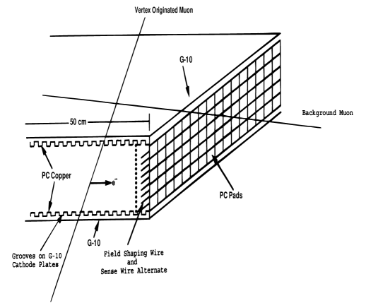
At high energy in the CoM, the channel becomes particularly attractive to study using the muon collider, if the forward going muons from the interaction can be detected [226]. The method provides a capability to search for any missing neutral state such as the Higgs boson via the missing mass technique. We are investigating methods to improve our forward muon detection capability.
X CONCLUSIONS
Unlike protons, muons are point-like but, unlike electrons, they emit relatively little synchrotron radiation and therefore can be accelerated and collided in rings.
Another advantage resulting from the low synchrotron radiation is the lack of beamstrahlung and the possibility of very small collision energy spreads. A beam energy spread of E/E of 0.003% is considered feasible for a 100 GeV machine. It has been shown that by observing spin precession, the absolute energy could be determined to a small fraction of this width. These features become important in conjunction with the large s-channel Higgs production (, 43000 times larger than for ), allowing precision measurements of the Higgs mass, width and branching ratios. A higher energy muon collider can also distinguish the nearly degenerate heavy Higgs bosons and of the minimal supersymmetric extension of the standard model, since these states can also be produced in the channel. We have also examined the ability of the muon collider to study techni-resonances, do a high luminosity study of boson physics, scan the and thresholds to make precision mass measurements as well as SUSY and strongly interacting W boson physics. The high luminosity proton driver and the cold low energy muons permit the study of rare kaon and muon decays. Muon storage rings will permit low-systematics studies of neutrino oscillations for a wide range of mixing angle and phase space with hitherto unattainable sensitivity.
Such machines are clearly desirable. The issues are:
-
whether they can be built and physics done with them
-
what they will cost.
Much progress has been made in addressing the first question and the answer, so far, appears to be yes. It is too early to address the second.
We have studied machines with CoM energies of 0.1, 0.4 and 3 TeV, defined parameters and simulated many of their components. Most recent work has been done on the 0.1 TeV First Muon Collider, the energy taken to be representative of the actual mass of a Higgs particle. A summary of progress and challenges follows:
a Proton driver
The specification of the proton driver for the three machines is assumed the same: protons/pulse at an energy above 16 GeV and 1-2 ns rms bunch lengths. There have been three studies of how to achieve these parameters. The most conservative, at 30 GeV, is a generic design. Upgrades of the FNAL (at 16 GeV) and BNL (at 24 GeV) accelerators have also been studied. Despite the very short bunch requirement, each study has concluded that the specification is attainable. Experiments are planned to confirm some aspects of these designs.
b Pion production and capture
Pion production has been taken from the best models available, but an experiment (BNL-E910) that has taken data, and is being analyzed, will refine these models. The assumed 20 T capture solenoid will require state-of-the-art technology. Capture, decay and phase rotation have been simulated, and have achieved the specified production of 0.3 muons per initial proton. The most serious remaining issues for this part of the machine are:
-
1.
The nature and material of the target: The baseline assumption is that a liquid metal jet will be used, but the effects of shock heating by the beam, and of the eddy currents induced in the liquid as it enters the solenoid, are not yet fully understood.
-
2.
The maximum rf field in the phase rotation: For the short pulses used, the current assumptions would be reasonably conservative under normal operating conditions, but the effects of the massive radiation from the nearby target are not known.
Both these questions can be answered in a target experiment planned to start within the next two years at the BNL AGS.
Polarization of the muon beams represents a significant physics advantage and is an important feature of a muon collider. Polarized muon beams are possible. Muons are produced with polarization in the rest frame of the pion, but they travel in all directions. By accepting the forward going muons, it is easy to obtain polarization in either beam easily. The amount of polarization can be increased with an accompanying price in luminosity.
c Cooling
The required ionization cooling is the most difficult and least understood element in any of the muon colliders studied. Ionization cooling is a phenomenon that occurs whenever there is energy loss in a strong focusing environment.
But achieving the nearly reduction required is a challenge. Cooling over a wide range has been simulated using lithium lenses and ideal (linear matrix) matching and acceleration. Examples of limited sections of solenoid lattices with realistic accelerating fields have now been simulated, but the specification and simulation of a complete system has not yet been done. Much theoretical work remains: space charge and wakefields must be included; lattices at the start and end of the cooling sequences must be designed; lattices including liquid lithium lenses must be studied, and the sections must be matched together and simulated as a full sequence. The tools for this work are nearly ready, and this project should be completed within two years.
Technically, one of the most challenging aspects of the cooling system appears to be:
-
High gradient rf (e.g. 36 MV/m at 805 MHz) operating in strong (5-10 T) magnetic field, with beryllium foils between the cavities.
An experiment is planned that will test such a cavity, in the required fields, in about two years time. On an approximately six year time scale, a Cooling Test Facility is being proposed that could test ten meter lengths of different cooling systems. If they are required, then an urgent need is to develop:
-
Lithium Lenses: (e.g. 2 cm diameter, 70 cm long, liquid lithium lenses with 10 T surface fields and a repetition rate of 15 Hz).
The use of 31 T solenoids could avoid their need, at least in the low energy First Muon Collider, which would ease the urgency of this rather long term R&D, but both options would require long-term R&D. Meanwhile a short lithium lens is under construction at BINP (Novosibirsk, Russia).
d Acceleration
The acceleration system is probably the least controversial, although possibly the most expensive, part of a muon collider. Preliminary parameters have been specified for acceleration sequences for a 100 GeV and a 3 TeV machine, but they need refinement. In the low energy case, a linac is followed by three recirculating or FFAG accelerators. In the high energy accelerator, the recirculating or FFAG accelerators are followed by three fast ramping synchrotrons employing alternating pulsed and superconducting magnets. The parameters do not appear to be extreme, and it does not appear as if serious problems are likely.
e Collider
The collider lattices are challenging because of the requirement of very low beta functions at the interaction point, high single bunch intensities, and short bunch lengths. However, the fact that all muons will decay after about 800 turns means that slowly developing instabilities are not a problem. Feasibility lattices have been generated for a 4 TeV case, and more detailed designs for 100 GeV machines are been studied. In the latter case, but still without errors, acceptances in both transverse and longitudinal phase space have been achieved in tracking studies. Beam scraping schemes have been designed for both the low energy (collimators) and high energy (septum extractors) cases.
The short bunch length and longitudinal stability problems are avoided if the rings, as specified, are sufficiently isochronous, but some rf is needed to remove the impedance generated momentum spread. Transverse instabilities (beam breakup) should be controlled by rf BNS damping.
The heating of collider ring superconducting magnets by electrons from muon decay can be controlled by thick tungsten shields, and this technique also shields the space surrounding the magnets from the induced radioactivity on the inside of the shield wall. A conceptual design of magnets for the low energy machine has been defined.
Although much work is yet to be done (inclusion of errors, higher order correction, magnet design, rf design, etc), the collider ring does not appear likely to present a serious problem.
f Neutrino radiation and detector background
Neutrino radiation, which rises as the cube of the energy, is not serious for machines with center of mass energies below about 1.5 TeV. It is thus not significant for the First Muon Collider; but above 2 TeV, it sets a constraint on the muon current and makes it harder to achieve desired luminosities. However, advances in cooling and correction of tune shifts may still allow a machine at 10 TeV with substantial luminosity ().
Background in the detector was at first expected to be a very serious problem, but after much work, shielding systems have evolved that limit most charged hadron, electron, gamma and neutron backgrounds to levels that are acceptable. Muon background, in the higher energy machines, is a special problem that can cause serious fluctuations in calorimeter measurements. It has been shown that fast timing and segmentation can help suppress this background, and preliminary studies of its effects on a physics experiment are encouraging. The studies are ongoing.
g Detector scenarios
We have considered several options for the experimental detector components for various CoM energy colliders. Much work needs to be done to optimize the physics reach at each energy by feeding back the results of detailed simulations of backgrounds and signal to the detector design. Only then will the feasibility of doing physics with a muon collider be fully explored.
h Summary
Much progress has been made since Snowmass, but much still needs to be done. A time scale of two years should allow completion of simulation studies and the experimental testing of crucial technical challenges. Prototype construction and testing will take another 4-6 years. The construction of a First Muon Collider by about 2010 does seems possible.
XI ACKNOWLEDGMENTS
This research was supported by the U.S. Department of Energy under Contracts No. DE-ACO2-98CH10886, DE-AC02-76CH03000 and DE-AC03-76SF00098.
REFERENCES
- [1] M. Tigner, Imperatives for Future High Energy Accelerators, AIP Conf. Proc. 279, p. 1 (1993).
- [2] G. I. Budker, Accelerators and Colliding Beams (in Russian), in Proc. 7th Int. Conf. on High Energy Accel. (Yerevan, 1969), p. 33; extract: AIP Conf. Proc. 352, p. 4 (1996).
- [3] G. I. Budker, Int. High Energy Conf. (Kiev, 1970), unpublished; extract: AIP Conf. Proc. 352, p. 4 (1996).
- [4] A. N. Skrinsky, Towards Ultimate Luminosity Polarized Muon Collider (Problems and Prospects), AIP Conf. Proc. 441, p. 249 (1998).
- [5] B. J. King, Discussion on Muon Collider Parameters at Center of Mass Energies from 0.1 TeV to 100 TeV, BNL-CAP-223-MUON-98C; to appear in Proc. EPAC98 Conf. (Stockholm, June 1998).
- [6] V. Bharadwaj, et al., Fermilab Collider Run 1b Accelerator Performance, Fermilab-TM-1970, (1995). See in particular Chapter 4, Table I (page 12) and Figure 8 (page 19); http://fnalpubs.fnal.gov/archive/1996/tm/TM-1970.html
- [7] M. D. Church and J. P. Marriner, The Antiproton Sources: Design and Operation Annu. Rev. Nucl. Sci., 43, p. 253 (1993)
- [8] A. A. Kolomensky, On the Oscillation Decrements in Accelerators in the Presence of Arbitrary Energy Losses, Sov. Atomic Energy 19, p. 1511 (1965); http://puhep1.princeton.edu/mumu/physics /kolomensky/1.html
- [9] G. I. Budker, An Effective Method of Damping Particle Oscillations in Proton and Antiproton Storage Rings, Sov. Atomic Energy 22, p. 438 (1967); http://puhep1.princeton.edu/mumu/physics/budker/1.html
- [10] Yu. M. Ado and V. I. Balbekov, Use of Ionization Friction in the Storage of Heavy Particles, Sov. Atomic Energy 31, p. 731 (1971); http://puhep1.princeton.edu/mumu/physics/ado/1.html
- [11] V. I. Balbekov, Achievable Transverse Emittance of Beam in Muon Collider, AIP Conf. Proc. 372, p. 140 (1996); ftp://ftp.mumu.bnl.gov/pub/documents/balbekov.ps
- [12] Rajendran Raja and Alvin Tollestrup, Calibrating the energy of a GeV Muon Collider using spin precession, Phys. Rev. D 58, 013005 (1998); http://xxx.lanl.gov/ps/hep-ex/9801004
- [13] D. Neuffer, Multi-TeV Muon Colliders, AIP Conf. Proc. 156, p. 201 (1987); http://www-ppd.fnal.gov/muscan/munotes/mc-006.pdf
- [14] S. Geer, Workshop on physics at the first muon collider and front end of a muon collider: A brief summary, in Ref. [40], p. 18.
- [15] A. N. Skrinsky, Intersecting Storage Rings at Novosibirsk, Proc. Int. Seminar on Prospects of High-Energy Physics (Morges, Mar. 1971), unpublished; extract: AIP Conf. Proc. 352, p. 6 (1996).
- [16] G. I. Budker and A. N. Skrinsky, Electron cooling and new possibilities in elementary particle physics, Sov. Phys. Usp. 21, p. 277 (1978).
- [17] A. N. Skrinsky, Acceleration and Instrumentation Prospects of Elementary Particle Physics, AIP Conf. Proc. 68, p. 1056 (1980).
- [18] A. N. Skrinsky and V. V. Parkhomchuk, Methods of cooling beams of charged particles, Sov. J. Part. Nucl. 12, p. 223 (1981).
- [19] A. N. Skrinsky, Accelerator and detector prospects of elementary particle physics, Sov. Phys. Usp. 25, p. 639 (1982), sec. 3n.
- [20] V. V. Parkhomchuk and A. N. Skrinsky, Ionization Cooling: Physics and Applications, in Proc. 12th Int. Conf. on High Energy Accel., ed. by F. T. Cole and R. Donaldson (Fermilab, 1983), p. 485; http://www-ppd.fnal.gov/muscan/munotes/mc-003.pdf
- [21] A. N. Skrinsky, Ionization Cooling and Muon Collider, AIP Conf. Proc. 372, p. 133 (1996).
- [22] A. N. Skrinsky, Polarized Muons Beams for Muon Collider, Nucl. Phys. B (Proc. Suppl.) 51A, p. 201 (1996).
- [23] D. Neuffer, Colliding Muons Beams at 90 GeV, Fermilab report FN-319 (July 1979); http://www-ppd.fnal.gov/muscan/munotes/mc-001.pdf
- [24] D. Neuffer, Principles and Applications of Muon Cooling, in Proc. 12th Int. Conf. on High Energy Accel., ed. by F. T. Cole and R. Donaldson (Fermilab, 1983), p. 481; Part. Acc. 14, p. 75 (1983); reproduced in AIP Conf. Proc. 353, 12 (1996).
- [25] D. Neuffer, colliders: possibilities and challenges in Ref. [27], p. 27.
- [26] J. Wurtele (ed.), Advanced Accelerator Concepts (Port Jefferson, NY, June 14-20, 1992), AIP Conf. Proc. 279 (1993); see P. Chen and K. T. McDonald, Summary of the Physics Opportunities Working Group, p. 853.
- [27] D. B. Cline (ed.), Proc. of the Mini-Workshop on Colliders (Napa, CA, Dec. 1992), Nucl. Instrum. & Methods A350, p. 24 (1994).
- [28] H. A. Thiessen (ed.), Proceedings of the Muon Collider Workshop, Los Alamos National Laboratory Report LA-UR-93-866 (Feb. 1993).
- [29] P. Schoessow (ed.), Advanced Accelerator Concepts (Fontana, WI, 1994), AIP Conf. Proc. 335 (1995); see R. B. Palmer, D. Neuffer and J. Gallardo, A Practical High-energy High-Luminosity Collider, p. 635.
- [30] D. B. Cline (ed.), Physics Potential and Development of Colliders (Sausalito, CA, Nov. 1994), AIP Conf. Proc. 352 (1996).
- [31] T. Tajima (ed.), The Future of Accelerator Physics, Proc. of the Tamura Symposium (Austin, TX, Nov. 1994), AIP Conf. Proc. 356 (1996); see D. V. Neuffer and R. B. Palmer, Progress Toward a High-Energy, High-Luminosity Collider, p. 344.
- [32] J. C. Gallardo (ed.), Beam Dynamics and Technology Issues for Colliders, 9th Advanced ICFA Beam Dynamics Workshop (Montauk, NY, Oct. 15-20, 1995), AIP Conf. Proc. 372 (1996).
- [33] D. G. Cassel, L. T. Gennari and R. H. Siemann (eds.), New Directions for High-Energy Physics, Proc. of the 1996 DPF/DPB Summer Study on High-Energy Physics, (Stanford Linear Accelerator Center, Menlo Park, CA, 1997).
- [34] Z. Parsa (ed.), Future High Energy Colliders (Santa Barbara, CA, Oct. 1996), AIP Conf. Proc. 397 (1997); see D. B. Cline, The Problems and Physics Prospects for a Collider, p. 203.
- [35] Workshop on Muon Colliders (LBNL, Feb. 1997).
- [36] Proc. 1997 Part. Accel. Conf. (PAC97) (Vancouver, Ca., 1997); http://www.triumf.ca/pac97/papers/
- [37] Mini-Workshop on the Muon Collider Lattice (BNL, 1997).
- [38] Mini-Workshop on Ionization Cooling (Fermilab, Oct. 1997).
- [39] S. Geer and R. Raja (eds.), Workshop on Physics at the First Muon Collider and at the Front End of the Muon Collider, (Fermilab, Nov. 1997), AIP Conf. Proc. 435 (1998); http://www.fnal.gov/projects/muon_collider/physics/talks.html
- [40] D. Cline (ed.), Proc. 4th Int. Conf. on the Physics Potential & Development of Colliders (San Francisco, CA, Dec. 10-12, 1997), AIP Conf. Proc. 441 (1998).
- [41] Muon Collider Collaboration meeting (Gulf Shores, AL, Mar. 1998).
- [42] Mini-Workshop on Ionization Cooling (BNL, 1998).
- [43] R. B. Palmer, A. Sessler and A. Tollestrup, Status Report of a High Luminosity Muon Collider and Future Research and Development Plans, in Ref. [33], p. 203; ftp://ftp.mumu.bnl.gov/pub/documents/aba_new.ps
- [44] The Collider Collaboration, Collider Feasibility Study, BNL-52503, FERMILAB-Conf-96/092, LBNL-38946 (July 1996); http://www.cap.bnl.gov/mumu/book.html
- [45] V. Barger, M. Berger, J. Gunion and T. Han, Higgs Boson Physics in the -Channel at Colliders, Phys. Rep. 286, 1 (1997); http://xxx.lanl.gov/hep-ph/9602397
- [46] J. Gunion, Physics at a Muon Collider, UCD-98-5 (Nov. 1997); http://xxx.lanl.gov/hep-ph/9802258
- [47] See the collection of articles at the URL http://www.fnal.gov/projects/muon_collider/physics/physics.html http://puhep1.princeton.edu/mumu/physics/
- [48] R. B. Palmer et al., Muon Collider Design, Nucl. Phys. B (Proc. Suppl.) 51A, p. 61 (1996).
- [49] R. B. Palmer et al., Muon Colliders, AIP Conf. Proc. 372, p. 3 (1996); http://xxx.lanl.gov/ps/acc-phys/960201
- [50] R. B. Palmer and J. C. Gallardo, Muon-Muon and Other High Energy Colliders, in Techniques and Concepts of High Energy Physics IX, ed. by T. Ferbel (Plenum Press, NY, 1997), p. 183; ftp://ftp.mumu.bnl.gov/pub/documents/master_stcroix.ps
- [51] R. B. Palmer and J. C. Gallardo, High Energy Colliders, in Critical Problems in Physics, ed. by V. L. Fitch, D. R. Marlow, M. A. E. Dementi (Princeton U. Press, Princeton, NJ, 1997), p. 247; http://xxx.lanl.gov/ps/physics/9702016
- [52] R. B. Palmer, Progress on Colliders, Proc. PAC97 (Vancouver, Ca., 1997), p. 286; http://www.triumf.ca/pac97/papers/pdf/6B002.PDF
- [53] R. B. Palmer, Muon Collider: Introduction and Status, BNL-65241, CAP-201-MUON-98C (Jan. 1998); http://xxx.lanl.gov/ps/physics/9802005
- [54] R. B. Palmer, Muon Collider Design, AIP Conf. Proc. 441, p. 183 (1998); http://xxx.lanl.gov/ps/physics/9802002.
- [55] R. Palmer, A. Sessler, A. Tollestrup and J. Gallardo, Muon Collider Overview: Progress and Future Plans, to appear in Proc. EPAC98 Conf. (Stockholm, June 1998); http://xxx.lanl.gov/ps/physics/9807006
- [56] A. G. Ruggiero, The Muon Collider, AIP Conf. Proc. 279, p. 958 (1993).
- [57] S. Geer, The Physics Potential of Neutrino Beams from Muon Storage Rings, AIP Conf. Proc. 435, p. 384 (1998); http://www.fnal.gov/projects/muon_collider/talks/steves_nu_talk.ps
- [58] S. Geer, Muon Storage Ring Neutrino Source, presented at Int. Workshop on JHF Science (KEK, March, 1998); http://www.fnal.gov/projects/muon_collider/talks/sg_nu_jhf98.ps
- [59] S. Geer, Neutrino beams from muon storage rings: Characteristics and physics potential, Phys. Rev. D57, p. 6989 (1998).
- [60] R. Mohapatra, Neutrino Physics in a Muon Collider, AIP Conf. Proc. 435, 358 (1998); http://xxx.lanl.gov/ps/hep-ph/9711444.
- [61] D. A. Harris, and K. S. McFarland, Detectors for Neutrino Physics at the First Muon Collider, AIP Conf. Proc. 435, p. 376 (1998); http://xxx.lanl.gov/ps/hep-ex/9804010.
- [62] B. J. King, Neutrino Physics at a Muon Collider, AIP Conf. Proc. 435, p. 334 (1998); http://pubweb.bnl.gov/people/bking/nufnal97.ps
- [63] B. J. King, Neutrino Physics at Muon Colliders, AIP Conf. Proc. 441, p. 132 (1998); http://pubweb.bnl.gov/people/bking/sf97.ps
- [64] B. J. King, Muon Colliders: New Prospects for Precision Physics and the High Energy Frontier, BNL report CAP-224-MUON-98C (April, 1998), submitted to Proc. Latin Am. Symp. High Energy Phys. (San Juan, Puerto Rico, April 8-11, 1998); http://pubweb.bnl.gov/people/bking/pr98.ps
- [65] J. Yu and A. V. Kotwal, Measurements of at the First Muon Collider, AIP Conf. Proc. 435, 398 (1998).
- [66] D. Cline and D. Neuffer, A Muon Storage Ring for Neutrino Oscillation Experiments, AIP Conf. Proc. 68, p. 846 (1980); reproduced in AIP Conf. Proc. 352, p. 10 (1996);
- [67] V. Barger, M. S. Berger, J. F. Gunion and T. Han, s-Channel Higgs Boson Production at a Muon-Muon Collider, Phys. Rev. Lett. 75, p. 1462 (1995).
- [68] E. Richter-Was, D. Froidevaux, F. Gianotti, L. Poggioli, D. Cavalli, S. Resconi, CERN-TH-96-111 (1996).
- [69] C. T. Hill, Topcolor assisted technicolor, Phys. Lett. B345, 483 (1995); K. Lane and E. Eichten, Natural topcolor-assisted technicolor, Phys. Lett. B352, 382 (1995); K. Lane, Symmetry breaking and generational mixing in top-color-assisted technicolor, Phys. Rev. D54, 2204 (1996).
- [70] R. Casalbuoni et al., The pseudo-Goldstone mass spectrum, Phys. Lett. B285, 103 (1992).
- [71] P. Bhat and E. Eichten, FERMILAB-CONF-98/072; K. Lane, BUHEP-98-01, http://xxx.lanl.gov/ps/hep-ph/9810385, in Ref. [39]; J. Womersley, Technihadron Production at a Muon Collider, AIP Conf. Proc. 435, 754 (1998); D. Dobrescu and C. T. Hill, FERMILAB-PUB-97/409-T, http://xxx.lanl.gov/ps/hep-ph/9712319; R. Casalbuoni et al., http://xxx.lanl.gov/ps/hep-ph/9801243, in Ref. [39]; J. F. Gunion, UCD-98-5, http://xxx.lanl.gov/ps/hep-ph/9802258; R. Casalbuoni et al., UCD-98-13.
- [72] J. F. Gunion, Probing exotic Higgs sectors in collisions, Int. J. of Mod. Phys. A13, 2277 (1997), and references therein.
- [73] J. L. Feng, J. F. Gunion, and T. Han, R-Parity violation and sneutrino resonances at muon colliders, http://xxx.lanl.gov/ps/hep-ph/9711414.
- [74] M. DeMarteau and T. Han, FERMILAB-CONF-98/030, http://xxx.lanl.gov/ps/hep-ph/9801407, in Ref. [39].
- [75] J. Erler and P. Langacker, Electroweak Model and Contraints on New Physics, Eur. Phys. J., C3, 1 (1998), p. 90; http://pdg/lbl.gov.
- [76] V. Barger, M. S. Berger, J. F. Gunion and T. Han, Precision W-boson and top-quark mass determinations at a muon collider, Phys. Rev. D56, 1714 (1997); Precision Higgs Boson Mass Determination at Lepton Colliders,Phys. Rev. Lett. 78, 3991 (1997).
- [77] S. Parke, Top Quark Physics at a Polarized Muon Collider, http://xxx.lanl.gov/ps/hep-ph/9802279.
- [78] See e.g., M. Carena and S. Protopopescu, in Ref. [39].
- [79] H. Baer, C. Chen, C. Kao, and X. Tata, Supersymmetry reach of an upgraded Fermilab Tevatron Collider, Phys. Rev. D52, 1565 (1995).
- [80] V. Barger, M.S. Berger, and T. Han, Chargino mass determination at a muon collider, University of Wisconsin-Madison report MADPH-98-1036 http://xxx.lanl.gov/ps/hep-ph/9801410.
- [81] I. Hinchliffe, in Ref. [39].
- [82] F. Paige, in Ref. [39].
- [83] V. Barger, M. S. Berger, J. F. Gunion, and T. Han, in Proceedings of the Symposium on Physics Potential and Development of Colliders, San Francisco, CA (1995), D. Cline and D. Sanders (eds.), Nucl. Phys. B (proc. suppl.) 51A, 13 (1996).
- [84] J. Lykken, Sparticle Masses from Kinematic Fitting at a Muon Collider, http://xxx.lanl.gov/ps/hep-ph/9803427.
- [85] S. Godfrey, New Particles and Interactions at High Energy Muon Colliders, http://xxx.lanl.gov/ps/hep-ph/9802212.
- [86] V. Barger, M. S. Berger, J. F. Gunion and T. Han, Studying a strongly interacting electroweak sector via longitudinal gauge-boson scattering at a muon collider, Phys. Rev. D55, 142 (1997).
- [87] W. J. Marciano, Low Energy Physics and the First Muon Collider in Ref. [39], p. 58; W. Molzon, Physics with Low Energy Muons at the Front End of the Muon Collider ibid, p. 152.
- [88] C. Ankenbrandt and S. Geer, Accelerator scenario and parameters for the first muon collider and front end of a muon collider, in Ref. [39], p. 3.
- [89] Kingman Cheung, Muon-proton Colliders: Leptoquarks and Contact Interactions http://xxx.lanl.gov/ps/hep-ph/9802219, in Ref. [39].
- [90] J. Norem et al., The Proton Driver for the Collider, Proc. PAC97 (Vancouver, Ca., 1997), p. 399; http://www.triumf.ca/pac97/papers/pdf/4W025.PDF
- [91] TRIUMF, KAON Factory Proposal, Triumf, Sept. 1985.
- [92] 5 MW Pulsed Spallation Neutron Source, Preconceptual Design Study, BNL-60678 (June 1994).
- [93] Chapter 3 of Ref. [44].
- [94] C. Ankenbrandt and R. Noble, Summary of the Accelerator Working Group, AIP Conf. Proc. 435, 3 (1998); http://www-lib.fnal.gov/archive/1998/conf/Conf-98-074.html
- [95] M. Blaskiewicz et al., High Intensity Proton Operations at Brookhaven, in Proc. 1995 Part. Accel. Conf. (PAC95) (Dallas, TX, 1995), p. 383.
- [96] T. Roser, AGS Performance and Upgrades: A Possible Proton Driver for a Muon Collider, AIP Conf. Proc. 372, 47 (1996); ftp://ftp.mumu.bnl.gov/pub/documents/roser.ps
- [97] L. Ahrens et al., High Intensity Proton Acceleration at the Brookhaven AGS – An Update, Proc. PAC97 (Vancouver, Ca., 1997), p. 89; http://www.triumf.ca/pac97/papers/pdf/7P001.PDF
- [98] T. Roser, High Intensity Performance and Upgrades at the Brookhaven AGS, Proc. Workshop on Space Charge Physics in High Intensity Hadron Rings, (Shelter Island, NY, May 4–7, 1998), to be published.
- [99] Y. Cho et al., A 10-GeV, 5-MW Proton Source for a Muon-Muon Collider, AIP Conf. Proc. 372, 31 (1996); ftp://ftp.mumu.bnl.gov/pub/documents/harkay.ps
- [100] S. D. Holmes (ed.), A Development Plan for the Fermilab Proton Source, FERMILAB-TM-2021 (Sept. 1997); http://www-lib.fnal.gov/archive/1997/tm/c-TM-2021.pdf
- [101] M. Popovic (ed.), Present, Near Future and Future Performance of the Fermilab Linac, FERMILAB-Pub-96/046 (March 1996); http://www-lib.fnal.gov/archive/1996/pub/Pub-96-046.html
- [102] K. Y. Ng and Z. Qian, Space-Charge Effects of the Proposed High-Intensity Fermilab Booster, FERMILAB-Conf-98-116 (April 1998); http://www-lib.fnal.gov/archive/1998/conf/Conf-98-116.html
- [103] J. E. Griffin, RF System Considerations for the Muon Collider Proton Driver Synchrotrons, FERMILAB-FN-669 (June 1998); http://www-lib.fnal.gov/archive/1998/fn/FN-669.html
- [104] C. Ankenbrandt et al., Bunching Near Transition in the AGS, Phys. Rev. ST Accel. Beams 1, 030101 (1998); http://www-lib.fnal.gov/archive/1998/pub/Pub-98-006.html
- [105] J. Norem et al., An AGS experiment to test bunching for the proton driver of the muon collider, ANL-HEP-CP-98-32 (May 1998); J. Norem et al., Bunch Shortening Experiments in the Fermilab Booster and the AGS, Proc. PAC97 (Vancouver, Ca., 1997), p. 396; http://www.triumf.ca/pac97/papers/pdf/4W024.PDF
- [106] D. Trbojevic et al., A Proton Driver for the Muon Collider Source with a Tunable Momentum Compaction Lattice, Proc. PAC97 (Vancouver, Ca., 1997), p. 1030; http://www.triumf.ca/pac97/papers/pdf/7W017.PDF
- [107] J. E. Griffin, K. Y. Ng, Z. B. Qian and D. Wildman, Experimental Study of Passive Compensation of Space Charge Potential Well Distortion at the Los Alamos National Laboratory Proton Storage Ring, FERMILAB-FN-661 (Dec. 1997); http://www-lib.fnal.gov/archive/1997/fn/FN-661.html
- [108] J. E. Griffin et al., IEEE Trans. Nucl. Sci. NS–30, 3502 (1983).
- [109] J. M. Brennan and M. M. Blaskiewicz, Proc. Workshop on Space Charge Physics in High Intensity Hadron Rings, (Shelter Island, NY, May 4–7, 1998), to be published.
- [110] N. Mokhov, R. Noble and A. Van Ginneken, Target and Collection Optimatization for Muon Colliders, AIP Conf. Proc. 372, 61 (1996); http://www-lib.fnal.gov/archive/1996/conf/Conf-96-006.html
- [111] N. V. Mokhov and A. Van Ginneken, Pion Production and Targetry at Colliders, FERMILAB-Conf-98/041 (Jan. 1998); http://www-lib.fnal.gov/1998/archive/conf/Conf-998-041.html.
- [112] D. Ehst, N. V. Mokhov, R. J. Noble and A. Van Ginneken, Target Options and Yields for a Muon Collider Source, Proc. PAC97 (Vancouver, Ca., 1997), p. 393; http://www.triumf.ca/pac97/papers/pdf/4W023.PDF
- [113] H. Takahashi, Y. An, X. Chen and M. Nomura, Optimization of the Target for Muon Colliders, Proc. PAC97 (Vancouver, Ca., 1997), p. 402; http://www.triumf.ca/pac97/papers/pdf/4W027.PDF
- [114] S. H. Kahana, Y. Pang and T. J. Schlagel, in Proc. Heavy Ion Physics at the AGS - HIPAGS ’93, ed. by G. S. F. Stephans et al.; D. Kahana and Y. Torun, Analysis of Pion Production Data from E-802 at 14.6 GeV/ Using ARC, BNL-61983 (July 1995); http://bnlnth.phy.bnl.gov/arc/arc.html http://www-pat.fnal.gov/muSim/ARC.html
- [115] N. V. Mokhov, The MARS Code System User’s Guide, Version 13(98), FERMILAB-FN-628 (Feb. 1998); http://www-ap.fnal.gov/MARS/
- [116] N. V. Mokhov and S. I. Striganov, Model for Pion Production in Proton-Nucleus Interactions, FERMILAB-Conf-98-053 (Feb. 1998); http://www-lib.fnal.gov/archive/1998/conf/Conf-98-053.html
- [117] J. Ranft, DPMJET version II.3 and II.4, INFN-AE-97-45 (1997); http://preprints.cern.ch/cgi-bin/setlink?base=preprint&categ=scan&id=SCAN-9711078.
- [118] Experiment E-910 at BNL-AGS; http://www.nevis.columbia.edu/heavyion/e910/
- [119] Hiroyoshi Hiejima, Columbia University (heijima@nevis1.columbia.edu), private communication.
- [120] R. B. Palmer et al.,, Monte Carlo Simulations of Muon Production, AIP Conf. Proc. 352, 108 (1996); ftp://ftp.mumu.bnl.gov/pub/documents/monte1.ps
- [121] J. Lettry et al., Experience with ISOLDE Molten Metal Targets at the CERN-PS Booster, in Proceedings of ICANS-XIII (1995); http://puhep1.princeton.edu/mumu/target/lettry/1.html
- [122] C. Johnson, Solid and Liquid Targets Overview, http://nicewww.cern.ch/ cdj/public/mumutarg/
- [123] L. Ni and G. Bauer, Dynamic Stress of a Liquid Metal Target Container under Pulsed Heating, PSI prpeprint (1998); http://puhep1.princeton.edu/mumu/target/bauer/1.html
- [124] C. Lu and K. T. McDonald, Low-Melting-Temperature Metals for possible Use as Primary Targets at a Muon Collider Source, Princeton//97-3 (May 1998); http://www.hep.princeton.edu/mumu/mumu-97-3.ps
- [125] R. Weggel, Deceleration of Conductor by Magnetic Field: 1) Paraxial; 2) Perpendicular, BNL report CAP-220-MUON-98R (1998).
- [126] C. Lu and K. T. McDonald, Flowing Tungsten Powder for Possible Use as the Primary Target at a Muon Collider Source, Princeton//98-10 (Mar. 15, 1998); http://www.hep.princeton.edu/mumu/mumu-98-10.ps
- [127] B. J. King, N. V. Mokhov and R. Weggel, A Cu-Ni Rotating Band Target for Pion Production at Muon Colliders (April 1998); http://pubweb.bnl.gov/people/bking/talks.html
- [128] R. Weggel, 4-MW Hollow-Conductor Magnets for 20 T Hybrid Systems to Collect Pions for a Muon Collider, BNL report MU-015 (Jan. 1997).
- [129] J. R. Miller et al., An Overview of the 45-T Hybrid Magnet System for the New National High Magnetic Field Laboratory, IEEE Transactions on Magnetics 30, 1563 (1994).
- [130] R. B. Palmer and J. C. Gallardo, MC: Fortran program to simulate the front end and cooling section, unpublished.
- [131] see p. 220 of Ref. [44].
- [132] K. Assamagan et al., Measurement of the muon momentum in pion decay at rest using a surface muon beam, Phys. Lett. B335, 231 (1994).
- [133] E. P. Wigner, On Unitary Representation of the Inhomogeneous Lorentz Group, Ann. Math. 40, 149 (1939).
- [134] E. P. Wigner, Relativistic Invariance and Quantum Phenomena, Rev. Mod. Phys. 29, 255 (1957).
- [135] B. Norum and R. Rossmanith, Polarized beams in a muon collider, Nucl. Phys. B (Proc. Suppl.) 51A, 191 (1996).
- [136] J. Alessi et al., An R&D Program for Targetry at a Muon Collider, proposal to the BNL AGS (Sept. 1998); http://puhep1.princeton.edu/mumu/target/targetprop.ps
- [137] A. A. Mikhailichenko and M. S. Zolotorev, Optical Stochastic Cooling, Phys. Rev. Lett. 71, 4146 (1993).
- [138] A. Hershcovitch, Some Options for Pion and Muon Focusing in the AGS g-2 and Neutrino Oscillation Experiments (and Possible New Focusing and Cooling Schemes for a Muon Collider), AGS/AD Tech. Note No. 413 (BNL, Feb. 1996); High Current Magnetized Plasma Discharges and Electron Beams for Capture and Cooling of Charged Leptons and Hadrons, Proc. PAC97 (Vancouver, Ca., 1997), p. 1792; http://www.triumf.ca/pac97/papers/pdf/4V024.PDF
- [139] P. Chen, Z. Huang and R. Ruth, Radiation and Radiation Reaction in Continuous Focusing Channels, AIP Conf. Proc. 335, 646 (1995).
- [140] P. H. Sandler, S. A. Bogacz and D. B. Cline, Muon Cooling and Acceleration Experiment using Muon Sources at TRIUMF, AIP Conf. Proc. 352, 146 (1996).
- [141] Chapter 6 of Ref. [44].
- [142] R. C. Fernow and J. C. Gallardo, Muon transverse ionization cooling: Stochastic approach, Phys. Rev. E 52, 1039 (1995); ftp://ftp.mumu.bnl.gov/pub/documents/stochastic.ps
- [143] R. C. Fernow and J. C. Gallardo, Validity of the differential equations for ionization cooling, AIP Conf. Proc. 352, 170 (1996).
- [144] Particle Data Group, Review of Particle Physics, Eur. Phys. J. C 3, 1 (1998), p. 138; http://pdg/lbl.gov
- [145] A. Van Ginneken, Fluctuations of muon energy loss and simulation of ionization cooling, Nucl. Instrum. & Methods A362, 213 (1995).
- [146] R. Fernow, ICOOL: Fortran program to simulate muon ionization cooling, unpublished; http://pubweb.bnl.gov/people/fernow/readme.html http:/www-pat.fnal.gov/muSim/icool.html
- [147] H. Kirk, Parmela modeling of alternating solenoids, presented at [42] (1998).
- [148] GEANT manual, v.3.2.1, CERN program Library W5013 (CERN, 1994); http://wwwinfo.cern.ch/asdoc/geant_html3/geantall.html
- [149] P. Lebrun, Alternate solenoid in DPGeant, presented at [42] (1998).
- [150] C. M. Celata, A. M. Sessler, P. B. Lee, B. A. Shadwick and J. S. Wurtele, A moment expansion approach to a muon collider cooling lattice, to appear in Proc. EPAC98 Conf. (Stockholm, June 1998).
- [151] R. B. Palmer, The Angular Momentum Problem, or Why We Reverse the Solenoids, BNL-CAP-MU-022 (1998); http://pubweb.bnl.gov/people/palmer/notes/whyalt.ps.
- [152] G. Silvestrov, in Ref. [28].
- [153] B. Bayanov et al., A Lithium Lens for Axially Symmetric Focusing of High Energy Particle Beams, Nucl. Instrum. & Methods 190, 9 (1981).
- [154] C. D. Johnson, Present and Future Possibilities of Antiproton Production from Fixed Targets at CERN, Hyperfine Interactions 44, 21 (1988).
- [155] G. Silvestrov, Lithium Lenses for Muon Colliders, AIP Conf. Proc. 372, 168 (1996); ftp://ftp.mumu.bnl.gov/pub/documents/greg.ps
- [156] V. Balbekov and A. Van Ginneken, presented at [38] (Oct. 1997).
- [157] V. Balbekov and A. Van Ginneken, Ring Cooler for Muon Collider, AIP Conf. Proc. 441, p. 310 (1998).
- [158] R. C. Fernow, J. C. Gallardo, H. G. Kirk and R. B. Palmer, Transverse Cooling in the Muon Collider, submitted to Proc. 8th Workshop on Advanced Accelerator Concepts (Baltimore, MD, July 5-11, 1998); http://pubweb.bnl.gov/people/fernow/reports/asol.ps
- [159] J. C. Gallardo, R. C. Fernow and R. B. Palmer, Muon Dynamics in a Toroidal Sector Magnet, AIP Conf. Proc. 441, p. 282 (1998).
- [160] D. Neuffer, Phase Space Exchange in Thick Wedge Absorbers for Ionization Cooling, AIP Conf. Proc. 441, p. 270 (1998).
- [161] D. Neuffer and A. Van Ginneken, presented at [42] (Jan. 1998).
- [162] D. Neuffer and W. Wan, COSY transport for cooling, presented at [38] (Oct. 1997).
- [163] C. N. Ankenbrandt et al., Ionization Cooling Research and Development Program for a High Luminosity Muon Collider, Fnal-P904 (April 15, 1998); http://www.fnal.gov/projects/muon_collider/
- [164] S. Geer, Ionization Cooling Research and Development Program for a High Luminosity Muon Collider, FERMILAB-Conf-98/136, presented at the International Workshop on JHF Science (JHF98), KEK, Tsukuba-shi, Ibaraki, Japan; http://fnalpubs.fnal.gov/archive/1998/conf/Conf-98-136.html
- [165] C. Lu, K. T. McDonald, E. J. Prebys and S. E. Vahsen, A Detector Scenario for the Muon Cooling Experiment, Princeton//97-8 (May, 1998); http://www.hep.princeton.edu/mumu/mumu-97-8.ps
- [166] F. Mills, FNAL (fredmills@aol.com), private communication.
- [167] B. J. King, Variable Field Bending Magnets for Recirculating Linacs, BNL-CAP-MU-023, 1998; http://pubweb.bnl.gov/people/bking/magnet.ps
- [168] D. Neuffer, Analyses and simulations of longitudinal motion in -recirculating linacs, Nucl. Instrum. and Methods A384, 263 (1997).
- [169] D. V. Neuffer, Acceleration to Collisions for the Collider, AIP Conf. Proc. 372, 315 (1996); ftp://ftp.mumu.bnl.gov/pub/documents/aclmntk.ps
- [170] D. Summers, D. Neuffer, Q.-S. Shu and E. Willen, Acceleration for the Collider, Proc. PAC97 (Vancouver, Ca., 1997), p. 624; http://www.triumf.ca/pac97/papers/pdf/3PC004.PDF
- [171] D. J. Summers, Hybrid Rings of fixed 8 T Superconducting Magnets and Iron Magnets Rapidly Cycling between T and T for a Muon Collider, in Ref. [33], p. 238.
- [172] TESLA Collaboration, TESLA Test Facility Linac-Design Report, ed. by D. Edwards, TESLA 95-01 (1995).
- [173] Z. D. Farkas et al., SLED: A Method of Doubling SLAC’s Energy, SLAC-PUB-1435; in Proc. of the 9th Int. Conf. on High Energy Accelerators (Stanford, CA, 1974), p. 576.
- [174] E. Willen, Pulsed Dipole Magnets for the Muon Collider, Magnet Note 555-31 (BNL, May 1996); also in Ref. [33], p. 246.
- [175] Allied Signal, Amorphous Metals Division, 6 Eastmans Road, Parsippany, NJ 07054.
- [176] Magnetics, Division of Spang & Company, 900 East Butler Road, Butler, PA 16003.
- [177] I. Campisi, Jefferson Lab, (campisi@jlab.org), private communication.
- [178] A. Mosnier and O. Napoly, Wakefield effects in a Superconducting Linear Collider, Int. J. Mod. Phys. A (Proc. Suppl.) 2B, 963 (1993).
- [179] A. Novokhatski and A. Mosnier, Wakefield Dynamics in Quasiperiodic Structures, Proc. PAC97 (Vancouver, Ca., 1997), p. 467; http://www.triumf.ca/pac97/papers/pdf/8W013.PDF
- [180] V. Balakin, A. Novokhatsky and V. Smirnov, VLEPP: Transverse Beam Dynamics in Proc. 12th Int. Conf. on High Energy Accel., ed. by F. T. Cole and R. Donaldson (Fermilab, 1983), pag. 119;
- [181] A. Chao, Physics of Collective Beam Instabilities in High Energy Accelerators (John Wiley & Sons, Inc., New York, 1993).
- [182] K. L. Brown and J. Spencer, Nonlinear Optics for the Final Focus of the Single Pass Collider, IEEE Trans. Nucl. Sci. NS28, 2568 (1981).
- [183] K. L. Brown, Basic Optics of the SLC Final Focus System, SLAC-PUB-4811 (Dec. 1988).
- [184] K. L. Brown J. J. Murray and T. H. Fieguth, The Completed Design of the SLC Final Focus System, SLAC-PUB-4219 (Feb. 1987); http;//ccdb1.kek.jp/cgi-bin/img_index?8706254
- [185] O. Napoly, CLIC Final Focus System: Upgraded Version with Increased Bandwidth and Error Analysis, CLIC Note 227 (CERN, 1994).
- [186] C. Johnstone et al., An Isochronous Lattice Design for a 50 on 50 GeV Muon Collider, AIP Conf. Proc. 441, p. 209 (1998).
- [187] C. J. Johnstone and N. V. Mokhov, Optimization of a Muon Collider Interaction Region with Respect to Detector Backgrounds and the Heat Load to the Cryogenic Systems, in Ref. [33], p. 226; FERMILAB-Conf-96-366 (1996); http://www-lib.fnal.gov/archive/1996/conf/Conf-96-366.html
- [188] A. Drozhdin et al., Scraping Beam Halo in Colliders, AIP Conf. Proc. 441, p 242 (1998); FERMILAB-Conf-98/042 (1998); http://www-lib.fnal.gov/archive/1998/conf/Conf-98-042.html
- [189] M. Donald et al., Localized Chromaticity Correction of Low-Beta Insertions in Storage Rings, Proc. 1993 Part. Accel. Conf. (Washington, D.C., 1993), p. 131.
- [190] W. Wan and C. Johnstone, Tracking simulations of local, interleaved and noninterleaved chromatic correction sextupoles, presented at [37] (1997).
- [191] K.-Y. Ng, S.Y. Lee and D. Trbojevic, FNAL-FN595 (Fermilab, 1992).
- [192] S. Y. Lee, K. Y. Ng and D. Trbojevic, Minimizing dispersion in flexible-momentum-compaction lattices, Phys. Rev. E 48, 3040 (1993).
- [193] M. Berz, COSY INFINITY, V. 8. User’s Guide and Reference Manual (Nov. 1997); http://www.beamtheory.nscl.msu.edu/cosy/
- [194] S. Ohnuma, ohnuma@uh.edu, Inst. for Beam Particle Dynamics; Rm. 632 SR1; Houston, TX 99204-5506, private communication.
- [195] N. Merminga and K.Y. Ng, Hamiltonian Approach to Distortion Functions, Fermilab Report FN-493, 1988.
- [196] Y. T. Yan, SLAC (yan@slac.stanford.edu), private communication.
- [197] L. Schachinger and R. Talman, TEAPOT: A Thin-Element Accelerator Program for Optics and Tracking, Part. Accel. 22, 35 (1987).
- [198] G. W. Foster and N. V. Mokhov, Backgrounds and Detector Performance at a TeV Collider, AIP Conf. Proc. 352, 178 (1996).
- [199] M. Furman, The Classical Beam-Beam Interaction for the Muon Collider: A First Look, BF-19/CBP-Note-169/LBL-38563 (1996).
- [200] P. Chen, Beam-beam interaction in muon colliders, Nucl. Phys. B (Proc. Suppl.) 51A, 179 (1996).
- [201] W.-H. Cheng, A. M. Sessler and J. Wurtele, Studies of Collective Instabilities in Muon Collider Rings, AIP Conf. Proc. 372, 206 (1996).
- [202] K. Y. Ng, Beam stability Issues in a Quasi-Isochronous Muon Collider, AIP Conf. Proc. 372, 224 (1996).
- [203] N. V. Mokhov and S. I. Striganov, Simulation of Backgrounds in Detector and Energy Deposition in Superconducting Magnets at Colliders, AIP Conf. Proc. 372, 234 (1996); http://www-lib.fnal.gov/archive/1996/conf/Conf-96-011.html
- [204] E. Willen et al., A Helical Magnet Design for RHIC, Proc. PAC97 (Vancouver, Ca., 1997), p. 3362; http://www.triumf.ca/pac97/papers/pdf/3P010.PDF
- [205] T. Roser (Spokesperson) et al., Conceptual Design for the Acceleration of Polarized Protons in RHIC (Feb. 1995); http://www.ags.bnl.gov/roser/cdr07034/cdr07034.html
- [206] E. Willen, BNL (willen@bnl.gov), private communication.
- [207] N. V. Mokhov, Radiation Issues of a Collider, FERMILAB-Conf-96/367 (Oct. 1996); http://www-lib.fnal.gov/archive/1996/conf/Conf-96-367.html
- [208] The Physics Opportunities and Technical Challenges of a Muon Collider, BNL-CAP-MU-024; http://pubweb.bnl.gov/people/bking/1996/.
- [209] B. J. King, Neutrino Radiation Hazard at Muon Colliders, presented at [35] (Feb. 1997).
- [210] B. J. King, A Characterization of the Neutrino-Induced Radiation Hazard at TeV-Scale Muon Colliders, BNL report CAP-162-MUON-97R (1997).
- [211] B. J. King, Neutrino Radiation at Muon Colliders (April 1998); http://pubweb.bnl.gov/people/bking/nurad_aps98/
- [212] Particle Data Group, Review of Particle Physics, Eur. Phys. J. C 3, 1 (1998), p. 163; http://pdg/lbl.gov
- [213] C. Johnstone and N. Mokhov, Shielding the Muon Collider Interaction Region, Proc. PAC97 (Vancouver, Ca., 1997),p. 414; http://www.triumf.ca/pac97/papers/pdf/4W030.PDF
- [214] K. V. Lotov, A. N. Skrinsky and A. V. Yashin, Plasma Supression of Beam-Beam Interaction in a Muon Collider, Budker INP 98-41.
- [215] I. Stumer et al., Study of Detector Backgrounds at a Muon Collider, in Ref. [33], p. 463.
- [216] N. V. Mokhov, Comparison of backgrounds om detectors for LHC, NLC and colliders, Nucl. Phys. B (Proc. Suppl.) 51A, 210 (1996); http://fnalpubs.fnal.gov/archive/1996/conf/Conf-96-062.html
- [217] Sec. 8.5.3 of Ref. [44],
- [218] I. Ginzburg, The pair production at collider, Nucl. Phys. B (Proc. Suppl.) 51A, 186 (1996); http://xxx.lanl.gov/ps/hep-ph/9601273
- [219] S. Geer, Backgrounds and detector issues at a muon collider, in Ref. [33].
- [220] The SLD collaboration, The SLD CCD vertex detector and its upgrade, Nuovo Cimento 109A, 1027 (1996).
- [221] E. Gatti and P. Rehak, Semiconductor Drift Chamber - An Application of a Novel Charge Transport Scheme, Nucl. Instrum. & Methods, 225, 608 (1984).
- [222] Sherwood I. Parker, Christopher J. Kenney, Julie Segal, 3D: A New Architecture for Solid State Radiation Detectors, UH-511-839-96, 24pp. Submitted to Nucl. Instrum. & Methods.
- [223] S. Geer and J. Chapman, The Pixel Micro-Telescope, in Ref. [33], FERMILAB-CONF-96-375.
- [224] Sec. 9.4.2 of Ref. [44].
- [225] M. Atac, Directional muon jet chamber for a muon collider (groovy chamber), FERMILAB-CONF-96-401, Oct. 1996. Presented at the 1996 DPF/DPB Summer Study on New Directions for High-Energy Physics (Snowmass96).
- [226] R. Raja, A Feasibility Study of the Channel Using the Missing Mass Technique at the 4 TeV in the Center of Mass, Fermilab Muon Collider Note MC-042, April 1997.