Numerical approximations using Chebyshev polynomial expansions: El-gendi’s method revisited

Abstract

We present numerical solutions for differential equations by expanding the unknown function in terms of Chebyshev polynomials and solving a system of linear equations directly for the values of the function at the extrema (or zeros) of the Chebyshev polynomial of order $N$ (El-gendi’s method). The solutions are exact at these points, apart from round-off computer errors and the convergence of other numerical methods used in solving the linear system of equations. Applications to initial value problems in time-dependent quantum field theory, and second-order boundary value problems in fluid dynamics are presented.

I Introduction

A major problem in modern physics is to understand the time evolution of a quark-gluon plasma produced following a relativistic heavy-ion collision. Although a mean field theoretical approach ref:Hartree ; ref:GV ; ref:LOLN can provide a reasonable picture of the phase diagram of quantum field theories, such studies do not include a rescattering mechanism, which would allow an out of equilibrium system to be driven back to equilibrium. As such, the past few years have witnessed a major effort concerning the search for approximation schemes ref:EQT ; ref:abw ; ref:ctpN ; ref:berges which go beyond mean field theory. In the process, new numerical techniques were required in order to solve the ever more challenging systems of complex integro-differential equations.

In this paper we revive and extend an old spectral method based on expanding the unknown function in terms of Chebyshev polynomials, which plays a crucial role in implementing our non-equilibrium field theory program. Finite-difference methods, though leading to sparse matrices, are notoriously slowly convergent. Thus the need to use higher-order methods, like the nonuniform-grid Chebyshev polynomial methods, which belong to a class of spectral numerical methods. Then the resulting matrices are less sparse, but what is apparently lost in storage requirements, is regained in speed. We do in fact keep the storage needs moderate, as we can achieve very good accuracy with a moderate number of grid points.

The Chebyshev polynomials of the first kind of degree $n$, $T_{n}(x)$ with $n\leq N$, satisfy discrete orthogonality relationships on the grid of the extrema of $T_{N}(x)$. Based on this property, Clenshaw and Curtis ref:Clenshaw proposed almost forty years ago a quadrature scheme for finding the integral of a non-singular function defined on a finite range, by expanding the integrand in a series of Chebyshev polynomials and integrating this series term by term. Bounds for the errors of the quadrature scheme have been discussed in ref:errors1 and reveal that by truncating the series at some order $m<N$ the difference between the exact expansion and the truncated series can not be bigger than the sum of the neglected expansion coefficients ref:nr . This is a consequence of the fact that the Chebyshev polynomials are bounded between $\pm 1$, and if the expansion coefficients are rapidly decreasing, then the error is dominated by the $m+1$ term of the series, and spreads out smoothly over the interval $[-1,1]$.

Based on the discrete orthogonality relationships of the Chebyshev polynomials, various methods for solving linear and nonlinear ordinary differential equations ref:ode1 and integral differential equations ref:inteqn were devised at about the same time and were found to have considerable advantage over finite-difference methods. Since then, these methods have become standard and are part of the larger family of spectral methods  ref:Boyd . They rely on expanding out the unknown function in a large series of Chebyshev polynomials, truncating this series, substituting the approximation in the actual equation, and determining equations for the coefficients. El-gendi ref:El-gendi has argued however, that it is better to compute directly the values of the functions rather than the Chebyshev coefficients. The two approaches are formally equivalent in the sense that if we have the values of the function, the Chebyshev coefficients can be calculated.

In this paper we use the discrete orthogonality relationships of the Chebyshev polynomials to discretize various continuous equations by reducing the study of the solutions to the Hilbert space of functions defined on the set of (N+1) extrema of $T_{N}(x)$, spanned by a discrete (N+1)-term Chebyshev polynomial basis. In our approach we follow closely the procedures outlined by El-gendi ref:El-gendi for the calculation of integrals, but extend his work to the calculation of derivatives. We also show that similar procedures can be applied for a second grid given by the zeros of $T_{N}(x)$.

In our presentation we shall leave out the technical details of the physics problems, and shall refer the reader to the original literature instead. Also, even though our main interest regards the implementation of the Chebyshev method for solving initial value problems, we present a perturbative approach for solving boundary value problems, which may be of interest for fluid dynamics applications.

The paper is organized as follows: In Section II we review the basic properties of the Chebyshev polynomial and derive the general theoretical ingredients that allow us to discretize the various equations. The key element is the calculation of derivatives and integrals without explicitly calculating the Chebyshev expansion coefficients. In Sections III and IV we apply the formalism to obtain numerical solutions of initial value and boundary value problems, respectively. We accompany the general presentation with examples, and compare the solution obtained using the proposed Chebyshev method with the numerical solution obtained using the finite-difference method. Our conclusions are presented in Section V.

II Method of Chebyshev expansion

The Chebyshev polynomial of the first kind of degree $n$, $T_{n}(x)$, has $n$ zeros in the interval $[-1,1]$, which are located at the points

$$x_{k}\ =\ \cos\left(\frac{\pi(k-\frac{1}{2})}{n}\right)\>,\quad k=1,2,\ldots,n\>.$$ (1)

In the same interval the polynomial $T_{n}(x)$ has $n+1$ extrema located at

$$\tilde{x}_{k}\ =\ \cos\left(\frac{\pi k}{n}\right)\>,\quad k=0,1,\ldots,n\>.$$ (2)

The Chebyshev polynomials are orthogonal in the interval $[-1,1]$ over a weight $(1-x^{2})^{-1/2}$. In addition, the Chebyshev polynomials also satisfy discrete orthogonality relationships. These correspond to the following choices of grids:

• If $x_{k}\ (k=1,2,\ldots,N)$ are the N zeros of $T_{N}(x)$ given by (1), and if $i,j<N$, then

  $$\sum_{k=1}^{N}\ T_{i}(x_{k})T_{j}(x_{k})\ =\ \alpha_{i}\ \delta_{i\,j}\>,$$ (3)

  where the constants $\alpha_{i}$ are

  $$\alpha_{i}\ =\ \left\{\begin{array}[]{ll}\displaystyle{\frac{N}{2}}\>,&i\neq 0\>,\\ N\>,&i=0\>.\end{array}\right.$$

• If $\tilde{x}_{k}$ are defined by (2), then the discrete orthogonality relation is

  $$\sum_{k=0}^{N}{\rm{}^{\prime\prime}}\ T_{i}(\tilde{x}_{k})T_{j}(\tilde{x}_{k})\ =\ \beta_{i}\ \delta_{i\,j}\>,$$ (4)

  where the constants $\beta_{i}$ are

  $$\beta_{i}\ =\ \left\{\begin{array}[]{ll}\displaystyle{\frac{N}{2}}\>,&i\neq 0,N\>,\\ N\>,&i=0,N\>.\end{array}\right.$$

Here, the summation symbol with double primes denotes a sum with both the first and last terms halved.

In general, we shall seek to approximate the values of the function $f$ corresponding to a given discrete set of points like those given in Eqs. (1, 2). Using the orthogonality relationships, Eqs. (3, 4), we have a procedure for finding the values of the unknown function (and any derivatives or anti-derivatives of it) at either the zeros or the local extrema of the Chebyshev polynomial of order $N$.

A continuous and bounded variation function $f(x)$ can be approximated in the interval $[-1,1]$ by either one of the two formulae

$$f(x) \approx \sum_{j=0}^{N-1}{\rm{}^{\prime}}\ a_{j}T_{j}(x)\>,$$ (5)

or

$$f(x) \approx \sum_{j=0}^{N}{\rm{}^{\prime\prime}}\ b_{j}\ T_{j}(x)\>,$$ (6)

where the coefficients $a_{j}$ and $b_{j}$ are defined as

$$a_{j} = \frac{2}{N}\,\sum_{k=1}^{N}\ f(x_{k})T_{j}(x_{k})\>,\quad j=0,\ldots,N-1\>,$$ (7)

$$b_{j} = \frac{2}{N}\,\sum_{k=0}^{N}{\rm{}^{\prime\prime}}\ f(\tilde{x}_{k})T_{j}(\tilde{x}_{k})\>,\quad j=0,\ldots,N\>,$$ (8)

and the summation symbol with one prime denotes a sum with the first term halved. The approximate formulae (5) and (6) are exact at x equal to $x_{k}$ given by Eq. (1), and at $x$ equal to $\tilde{x}_{k}$ given by Eq. (2), respectively.

Derivatives and integrals can be computed at the grid points by using the expansions (5, 6). The derivative $f^{\prime}(x)$ is approximated as

$$f^{\prime}(x) \approx \sum_{k=1}^{N}\ f(x_{k})\ \frac{2}{N}\,\sum_{j=0}^{N-1}{\rm{}^{\prime}}\ T_{j}(x_{k})\,T_{j}^{\prime}(x)\>,$$ (9)

and

$$f^{\prime}(x) \approx \sum_{k=0}^{N}{\rm{}^{\prime\prime}}\ f(\tilde{x}_{k})\ \frac{2}{N}\,\sum_{j=0}^{N}{\rm{}^{\prime\prime}}\ T_{j}(\tilde{x}_{k})\ T_{j}^{\prime}(x)\>.$$ (10)

Similarly, the integral $\int_{-1}^{x}f(t)\,{\rm d}t$ can be approximated as

$$\int_{-1}^{x}f(t)\,{\rm d}t \approx \sum_{k=1}^{N}\ f(x_{k})\ \frac{2}{N}\,\sum_{j=0}^{N-1}{\rm{}^{\prime}}\ T_{j}(x_{k})\,\int_{-1}^{x}T_{j}(t)\,{\rm d}t\>,$$

or

$$\int_{-1}^{x}f(t)\,{\rm d}t \approx \sum_{k=0}^{N}{\rm{}^{\prime\prime}}\ f(\tilde{x}_{k})\ \frac{2}{N}\,\sum_{j=0}^{N}{\rm{}^{\prime\prime}}\ T_{j}(\tilde{x}_{k})\ \int_{-1}^{x}T_{j}(t)\,{\rm d}t\>.$$

Thus, one can calculate integrals and derivatives based on the Chebyshev expansions (5) and (6), avoiding the direct computation of the Chebyshev coefficients (7) or (8), respectively. In matrix format we have

$$\left[\int_{-1}^{x}\ f(t)\,{\rm d}t\right] \approx S\ \left[f\right]\>,$$ (13)

$$\left[f^{\prime}(x)\right] \approx D\ \left[f\right]\>,$$ (14)

for the case of the grid (1), and

$$\left[\int_{-1}^{x}\ f(t)\,{\rm d}t\right] \approx \tilde{S}\ \left[f\right]\>,$$ (15)

$$\left[f^{\prime}(x)\right] \approx \tilde{D}\ \left[f\right]\>,$$ (16)

for the case of the grid (2), respectively. The elements of the column matrix $\left[f\right]$ are given by either $f(x_{k}),\ k=1,\ldots,N$ or $f(\tilde{x}_{k}),\ k=0,\ldots,N$. The right-hand side of Eqs. (13, 15) and (14, 16) give the values of the integral $\int_{-1}^{x}\ f(t)\,{\rm d}t$ and the derivative $f^{\prime}(x)$ at the corresponding grid points, respectively. The actual values of the matrix elements $S_{ij}$ and $D_{ij}$ are readily available from Eqs. (9, LABEL:eq:f_int_a), while the elements of the matrices $\tilde{S}$ and $\tilde{D}$ can be derived using Eqs. (10, LABEL:eq:f_int_b).

III Initial value problem

El-gendi ref:El-gendi has extensively shown how Chebyshev expansions can be used to solve linear integral equations, integro-differential equations, and ordinary differential equations on the grid (2) associated with the (N+1) extrema of the Chebyshev polynomial of degree $N$. Also, Delves and Mohamed have shown ref:Delves that El-gendi’s method represents a modification of the Nystrom scheme when applied to solving Fredholm integral equations of the second kind. To summarize these results, we consider first the initial value problem corresponding to the second-order differential equation

$$y^{\prime\prime}(x)\ +\ p(x)\,y^{\prime}(x)\ +\ q(x)\,y(x)\ =\ r(x)\>,$$ (17)

with the initial conditions

$$y(-1)\ =\ y_{0}\>,\quad y^{\prime}(-1)\ =\ y^{\prime}_{0}\>.$$ (18)

It is convenient to replace Eqs.(17) and (18) by an integral equation, obtained by integrating twice Eq. (17) and using the initial conditions (18) to choose the lower bounds of the integrals. Equations (17) and (18) reduce to the integral equation in $y(x)$

$$y(x)-y_{0}-(x+1)\Bigl{[}y^{\prime}_{0}+p(-1)y_{0}\Bigr{]}+\int_{-1}^{x}p(x^{\prime})y(x^{\prime}){\rm d}x^{\prime}$$

$$+\int_{-1}^{x}\int_{-1}^{x^{\prime}}\Bigl{[}q(x^{\prime\prime})-p^{\prime}(x^{\prime\prime})\Bigr{]}y(x^{\prime\prime}){\rm d}x^{\prime\prime}{\rm d}x^{\prime}$$ (19)

$$=\int_{-1}^{x}\int_{-1}^{x^{\prime}}r(x^{\prime\prime}){\rm d}x^{\prime\prime}{\rm d}x^{\prime}\>,$$

which is very similar to a Volterra equation of the second kind. Using the techniques developed in the previous section to calculate integrals, the integral equation can be transformed into the linear system of equations

$$A\ \left[f\right]\ =\ C\>,$$ (20)

with matrices $A$ and $C$ given as

$$A_{i\,j} = \delta_{i\,j}\ +\ \tilde{S}_{i\,j}\,p(x_{j})\ +\ [\tilde{S}^{2}]_{i\,j}\,\Bigl{[}q(x_{j})-p^{\prime}(x_{j})\Bigr{]}\>,$$

$$C_{i} = g(x_{i})\>,\qquad\qquad\qquad i,j=0,1,\ldots,N\>.$$

Here the function $g(x)$ is defined by

$$g(x) = \ y_{0}\ +\ (x+1)\,\Bigl{[}y^{\prime}_{0}\,+\,p(-1)y_{0}\Bigr{]}$$

$$\ +\ \int_{-1}^{x}\int_{-1}^{x^{\prime}}r(x^{\prime\prime})\ {\rm d}x^{\prime\prime}\ {\rm d}x^{\prime}\>.$$

As a special case we can address the case of the integro-differential equation:

$$y^{\prime\prime}(x)\,+\,p(x)\,y^{\prime}(x)\,+\,q(x)\,y(x)\,=\,\int_{-1}^{x}\ K(x,t)\,y(t)\,{\rm d}t\>,$$ (21)

with the initial conditions (18). We define the matrix $L$ by

$$L_{ij}\ =\ \tilde{S}_{ij}\,K(x_{i},x_{j})\>,\quad i,j=0,1,\ldots,N\>.$$

Then, the solution of the integro-differential Eq. (21) subject to the initial values (18) can be obtained by solving the system of $N$ linear equations (20), where the matrices $A$ and $C$ are now given by:

$$A_{i\,j} = \delta_{i\,j}\ +\ \tilde{S}_{i\,j}\,p(x_{j})$$

$$\ +\ [\tilde{S}^{2}]_{i\,j}\,\Bigl{[}q(x_{j})\,-\,p^{\prime}(x_{j})\Bigr{]}\ -\ [\tilde{S}^{2}\,L]_{i\,j}\>,$$

$$C_{i} = \ y_{0}\ +\ (x_{i}+1)\,\Bigl{[}y^{\prime}_{0}\,+\,p(-1)y_{0}\Bigr{]}\>,$$

with $i,j=0,1,\ldots,N$.

We will illustrate the above method using an example related to recent calculations of scattering effects in large N expansion and Schwinger-Dyson equation applications to dynamics in quantum mechanics ref:MDC1 and quantum field theory ref:MDC4 , and compare with results obtained using traditional finite-difference methods. Without going into the details of those calculations, it suffices to say that the crucial step is solving an integral equation of the form

$$G(t,t^{\prime}) = G_{0}(t,t^{\prime})-2\int_{0}^{t}{\mathcal{R}}e\{Q(t,t^{\prime\prime})\}G(t^{\prime\prime},t^{\prime}){\rm d}t^{\prime\prime}$$ (22)

$$\quad+2\int_{0}^{t^{\prime}}Q(t,t^{\prime\prime}){\mathcal{R}}e\{G(t^{\prime\prime},t^{\prime})\}{\rm d}t^{\prime\prime}\>,$$

for $G(t,t^{\prime})$ at positive $t$ and $t^{\prime}$. Here, $G(t,t^{\prime})$, $G_{0}(t,t^{\prime})$, and $Q(t,t^{\prime})$ are complex functions, and the symbols ${\mathcal{R}}e$ and ${\mathcal{I}}m$ denote the real and imaginary part, respectively. In quantum physics applications, the unknown function $G(t,t^{\prime})$ plays the role of the two-point Green function in the Schwinger-Keldysh closed time path formalism ref:CTP , and obeys the symmetry

$$G(t,t^{\prime})\ =\ -\ \overline{G(t^{\prime},t)}\>,$$ (23)

where by $\overline{G(t,t^{\prime})}$ we denote the complex conjugate of $G(t,t^{\prime})$. Therefore the computation can be restricted to the domain $t^{\prime}\leq t$.

By separating the real and the imaginary parts of $G(t,t^{\prime})$, Eq. (22) is equivalent to the system of integral equations

$${\mathcal{R}}e\{G(t,t^{\prime})\} = {\mathcal{R}}e\{G_{0}(t,t^{\prime})\}$$

$$-2\int_{t^{\prime}}^{t}{\mathcal{R}}e\{Q(t,t^{\prime\prime})\}{\mathcal{R}}e\{G(t^{\prime\prime},t^{\prime})\}\ {\rm d}t^{\prime\prime}\>,$$

$${\mathcal{I}}m\{G(t,t^{\prime})\} = {\mathcal{I}}m\{G_{0}(t,t^{\prime})\}$$

$$-2\int_{0}^{t}{\mathcal{R}}e\{Q(t,t^{\prime\prime})\}{\mathcal{I}}m\{G(t^{\prime\prime},t^{\prime})\}\ {\rm d}t^{\prime\prime}$$

$$+2\int_{0}^{t^{\prime}}{\mathcal{I}}m\{Q(t,t^{\prime\prime})\}{\mathcal{R}}e\{G(t^{\prime\prime},t^{\prime})\}\ {\rm d}t^{\prime\prime}\>.$$

The first equation can be solved for the real part of $G(t,t^{\prime})$, and the solution will be used to find ${\mathcal{I}}m\{G(t,t^{\prime})\}$ from the second equation. This also shows that whatever errors we make in computing ${\mathcal{R}}e\{G(t,t^{\prime})\}$ will worsen the accuracy of the ${\mathcal{I}}m\{G(t,t^{\prime})\}$ calculation, and thus, ${\mathcal{I}}m\{G(t,t^{\prime})\}$ is a priori more difficult to obtain.

The finite-difference correspondent of Eq. (22) is given as

$$G(i,j) = G_{0}(i,j)-2\sum_{k=1}^{i-1}\ e_{k}{\mathcal{R}}e\{Q(i,k)\}G(k,j)$$ (26)

$$\quad+2\sum_{k=1}^{j-1}e_{k}Q(i,k){\mathcal{R}}e\{G(k,j)\}\>,$$

where $e_{k}$ are the integration weights corresponding to the various integration methods on the grid. For instance, for the trapezoidal method, $e_{k}$ is equal to 1 everywhere except at the end points, where the weight is 1/2. Note that in deriving Eq. (26), we have used the anti-symmetry of the real part of $G(t,t^{\prime})$ which gives ${\mathcal{R}}e\{G(t,t)\}=0$.

Correspondingly, when using the Chebyshev-expansion with the grid (2), the equivalent equation that needs to be solved is

$$G_{0}(i,j) = G(i,j)\ +\ 2\sum_{k=0}^{N}\tilde{S}_{ik}{\mathcal{R}}e\{Q(i,k)\}G(k,j)$$

$$\quad\ -\ 2\sum_{k=0}^{N}\tilde{S}_{jk}Q(i,k){\mathcal{R}}e\{G(k,j)\}\>.$$

In this case the unknown values of $G(t,t^{\prime})$ on the grid are obtained as the solution of a system of linear equations. Moreover, the Chebyshev-expansion approach has the characteristics of a global method, one obtaining the values of the unknown function $D(i,j)$ all at once, rather than stepping out the solution.

Figure 1: ${\mathcal{R}}e\{G(t,t^{\prime})\}$ : Chebyshev/exact result (filled) versus the finite-difference result corresponding to the trapezoidal method (empty).

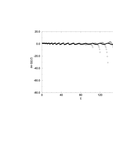
Figure 2: ${\mathcal{I}}m\{G(t,t^{\prime})\}$ : Chebyshev/exact result (filled) versus the finite-difference result corresponding to the trapezoidal method (empty).

In Figs. 1 and 2 we compare the exact result and the finite-difference result corresponding to the trapezoidal method for a case when the problem has a closed-form solution. We choose

$$Q(t,t^{\prime}) = -\sin(t-t^{\prime})+{\rm i}\cos(t-t^{\prime})\>,$$

$$G_{0}(t,t^{\prime}) = (t-t^{\prime})\cos(t-t^{\prime})$$

$$+{\rm i}[\cos(t-t^{\prime})-(t+t^{\prime})\sin(t-t^{\prime})]\>,$$

$$G(t,t^{\prime}) = \sin(t-t^{\prime})+{\rm i}\cos(t-t^{\prime})\>.$$

As we are interested only in the values of $G(t,t^{\prime})$ for $t^{\prime}\leq t$, we depict the real and imaginary parts of $G(t,t^{\prime})$ as a function of the band index $\tau=i(i-1)/2+j$, with $j\leq i$, used to store the lower half of the matrix. Given the domain $0\leq t\leq 6$ and the same number of grid points ($N$=16), the result obtained using the Chebyshev expansion approach can not be visually distinguished from the exact result, i.e. the absolute value of the error at each grid point is less than $10^{-5}$. As expected we also see that the errors made on ${\mathcal{I}}m\{G(t,t^{\prime})\}$ by using the finite-difference method are a lot worse than the errors on ${\mathcal{R}}e\{G(t,t^{\prime})\}$. As pointed out before, this is due to the fact that the equation for ${\mathcal{R}}e\{G(t,t^{\prime})\}$ is independent of any prior knowledge of ${\mathcal{I}}m\{G(t,t^{\prime})\}$ while we determine ${\mathcal{I}}m\{G(t,t^{\prime})\}$ based on the approximation of ${\mathcal{R}}e\{G(t,t^{\prime})\}$.

IV Boundary value problem

In principle, the course of action taken in the previous section, namely converting a differential equation into an integral equation, also works in the context of a boundary value problem. Let us consider the second-order ordinary differential equation

$$y^{\prime\prime}(x)\ +\ f[y^{\prime}(x),y(x),x]\ =\ 0\>,\quad x\in[a,b]\>,$$ (27)

with the boundary conditions

$$g[y(a),y^{\prime}(a)]=c_{a}\>,\quad h[y(b),y^{\prime}(b)]=c_{b}\>.$$ (28)

No restriction on the actual form of the function $f[y^{\prime}(x),y(x),x]$ is implied, so both linear and nonlinear equations are included.

We integrate Eq. (27) to obtain

$$y^{\prime}(x)-y^{\prime}(a)+\int_{a}^{x}f[y^{\prime}(x^{\prime}),y(x^{\prime}),x^{\prime}]\,{\rm d}x^{\prime}\ =\ 0\>.$$ (29)

A second integration gives

$$y(x)-y(a)-(x-a)y^{\prime}(a)$$

$$+\int_{a}^{x}\ \int_{a}^{x^{\prime}}f[y^{\prime}(x^{\prime\prime}),y(x^{\prime\prime}),x^{\prime\prime}]\,{\rm d}x^{\prime\prime}\,{\rm d}x^{\prime}\ =\ 0\>.$$ (30)

The last equation is equivalent to Eq. (19). However, for an initial value problem, the values of $y(a)$ and $y^{\prime}(a)$ are readily available. In order to introduce the boundary conditions for a boundary value problem, we must consider first a separate system of equations for $y(a)$, $y(b)$, $y^{\prime}(a)$ and $y^{\prime}(b)$, which is obtained by specializing Eqs. (29) and (30) for $x=b$, together with the boundary conditions given in (28). Then one can proceed with solving Eq. (30) using the techniques presented in the previous section. For instance, the Dirichlet problem

$$y(a)\ =\ y(b)\ =\ 0\>,$$ (31)

leads to the integral equation

$$y(x)+\left\{\frac{x-a}{b-a}\int_{a}^{b}+\int_{a}^{x}\right\}\$$ (32)

$$\times\int_{a}^{x^{\prime}}f[y^{\prime}(x^{\prime\prime}),y(x^{\prime\prime}),x^{\prime\prime}]\,{\rm d}x^{\prime\prime}\,{\rm d}x^{\prime}\ =\ 0\>.$$

Note, that one can also double the number of unknowns and solve Eqs. (29) and (30) simultaneously for $y(x)$ and $y^{\prime}(x)$.

In this section however, we will discuss boundary value problems from the perspective of a perturbative approach, where we start with an initial guess of the solution $y_{0}$ that satisfies the boundary conditions of the problem, and write $y=y_{0}+\epsilon$, with $\epsilon$ being a variation obeying null boundary conditions. We then solve for the perturbation $\epsilon$ such that the boundary values remain unchanged. This approach allows us to treat linear and nonlinear problems on the same footing, and avoids the additional complications regarding boundary conditions.

We assume that $y_{0}(x)$ is an approximation of the solution $y(x)$ satisfying the boundary conditions (28). Then we can write

$$y(x)\ =\ y_{0}(x)\ +\ \epsilon(x)\>,$$

where the variation $\epsilon(x)$ satisfies the boundary conditions

$$g[\epsilon(a),\epsilon^{\prime}(a)]=0\>,\quad h[\epsilon(b),\epsilon^{\prime}(b)]=0\>.$$

We now use the Taylor expansion of $f[y^{\prime}(x),y(x),x]$ about $y(x)=y_{0}(x)$ and keep only the linear terms in $\epsilon(x)$ and $\epsilon^{\prime}(x)$ to obtain an equation for the variation $\epsilon(x)$

$$\epsilon^{\prime\prime}(x)\,+\,\left.\frac{\partial f[y^{\prime}(x),y(x),x]}{\partial y^{\prime}(x)}\right|_{y(x)=y_{0}(x)}\epsilon^{\prime}(x)$$ (33)

$$\,+\,\left.\frac{\partial f[y^{\prime}(x),y(x),x]}{\partial y(x)}\right|_{y(x)=y_{0}(x)}\epsilon(x)$$

$$\,=\,\,-\,y_{0}^{\prime\prime}(x)\,-\,f[y_{0}^{\prime}(x),y_{0}(x),x]\>.$$

Equation (33) is of the general form (17)

$$\epsilon^{\prime\prime}(x)\ +\ p(x)\,\epsilon^{\prime}(x)\ +\ q(x)\,\epsilon(x)\ =\ r(x)\>,$$

with

$$p(x) = \left.\frac{\partial f[y^{\prime}(x),y(x),x]}{\partial y^{\prime}(x)}\right|_{y(x)=y_{0}(x)}\>,$$

$$q(x) = \left.\frac{\partial f[y^{\prime}(x),y(x),x]}{\partial y(x)}\right|_{y(x)=y_{0}(x)}\>,$$

$$r(x) = -\ y_{0}^{\prime\prime}(x)\ -\ f[y_{0}^{\prime}(x),y_{0}(x),x]\>.$$

Using the Chebyshev representation of the derivatives, Eqs. (9, 10), and depending on the grid used, we solve a system of linear equations (20) for the perturbation function $\epsilon(x)$. The elements of the matrices $A$ and $C$ are given as

$$A_{ij} = [D^{2}]_{i\,j}\ +\ p(x_{i})\,D_{i\,j}\ +\ q(x_{i})\,\delta_{i\,j}\>,$$

$$C_{i} = r(x_{i})\>,\quad i,j=1,2,\ldots,N\>,$$

for the grid (1), and

$$A_{ij} = [\tilde{D}^{2}]_{i\,j}\ +\ p(\tilde{x}_{i})\,\tilde{D}_{i\,j}\ +\ q(\tilde{x}_{i})\,\delta_{i\,j}\>,$$

$$C_{i} = r(\tilde{x}_{i})\>,\quad i,j=1,\ldots,N-1\>,$$

for the grid (2).

The iterative numerical procedure is straightforward: Starting out with an initial guess $y_{0}(x)$ we solve Eq. (33) for the variation $\epsilon(x)$; then we calculate the new approximation of the solution

$$y_{0}^{\rm new}\ =\ y_{0}^{\rm old}\ +\ \epsilon(x)\>,$$ (34)

and repeat the procedure until the difference $\epsilon(x)$ gets smaller than a certain $\varepsilon$ for all $x$ at the grid points.

It is interesting to notice that this approach can work even if the solution is not differentiable at every point of the interval where it is defined (Gibbs phenomenon), provided that the lateral derivatives are finite. As an example, let us consider the case of the equation

$$x\,y^{\prime}(x)\ -\ y(x)\ =\ 0\>,$$ (35)

which has the solution $y(x)=|x|$. In Fig. 3 we compare the numerical solutions for different values of $N$ on the interval $[-1,1]$. We see that for $N=64$ the numerical solution can not be visually discerned from the exact solution. Eq. (35) is a good example of a situation when it is desirable to use an even, rather than an odd, number of grid points, in order to avoid any direct calculation at the place where the first derivative $y^{\prime}(x)$ is not continuous.

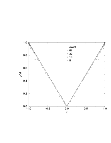
Figure 3: Numerical solutions of Eq. (35) obtained for different values of $N$, using the Chebyshev expansion approach; we chose $y_{0}(x)=x^{2}$, for $-1\leq x\leq 1$

We apply the perturbation approach outlined above to a couple of singular, nonlinear second-order boundary value problems arising in fluid dynamics. The first example ref:john_1a

$$y^{\prime\prime}(x)\ +\ \frac{\phi(x)}{y^{\lambda}(x)}\ =\ 0\>,\quad\lambda>0\>,$$ (36)

gives the Emden-Fowler equation when $\lambda$ is negative. In order to solve Eq. (36), we introduce the variation $\epsilon(x)$ as a solution of the equation

$$\epsilon^{\prime\prime}(x)\ -\ \lambda\,\frac{\phi(x)}{y_{0}^{\lambda+1}(x)}\ \epsilon(x)\ =\ -\ \left\{y_{0}^{\prime\prime}(x)+\frac{\phi(x)}{y_{0}^{\lambda}(x)}\right\}\>.$$

The second example we consider is similar to a particular reduction of the Navier-Stokes equations ref:john_2

$$y^{\prime\prime}(x)\ -\ \frac{\phi(x)}{y^{2}(x)}\ y^{\prime}(x)\ =\ 0\>.$$ (37)

In this case, the variation $\epsilon(x)$ is a solution of the equation

$$\epsilon^{\prime\prime}(x)\ -\ \frac{\phi(x)}{y_{0}^{2}(x)}\,\epsilon^{\prime}(x)\ +\ 2\frac{\phi(x)}{y_{0}^{3}(x)}\,y_{0}^{\prime}(x)\ \epsilon(x)$$

$$\ =\ -\ \left\{y_{0}^{\prime\prime}(x)-\frac{\phi(x)}{y_{0}^{2}(x)}\,y^{\prime}(x)\right\}\>.$$

In both cases we are seeking solutions $y(x)$ on the interval $[0,1]$, corresponding to the boundary conditions

$$y(0)\ =\ y(1)\ =\ 0\>.$$ (38)

Then, we choose $y_{0}(x)=\sin(\pi x)$ as our initial approximation of the solution. Given the boundary values (38), we see that the function $f[y^{\prime}(x),y(x),x]$ exhibits singularities at both ends of the interval $[0,1]$. However, since the variation $\epsilon(x)$ satisfies null boundary conditions, we avoid the calculation of any of the coefficients at the singular points no matter which of the grids (1, 2) we choose. We consider the case when the above problems have the closed-form solution $y(x)=x(1-x)$, with $\lambda=1/2$ in Eq. (36). In Fig. 4 we compare the exact result with the numerical solutions obtained using the Chebyshev expansion corresponding to the grid (1).

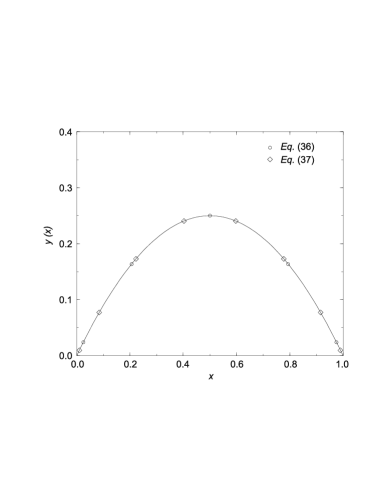
Figure 4: Chebyshev/exact solution of Eqs. (36) and (37) versus numerical solutions obtained using the Chebyshev expansion approach.

The last example we consider arises in the study of ocean currents, specifically the mathematical explanation of the formation of currents like the Gulf Stream. Then, one has to solve a partial differential equation of the type

$$\left[\frac{\partial^{2}}{\partial x^{2}}\ +\ \frac{\partial^{2}}{\partial y^{2}}\ +\ a(x,y)\,\frac{\partial}{\partial x}\right]\,u(x,y)\ =\ g(x,y)\>,$$ (39)

subject to null boundary conditions. To illustrate how the method works in two dimensions, we consider the case of a known solution $u(x,y)=\sin(\pi x)*\sin(\pi y)$, defined on a square domain $[0,1]\times[0,1]$ with $a(x,y)=1$, and compare the results obtained via a Chebyshev expansion versus the results obtained via a finite-difference technique. We choose the function $u_{0}(x,y)=xy(1-x)(1-y)$ as our initial guess. In Fig. 5 we plot the exact result versus the finite-difference result corresponding to the same number of points ($n_{x}=n_{y}=N$=8) for which the proposed Chebyshev expansion approach is not distinguishable from the exact result. The number of iterations necessary to achieve the desired accuracy is very small (typically one iteration is enough!), while the finite-difference results are obtained after 88 iterations.

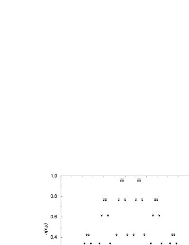
Figure 5: Chebyshev/exact solution (filled) of Eq. (39) versus the finite-difference result (empty) obtained for $N=8$, as a function of the band index $\tau=(i-1)N+j$.

Of course, the grid can be refined by using a larger number of mesh points. Then, the number of iterations increases linearly for the finite-difference method, while the number of iterations necessary when using the Chebyshev expansion stays pretty much constant. In general, we do not expect that by using the Chebyshev expansion, we will always be able to obtain the desired result after only one iteration. However, the number of necessary iterations is comparably very small and does not depend dramatically on the number of grid points. This can be a considerable advantage when we use a large number of grid points and want to keep the computation time to a minimum.

V Conclusions

We have presented practical approaches to the numerical solutions of initial value and second-order boundary value problems defined on finite domains, based on a spectral method known as El-gendi’s method. The method is quite general and has some special advantages for certain classes of problems. This method can be used also as an initial test to scout the character of the solution. Failure of the Chebyshev expansion method presented here should tell us that the solution we seek can not be represented as a polynomial of order $N$ on the considered domain.

The Chebyshev grids (1) and (2) provide equally robust ways of discretizing a continuous problem, the grid (1) allowing one to avoid the calculation of functions at the ends of the interval, when the equations have singularities at these points. The fact that the proposed grids are not uniform should not be considered by any means as a negative aspect of the method, since the grid can be refined as much as needed. The numerical solution in between grid points can always be obtained by interpolation. The Chebyshev grids have the additional advantage of being optimal for the cubic spline interpolation scheme ref:spline .

The Chebyshev expansion provides a robust method of computing the integral and derivative of a non-singular function defined on a finite domain. For example, if both the solution of an initial value problem and its derivative are of interest, it is better to transform the differential equation into an integral equation and use the values of the function at the grid points to also compute the value of the derivative at these points.

Figure 6: Standard deviation of the approximation for ${\mathcal{R}}e\{G(t,t^{\prime})\}$ as a function of the number of grid sites: Chebyshev (filled) and finite-difference (empty) results.

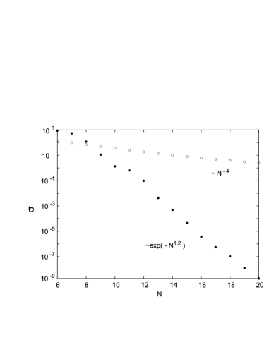
Figure 7: Standard deviation of the approximation for ${\mathcal{I}}m\{G(t,t^{\prime})\}$ as a function of the number of grid sites: Chebyshev (filled) and finite-difference (empty) results.

Figure 8: Standard deviation of the approximation for the solution of Eq. (39) versus the number of mesh sites $n_{x}n_{y}=N^{2}$: Chebyshev (filled) and finite-difference (empty) results.

It is a well-known fact that spectral methods are more expensive that finite-differences for a given grid size, so in order to reach some specified accuracy there is always a tradeoff: finite differences need more points, but are cheaper per point. The goal is to reach a certain numerical accuracy requirement as efficiently as possible. Therefore let us discuss here some computational cost considerations for sample calculations. We shall comment on two of the calculations presented in this paper: the calculation for the $G(t,t^{\prime})$ (see Eq. (22)) and the solution of Eq. (39). In Figs. 6, 7 and 8 we depict the convergence of the finite-difference and Chebyshev methods for obtaining the approximate solutions, and we illustrate the elapsed computer time in Figs. 9 and 10. The error of the Chebyshev expansion method decays exponentially as a function of $N$, while the error of the finite-difference method can be expressed as a power of $N$. For both methods, the running time depends exponentially of $N$. We conclude that indeed the execution time required by the spectral method increases faster with the number of grid points than the finite-difference method. However, in order to achieve a reasonable accuracy (e.g. $\sigma<10^{-6}$), the Chebyshev method requires only a small grid, and for this small number of grid points the computer time is actually modest. All calculations where carried out on a (rather old) Pentium II 266 MHz PC. There were no additional numerical algorithms required for performing the finite-difference calculation, as these involve simple iterations of the initial guess. Due to the global character of the Chebyshev calculation, one needs to solve a system of linear equations. Since this is a sparse system of equations we have employed an iterative biconjugate gradient method ref:nr for obtaining the numerical solution. For both problems, the sparsity of the relevant matrices is $\sim 2/N$.

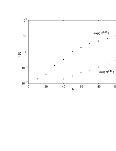
Figure 9: Execution time for obtaining an approximation for $G(t,t^{\prime})$ as a function of the number of grid sites: Chebyshev (filled) and finite-difference (empty) results.

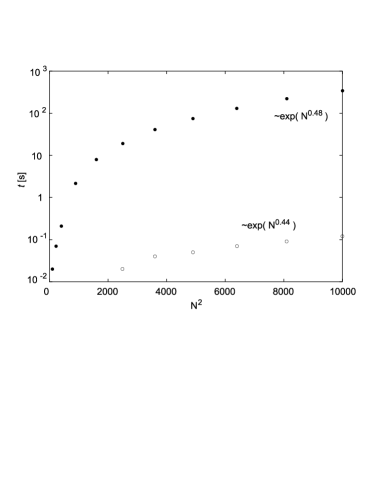
Figure 10: Execution time for obtaining an approximate solution of Eq. (39) versus the number of mesh sites $n_{x}n_{y}=N^{2}$: Chebyshev (filled) and finite-difference (empty) results.

Most importantly, we have shown that the Chebyshev expansion is applicable to efficiently solving complex nonlinear integral equations of the form encountered in a Schwinger-Dyson approach to determining the time evolution of the unequal time correlation functions of non-equilibrium quantum field theory. In this particular context, spectral methods have made possible for the first time to carry out complex dynamical calculations at next to leading order in quantum mechanics and field theory. Our results will form the basis for future studies of quantum phase transitions.

References

- (1) Kerman A K and Koonin S E 1976 Ann. Phys. 100 332 Jackiw R and Kerman A K 1979 Phys. Lett. A 71 158 Guth A H and Pi S-Y 1985 Phys. Rev. D 32 1899 Cooper F, Pi S-Y, and Stancioff P 1986 Phys. Rev. D 34 3831 Pi S-Y and Samiullah M 1987 Phys. Rev. D 36 3128
- (2) Boyanovsky D and de Vega H J 1993 Phys. Rev. D 47 2343 Boyanovsky D, de Vega H J, Holman R, Lee D-S, and Singh A 1995 Phys. Rev. D 51 4419 Boyanovsky D, de Vega H J, Holman R, and Salgado J 1996 Phys. Rev. D 54 7570 Boyanovsky D, Cormier D, de Vega H J, Holman R, Singh A, and Srednicki M 1997 Phys. Rev. D 56 1939 Boyanovsky D, D’Attanasio M, de Vega H J, Holman R, and Lee D-S 1995 Phys. Rev. D 52 6805 Vautherin D and Matsui T 1997 Phys. Rev. D 55 4492 Boyanovsky D, de Vega H J, Holman R, and Salgado J 1998 Phys. Rev. D 57 7388
- (3) Cooper F and Mottola E 1987 Phys. Rev. D 36 3114 Cooper F, Kluger Y, Mottola E, and Paz J P 1995 Phys. Rev. D 51 2377 Kluger Y, Cooper F, Mottola E, Paz J P, and Kovner A 1995 Nucl. Phys. A 590 581c Lampert M A, Dawson J F, and Cooper F 1996 Phys. Rev. D 54 2213 Cooper F, Kluger Y, and Mottola E 1996 Phys. Rev. C 54 3298
- (4) Wetterich C 1997 Phys. Rev. Lett. 78 3598 Bettencourt L and Wetterich C 1998 Phys. Lett. B 430 140 Bonini G F and Wetterich C 1999 Phys. Rev. D 60 105026
- (5) Aarts G, Bonini G F, and Wetterich C 2001 Phys. Rev. D 63 025012
- (6) Cooper F, Habib S, Kluger Y, Mottola E, Paz J, and Anderson P 1994 Phys. Rev. D 50 2848 Cooper F, Dawson J F, Habib S, Kluger Y, Meredith D, and Shepard H 1995 Physica D 83 74
- (7) Berges J and Cox J 2001 Phys. Lett. B 517 369 Berges J 2001 Controlled nonperturative dynamics of quantum fields out of equilibrium Nucl. Phys. A (in press)
- (8) Clenshaw C W and Curtis A R 1960 Numer. Math. 2 197 Imhof J P 1963 Numer. Math. 5 138
- (9) Elliott D 1965 Math. Comp. 19 234 Fraser W and Wilson M W 1996 SIAM Rev. 8 322
- (10) Press W H, Teukolsky S A, Vetterling W T, and Flannery B P 1992 Numerical Recipes in FORTRAN : the art of scientific computing, (New York: Cambridge University Press)
- (11) Fox L 1962 Comput. J. (UK) 4 318 Clenshaw C W and Norton H J 1963 Comput. J. (UK) 6 88
- (12) Elliott D 1963 Comput. J. (UK) 6 102
- (13) Boyd J P 1989 Chebyshev and Fourier Spectral Methods, (New York: Springer Verlag) Canuto C, Hussaini M Y, Quarteroni A, and Zang T A 1988 Spectral Methods for Fluid Dynamic, (New York: Springer Verlag) Fornberg B 1996 A Practical Guide to Pseudospectral Methods, (New York: Cambridge University Press) Funaro D 1997 Spectral Elements for Transport-Dominated Equation, vol 1 of Lectures Notes in Computational Science and Engineering, (Heidelberg: Springer Verlag) Gottlieb D and Orszag S A 1977 Numerical Analysis of Spectral Methods, (Philadelphia: SIAM) Gottlieb D, Hussaini M Y, and Orszag S A 1984 Theory and application of spectral methods, in Spectral Methods for Partial Differential Equations (ed R G Voigt, D Gottlieb, and M Y Hussainni) (Philadelphia: SIAM) p 1
- (14) El-gendi S E 1969 Comput. J. (UK) 12 282
- (15) Delves L M and Mohamed J L 1985 Computational Methods for Integral Equations, (Cambridge: Cambridge University Press)
- (16) Mihaila B, Dawson J F, and Cooper F 1997 Phys. Rev. D 56 5400 Mihaila B, Athan T, Cooper F, Dawson J F, and Habib S 2000 Phys. Rev. D 62 125015 Mihaila B, Dawson J F, and Cooper F 2001 Phys. Rev. D 63 096003
- (17) Blagoev K, Dawson J F, Cooper F, and Mihaila B 2001 Schwinger-Dyson approach to non-equilibrium classical field theory Phys. Rev. D (in press)
- (18) Schwinger J 1961 J. Math. Phys. 2 407 Bakshi P M and Mahanthappa K T 1963 J. Math. Phys. 4 1 ;ibid. J. Math. Phys. 4 12 Keldysh L V 1964 Zh. Eksp. Teo. Fiz. 47 1515 [Sov. Phys. JETP 20 (1965) 1018]
- (19) Taliaferro S 1979 Nonlinear Anal. Theory Methods Appl. 3 897 Baxley J V 1991 SIAM J. Math. Anal. 22 463
- (20) Baxley J V 1997 private communication
- (21) deBoor C 1978 A Practical Guide to Splines, (New York: Springer-Verlag)