Millisecond and Binary Pulsars as Nature’s Frequency Standards.
III. Fourier Analysis and Spectral Sensitivity of Timing Observations to Low-Frequency Noise

Abstract

Millisecond and binary pulsars are the most stable natural frequency standards which admits to introduce modified versions of universal and ephemeris time scales based correspondingly on the intrinsic rotation of pulsar and on its orbital motion around barycenter of a binary system. Measured stability of these time scales depends on numerous physical phenomena which affect rotational and orbital motion of the pulsar and observer on the Earth, perturb propagation of electromagnetic pulses from pulsar to the observer and bring about random fluctuations in the rate of atomic clock used as a primary time reference in timing observations. On the long time intervals the main reason for the instability of the pulsar time scales is the presence of correlated, low-frequency timing noise in residuals of times of arrivals (TOA) of pulses from the pulsar which has both astrophysical and geophysical origin. Hence, the timing noise can carry out the important physical information about interstellar medium, interior structure of the pulsar, stochastic gravitational waves coming from the early universe, etc. Each specific type of the low-frequency noise can be described in framework of power law spectrum model. Although the data processing of pulsar timing observations in time domain seems to be the most imformative it is significantly important to know to which spectral bands single and binary pulsars, considered as detectors of the low-frequency noise signal, are the most sensitive. Solution of this problem may be reached only if a parallel processing of timing data in frequency domain is fulfilled. This requires a development of the Fourier analysis technique for an adequate interpretation of data contaminated by the correlated noise with a singular spectrum. The given problem is examined in the present article.

1 Introduction

Millisecond and binary pulsars are known as exellent probes for testing theory of general relativity Taylor & Weisberg 1982, 1989), structure of interstellar medium (Rickett 1990, 1996) and interior of neutron stars (Cordes & Greenstein 1981, Kaspi et al. 1994) as well as setting upper limit on the energy density of primordial gravitational radiation (Kaspi , Thorsett & Dewey 1996, McHugh et al. 1997, Kopeikin 1997a, Kopeikin & Wex 1999). Rotational motion of a pulsar around its own axis had been proposed (Shabanova et al. 1979, Backer et al. 1982, Rawley et al. 1987, Matsakis et al. 1997) for using as a new time reference being analogue of universal time in astrometry. Quite recently, a new step toward to estiblishing a stable time scale on extremely long intervals approaching 50-100 years has been suggested (Ilyasov et al. 1998, Kopeikin 1999). It is extracted from the orbital motion of pulsar in a binary system and represents the analogue of ephemeris time of classical astronomy introduced by Newcomb (1898)at the end of last century and based on the orbital motion of the Earth around the Sun.

An adequate analysis of timing data requires deeper understanding of nature of a noise process dominating in pulsar timing residuals. As soon as the autocovariance function of the noise process is known the analysis in time domain becomes possible. Time domain analysis is the most informative since the observed stochastic process is not usually stationary and includes the non-stationary component as well (Groth 1975, Cordes 1978, 1980; Kopeikin 1997b). Because pulsar timing observations are conducted on relatively long time intervals the white noise of errors in measuring TOA of pulsar’s pulses will be suppressed by the presence of a number of correlated, low-frequency (red) noises having different spectra and intencities. Henceforth, we are mainly interested in analysing the red noise.

The simple model of such noise has been worked out by one of us (Kopeikin 1997b). It is based on the shot noise approximation and do includes a dependence of the autocovariance function on both stationary and non-stationary components of red noise. In the process of elaborating the given model a rather remarkable fact has been established (Kopeikin 1999), namely, that timing residuals and variances of some spin-down and all orbital parameters are not affected by the non-stationary component of the red noise at all. This discovery put on a firm ground the Fourier analysis of TOA residuals and variances of fitting parameters in frequency domain. This analysis gives exhaustive information about the noise process itself and admits us to reveal to which frequency harmonics in the spoectral expansion of the stochastic process pulsar timing observations are the most sensitive. Moreover, just we have an adequate approach for the treatment of red noise in frequency domain a lot of interesting applications is opened having the goal to study the physical nature of the low frequency noises with arbitrary spectrum.

Any low-frequency noise can be approximately characterized by the power-law spectrum $S(f)\sim f^{-n}$ where the spectral (integer) index $n\geq 1$. It is obvious that the spectrum has a singularity at zero frequency. Hence, the energy of TOA residuals comprised in such noise should has infinite value because the integral over all frequencies from zero to infinity taken from $S(f)$ is divergent. Clearly, this has no physical meaning and one has to resort to special mathematical tricks in order to avoid this artificial divergency. There are two ways for curing this flaw. First of them consists in analytical continuation of the spectrum by changing it from $S(f)\sim f^{-n}$ to $S(f,A)\sim f^{-(n+A)}$ where $A$ is the pure complex parameter being differnt from zero. Such model of the analitically continued spectrum gives convergent integrals which coincide everywhere on real axis with ones taken from the spectrum $S(f)\sim f^{-n}$ exept for the point $f=0$. In order to prescribe a physical meaning to such integrals we have to expand them in the Laurent series with respect to the parameter A and to take the finite part of the expansion. Such procedure has been used, in particular, by Kopeikin (1997a) for calculation of autocovariance function of stochastic noise of the primordial gravitational wave background having spectrum $S(f)\sim f^{-5}$ (Mashhoon 1982, 1985, Mashhoon & Seitz 1991, Bertotti et al. 1983).

The procedure of analytical continuation of divergent inetgrals is mathematically rigorous and theoretically powerful tool which gives well-defined and self-consistent results (Gel’fand & Shilov 1964). However, it is inconvinuent for people doing numerical computations. For them, the second method of regularization of singular spectra seems to be more preferable and practically useful. It is based on the truncation of all divergent integrals at the lower cut-off frequency $f=\varepsilon$ along with corresponding modification of the power-law model of the red noise spectrum in order to avoid the model dependence of results of fitting procedure on the artificially introduced cut-off frequency. It will be shown that the simplest way of modification of the spectrum can be reduced to the addition to the existing power-law spectrum of red noise of the infinite sum consisting of the Dirac delta function and its derivatives having local support at the lower cut-off frequency $f=\varepsilon$. Such modernization of the spectrum preserves the structure of the autocovariance function and, as a consequence, do not vilolate results of numerical computations in time domain. This second method of regulariazation of divergent integrals will be used in the present paper.

In what follows it is more convinuent for us to work in terms of dimensionless frequency and time. For instance, in binary pulsars it is preferable for analytic calculations to measure time in units of orbital frequency $n_{b}=2\pi/P_{b}$, where $P_{b}$ is the orbital period of the binary. Then, frequency $f$ is measured in units of $1/P_{b}$ and dimensionless time is the pulsar’s mean anomaly $u=n_{b}\tau$. Hereafter, we use $u$ instead of $\tau$.

2 Regularized Spectrum of Low-Frequency Noise

Any gaussian low-frequency noise is completely characterized by the autocovariance function which describes correlation between two values of stochastic process separated by the arbitrary time interval $\tau=t_{2}-t_{1}$. Autocovariance function consists usually of two algebraically independent parts characterizing separately stationary $R^{-}(\tau)$ and non-stationary $R^{+}(\tau)$ components of the noise. Complete expressions of autocovariance functions for different events of low-frequency noise have been derived in the paper (Kopeikin 1997b) where the shot noise approximation of stochastic process has been used. Although both stationary and non-stationary components of autocovariance function are important for an adequate treatment of observations (Kopeikin 1999) we are dealing in the present paper only with the stationary part which posseses to be transformed into the spectral density of noise $S(f)$ by means of the Wiener-Khintchine theorem

$$R^{-}(u)=2\int_{0}^{\infty}S(f)\cos(2\pi fu)df.$$ (1)

If (constant) intensity of noise is denoted by $h_{n}$ then autocovariance function of low-frequency correlated noise is determined by the expression (Kopeikin 1997b)

$$\left\{\begin{array}[]{ll}C_{n}h_{n}|u|^{n-1},&\mbox{$n=2,4,6,...$, random walk noise}\\ \\ C_{n}h_{n}u^{n-1}\ln|u|,&\mbox{$n=1,3,5,...$, flicker noise}\end{array}\right.$$ (2)

where $C_{n}$ is a numerical constant of normalization.

Functions, which might be appropriate candidates for the spectrum of noise procesess with the foregoing autocovariance functions, are $S(f)={\rm const}f^{-n}$ where $n$ is integer. However, integrals (1) from such power-law functions are divergent because of non-physical singularity at zero frequency. For this reason, regularization technique should be used because we don’t know usually the low-frequency behavior of the spectrum.

2.1 Analaitic Continuation Technique

Analytic continuation regularization procedure is contained in that one extends the spectrum $S(f)$ in the complex plane domain by introducing the function

$$S(f,A)={\rm const}f^{-n-A}$$ (3)

where $A$ is a complex parameter. Autocovariance function becomes an analytically continued functional of the complex variable $A$:

$$R^{-}(u,A)=2\int_{0}^{\infty}S(f,A)\cos(2\pi fu)df,$$ (4)

which coincides (due to the properties of analytically continued complex functions) exactly with the integral in (1) exept at the point $A=0$. The functional (4) with the spectrum defined by eq. (3) is a table integral and can be easily calculated analitically. After calculation of the integral it is expanded in the Laurent series near the point $A=0$. It yields

$$R^{-}(u,A)=\frac{1}{A}{\rm Residue}_{A=0}\left\{R^{-}(u,A)\right\}+R^{-}(u,A=0)+...\quad.$$ (5)

The first term in the expansion is a simple pole with respect to $A$. The second term in the expansion is finite and gives exactly the autocovariance function given in eq. (2). Regularization of the integral (4) means that we take only its finite part and abandon the singular term. Analytic continuation technique is powerful theoretical tool (Kopeikin 1997a) but it hardly can be used in numerical computations for which infrared cut-off technique is much better.

2.2 Infrared Cut-off Technique

The power spectrum $S(f)$ of the noise is defined using the truncated Fourier transform with the lower cut-off frequency $f=\varepsilon$. Namely, we require that the truncated cosine Fourier transform of $S(f)$ must give the stationary part of the original autocovariance function (2) without any additional contributions. Let us postulate that the spectrum $S(f)$ may be represented by the formula

$$S(f)=\left\{\begin{array}[]{ll}h_{n}\left[\displaystyle{\frac{1}{(2\pi f)^{n}}}+\displaystyle{\sum_{k=0}^{\infty}}B_{2k}(\varepsilon)\varepsilon^{2k}\delta^{(2k)}(f-\varepsilon)\right],&\mbox{if $f\geq\varepsilon$}\\ \\ 0,&\mbox{otherwise}\end{array}\right.$$ (6)

where the spectral index of noise $n=1,2,...,6$, constant parameter $h_{n}$ is the strength of noise, quantities $B_{k}(\varepsilon)$ are constant numerical coefficients being defined later, and $\delta^{(k)}(f-\varepsilon)$ denotes the $n-th$ derivative with respect to $f$ of the Dirac delta-function $\delta(f-\varepsilon)$. The Dirac delta function is defined according to the condition (Korn & Korn 1968)

$${\int_{a}^{b}f(x)\delta(x-X)dx}=\left\{\begin{array}[]{ll}0,&\mbox{if $X<a$, or $X>b$,}\\ \\ \frac{1}{2}f(X+0),&\mbox{if $X=a$,}\\ \\ \frac{1}{2}f(X-0),&\mbox{if $X=b$,}\\ \\ \frac{1}{2}\left[f(X-0)+f(X+0)\right],&\mbox{if $a<X<b$,}\end{array}\right.$$ (7)

where $f(x)$ is arbitrary function being such that unilateral limits $f(X-0)$ and $f(X+0)$ exist. Coefficients $B_{k}(\varepsilon)$ are determined by the condition that the cosine Fourier transform of $S(f)$ gives stationary part of autocovariance function of corresponding low-frequency noise the model of which may be found in papers (Kopeikin 1997b, 1999). As an example of derivation of $B_{k}(\varepsilon)$ we determine the several first coefficients $B_{k}(\varepsilon)$ in the event of flicker noise in pulsar’s rotational phase which has the spectral index $n=1$. Coefficients $B_{k}(\varepsilon)$ for noises having other spectral indices will be displayed in this section without proof which is rather straightforward.

Stationary part of autocovariance function $R^{-}(\tau)$ of flicker noise in pulsar’s phase is equal to $h_{1}\pi^{-1}\log|u|$. According to definition of the spectrum we should have

$$R^{-}(u)=2\displaystyle{\int_{\varepsilon}^{\infty}}S(f)\cos(2\pi fu)df.$$ (8)

Substituting $S(f)$ from Eq. (6) with $n=1$ to right hand side of Eq. (8) and taking integrals we get

$$R^{-}(u)=-\frac{h_{1}}{\pi}{\bf Ci}(2\pi\varepsilon|u|)+h_{1}\cos(2\pi\varepsilon u)\displaystyle{\sum_{k=0}^{\infty}}(-1)^{k}B_{2k}(\varepsilon)(2\pi\varepsilon u)^{2k},$$ (9)

where ${\bf Ci}(x)$ is the cosine integral, and we have used the formula (Korn & Korn 1968)

$$2\displaystyle{\int_{\varepsilon}^{\infty}}\delta^{(2k)}(f-\varepsilon)\cos(2\pi fu)df=\frac{d^{2k}}{d\varepsilon^{2k}}\cos(2\pi\varepsilon u)=(-1)^{k}(2\pi u)^{2k}\cos(2\pi\varepsilon u)$$ (10)

Taylor expansion of the cosine integral and $\cos(2\pi\varepsilon u)$ in the right hand side of the expression (9) with respect to small parameter $\varepsilon$ yields

$$R^{-}(u)=\frac{h_{1}}{\pi}\left[-\log|u|-\gamma-\log(2\pi\varepsilon)\right]+h_{1}\biggl{\{}B_{0}(\varepsilon)+(2\pi\varepsilon u)^{2}\left[\frac{1}{2\pi}-\frac{1}{2}B_{0}(\varepsilon)-B_{2}(\varepsilon)\right]\biggr{\}}+O(\varepsilon^{4}).$$ (11)

Since $R^{-}(u)$ must be equal to $-h_{1}\pi^{-1}\log|u|$, we find from Eq. (11)

$$B_{0}(\varepsilon)=\frac{\gamma}{\pi}+\frac{c\log(2\pi\varepsilon)}{\pi},\hskip 56.9055ptB_{2}(\varepsilon)=\frac{1}{4\pi}-\frac{\gamma}{2\pi}-\frac{\log(2\pi\varepsilon)}{2\pi}$$ (12)

For practical purposes it is enough to account for the coefficient $B_{0}(\varepsilon)$ only, since all other residual terms appear being multiplied by the factor $2\pi\varepsilon u$ which is negligibly small under the usual circumstances because of smallness of the product $\varepsilon u$. Thus, residual terms are not important as long as the accuracy of observations is not high enough. It is worth emphasizing that the residual terms under discussion are model dependent. Had we chosen another model for the spectrum having slightly another behavior as frequency approaches to zero the residual terms would look differently. These arguments permit to estimate how long we can observe a certain pulsar and process the data with one or another model of red noise spectrum.

Proceeding in the same way for the set of other spectral indeces we obtain the following expressions for the power spectra of low-frequency noises:

1. Flicker noise in phase:

   $$S(f)=\frac{h_{1}}{2\pi}\biggl{\{}\frac{1}{f}+2\left[\gamma+\log(2\pi\varepsilon)\right]\delta(f-\varepsilon)\biggr{\}}+O(\varepsilon^{2}).$$ (13)

2. Random walk in phase:

   $$S(f)=\frac{h_{2}}{4\pi^{2}}\biggl{\{}\frac{1}{f^{2}}-\frac{2}{\varepsilon}\delta(f-\varepsilon)\biggr{\}}+O(\varepsilon).$$ (14)

3. Flicker noise in frequency:

   $$S(f)=\frac{h_{3}}{8\pi^{3}}\biggl{\{}\frac{1}{f^{3}}-\frac{1}{\varepsilon^{2}}\delta(f-\varepsilon)+\left[\log(2\pi\varepsilon)+\gamma-1\right]\delta^{(2)}(f-\varepsilon)\biggr{\}}+O(\varepsilon^{2}).$$ (15)

4. Random walk in frequency:

   $$S(f)=\frac{h_{4}}{16\pi^{4}}\biggl{\{}\frac{1}{f^{4}}-\frac{2}{3\varepsilon^{3}}\delta(f-\varepsilon)-\frac{2}{3\varepsilon}\delta^{(2)}(f-\varepsilon)\biggr{\}}+O(\varepsilon).$$ (16)

5. Flicker noise in frequency derivative:

   $$S(f)=\frac{h_{5}}{32\pi^{5}}\biggl{\{}\frac{1}{f^{5}}-\frac{1}{2\varepsilon^{4}}\delta(f-\varepsilon)-\frac{1}{4\varepsilon^{2}}\delta^{(2)}(f-\varepsilon)+\frac{1}{12}\left[\gamma+\log(2\pi\varepsilon)-\frac{1}{3}\right]\delta^{(4)}(f-\varepsilon)\biggr{\}}+O(\varepsilon^{2}).$$ (17)

6. Random walk in frequency derivative:

   $$S(f)=\frac{h_{6}}{64\pi^{6}}\biggl{\{}\frac{1}{f^{6}}-\frac{2}{5\varepsilon^{5}}\delta(f-\varepsilon)-\frac{2}{15\varepsilon^{3}}\delta^{(2)}(f-\varepsilon)\biggr{\}}+O(\varepsilon).$$ (18)

Let us note that the coefficient $B_{4}(\varepsilon)\equiv 0$ in the expression (18) for spectrum of random walk in frequency derivative.

The expressions given above indicate that there is a strong concentration of infinite energy of the noise at the lower cut-off frequency. As we have stressed already it is a specific feature of the chosen model of the spectrum which appears because we do not know a real behavior of spectrum while frequency is approaching to zero. Another remark is that a direct integration of any of the foregoing spectra with respect to frequency from $f=\varepsilon$ to infinity (which may be erroneosly treated as the energy being stored in TOA residuals) gives zero value which may look surprising. However, it is worth noting that the entire energy presents in TOA residuals can be calculated only after multiplication of the spectrum by the filter function (see section 6 below for more detail). Therefore, calculation of the total energy of residuals is more complicated and always gives a positive numerical value as it should be. Similar arguments can be used in calculating variances of fitting parameters. For example, calculation of variances of the first several spin-down parameters in frequency domain may give a negative numerical value of the variance (Kopeikin 1999) which is physically meaningful. The paradox is solved if we remember about contribution of the non-stationary part of noise which always makes variances of the parameters numerically positive (for more detail see (Kopeikin 1999)).

Pulsar timing observations can be used for estimation of strength and spectrum of low frequency noise presents in TOA residuals. For this reason, development of practically useful estimators of spectrum of noise are required. We are not going to consider in the present paper the question about how to construct the best possible estimators. This subject has been enlightened by a number of other researches (see, for instance, the papers of Deeter & Boynton (1982), Deeter(1984), Taylor 1991, Matsakis al. 1997). Our purpose is to study spectral dependence of TOA residuals and variances of fitting parameters which are used in real practice. In order to make clear what we are doing let us describe, first of all, the timing model we are dealing with.

3 Timing Model

We consider a simplified, but still realistic model of arrival time measurements of pulses from a pulsar in a binary system. It is assumed that the orbit is circular, and the pulsar rotates around its own axis with angular frequency $\nu_{p}$ which slows down due to the electromagnetic (or whatever) energy losses. It is also taken into account that the orbital frequency of the binary system, $n_{b},$ and its projected semimajor axis, $x,$ have a secular drift caused by radial acceleration of the binary (Damour & Taylor 1991, Bell & Bailes 1996), its proper motion of in the sky (Kopeikin 1996), and emission of gravitational waves from the binary (Peters & Mathews 1963, Peters 1964) bringing about the gravitational radiation reaction force (Damour 1983a, Grishchuk & Kopeikin 1983).

The moment ${\cal T}$ of emission of the ${\cal N}$-th pulsar’s pulse relates to the moment $t$ of its arrival measured at the infinite electromagnetic frequency by the equations (Damour & Taylor 1992, Kopeikin 1994, 1999):

$$D\left[{\cal T}+x\sin\left(n_{b}{\cal T}+\sigma\right)\right]=t+\varphi_{0}(t)+\varphi_{1}(t),$$ (19)

$$t=\tau^{\ast}+\Delta_{C}+\Delta_{R\odot}+\Delta_{\pi\odot}+\Delta_{E\odot}+\Delta_{S\odot}.$$ (20)

We use the following notations:

• ${\cal T}$ - pulsar time scale,

• $t$ - barycentric time at the barycenter of the Solar system,

• $\tau^{\ast}$ - topocentric time of observer,

• $\Delta_{C},$ $\Delta_{R\odot},$ $\Delta_{\pi\odot},$ $\Delta_{E\odot},$ $\Delta_{S\odot}$ - clock and astrometric corrections (Taylor & Weisberg 1989, Doroshenko & Kopeikin 1990, 1995) which one assumes to be known precisely,

• $D$ - Doppler factor gradually changing due to the acceleration and proper motion of the binary system in the sky

• $\sigma$ - initial (constant) orbital phase,

• $n_{b}$ - orbital frequency $(n_{b}=2\pi/P_{b})$,

• $i$ - angle of inclination of the orbit to the line of sight,

• $x$ - projected semimajor axis $a_{p}$ of the pulsar’s orbit $(x=a_{p}\sin i/c)$,

• $c$ - speed of light,

• $\varphi_{0}(t)$ - the gaussian noise of TOA measuring errors,

• $\varphi_{1}(t)$ - low-frequency gaussian noise caused by the long-term instabilities of terrestrial clocks, effects in propagation of radio signals in the interstellar medium and stochastic background of primordial gravitational waves, etc.

The rotational phase of the pulsar is given by the polynomial in time

$${\cal N}(t)=\nu_{p}{\cal T}+\frac{1}{2}\stackrel{{\scriptstyle.}}{{\nu}}_{p}{\cal T}^{2}+\frac{1}{6}\stackrel{{\scriptstyle..}}{{\nu}}_{p}{\cal T}^{3}+\frac{1}{24}\stackrel{{\scriptstyle...}}{{\nu}}_{p}{\cal T}^{4}+\frac{1}{120}\stackrel{{\scriptstyle....}}{{\nu}}_{p}{\cal T}^{5}+\nu_{p}\varphi_{2}({\cal T})+O\left({\cal T}^{6}\right),$$ (21)

where $\nu_{p},$ $\stackrel{{\scriptstyle.}}{{\nu}}_{p},\stackrel{{\scriptstyle..}}{{\nu}}_{p},$ etc. are pulsar’s rotational frequency and its time derivatives all referred to the epoch ${\cal T}=0,$ the term $O\left({\cal T}^{6}\right)$ denotes high order derivatives of the rotational phase, and $\varphi_{2}({\cal T})$ is the intrinsic pulsar timing noise in either rotational phase, frequency, or frequency derivative. Solving iteratively equation (19) with respect to ${\cal T}$ and substituting ${\cal T}$ for the right hand side of equation (21) gives a relationship between two observable quantities ${\cal N}$ and $t$:

$${\cal N}(t) = {\cal N}_{0}+\nu t+{\frac{1}{2}}\stackrel{{\scriptstyle.}}{{\nu}}t^{2}+{\frac{1}{6}}\stackrel{{\scriptstyle..}}{{\nu}}t^{3}+{\frac{1}{24}}\stackrel{{\scriptstyle...}}{{\nu}}t^{4}+$$ (22)

$$\mbox{}{\frac{1}{120}}\stackrel{{\scriptstyle....}}{{\nu}}t^{5}-\nu(x+\stackrel{{\scriptstyle.}}{{x}}t+{\frac{1}{2}}\stackrel{{\scriptstyle..}}{{x}}t^{2}+{\frac{1}{6}}\stackrel{{\scriptstyle...}}{{x}}t^{3})\sin(\sigma+n_{b}t+{\frac{1}{2}}\dot{n}_{b}t^{2}+{\frac{1}{6}}\ddot{n}_{b}t^{3})+\nu\epsilon(t),$$

$$\epsilon(t)\stackrel{{\scriptstyle def}}{{=}}\varphi_{0}(t)+\varphi_{1}(t)+\varphi_{2}(t),\vspace{0.3 cm}$$ (23)

where ${\cal N}_{0}$ is the initial rotational phase of the pulsar $({\cal N}_{0}\simeq-\nu t_{0})$; $\nu,$ $\stackrel{{\scriptstyle.}}{{\nu}},$ $\stackrel{{\scriptstyle..}}{{\nu}},...$ are the pulsar’s rotational frequency and its time derivatives at the initial epoch $t_{0};$ $x,$ $\stackrel{{\scriptstyle.}}{{x}},$ $\stackrel{{\scriptstyle..}}{{x}},...$ are the projected semimajor axis of the orbit and its time derivatives at the epoch $t_{0};$ $\sigma,$ $n_{b},$ $\dot{n}_{b},$ $\ddot{n}_{b},...$ are the pulsar’s orbital initial phase, orbital frequency and its time derivatives at the epoch $t_{0}.$ Timing model (22) accounts only for linear terms which is enough for implication of least square method of fitting parameters to the data. All non-linear residual terms of order $x^{2},x\epsilon,$ $\epsilon^{2},$ $\dot{\nu}x$, $\ddot{\nu}x$, etc. are negligible and, for this reason, have been omitted from (22).

We assume that all observations of the binary pulsar are of a similar quality and weight. Then one defines the timing residuals $r(t)$ as a difference between the observed number of the pulse, ${\cal N}^{obs},$ and the number ${\cal N}(t,\theta),$ predicted on the ground of our best guess to the prior unknown parameters of timing model (22), divided by the pulsar’s rotational frequency $\nu$, that is

$$r(t,\theta)=\frac{{\cal N}^{obs}-{\cal N}(t,\theta)}{\nu},\vspace{0.3 cm}$$ (24)

where $\theta=\{\theta_{a},a=1,2,...k\}$ denotes a set of $k$ measured parameters $\left(k=14\mbox{in the model}(\ref{177})\right)$ which are shown in Table 1. It is worth noting that hereafter we use for the reason of convinuence the time argument $u=n_{b}t$, that is the current orbital phase.

Table 1: List of the basic functions and parameters used in the fitting procedure. Spin parameters $\delta{\cal N}_{0},\delta{\nu},\delta\stackrel{{\scriptstyle.}}{{\nu}},\delta\stackrel{{\scriptstyle..}}{{\nu}},\delta\stackrel{{\scriptstyle...}}{{\nu}},\delta\stackrel{{\scriptstyle....}}{{\nu}},$ fit rotational motion of the pulsar around its own axis. Keplerian parameters $\delta{x},\delta\sigma,\delta{n}_{b}$ fit the Keplerian orbital motion of the pulsar about barycentre of the binary system. Post-Keplerian parameters $\delta\stackrel{{\scriptstyle.}}{{x}},\delta\stackrel{{\scriptstyle..}}{{x}},\delta\stackrel{{\scriptstyle...}}{{x}},\delta\stackrel{{\scriptstyle.}}{{n}}_{b},\delta\stackrel{{\scriptstyle..}}{{n}}_{b}$ fit small observable deviations of the pulsar’s orbit from the Keplerian motion caused by the effects of General Relativity, radial acceleartion, and proper motion of barycentre of the binary system with respect to the observer

Parameter			Fitting Function
$\beta_{1}={{\frac{\delta{\cal N}_{0}}{\nu}}}$			$\psi_{1}(t)=1$
$\beta_{2}={\frac{1}{n_{b}}}{{\frac{\delta\nu}{\nu}}}$			$\psi_{2}(t)=u$
$\beta_{3}={\frac{1}{2n_{b}^{2}}}{{\frac{\delta\stackrel{{\scriptstyle.}}{{\nu}}}{\nu}}}$			$\psi_{3}(t)=u^{2}$
$\beta_{4}={\frac{1}{6n_{b}^{3}}}{{\frac{\delta\stackrel{{\scriptstyle..}}{{\nu}}}{\nu}}}$			$\psi_{4}(t)=u^{3}$
$\beta_{5}={\frac{1}{24n_{b}^{4}}}{{\frac{\delta\stackrel{{\scriptstyle...}}{{\nu}}}{\nu}}}$			$\psi_{5}(t)=u^{4}$
$\beta_{6}={\frac{1}{120n_{b}^{5}}}{{\frac{\delta\stackrel{{\scriptstyle....}}{{\nu}}}{\nu}}}$			$\psi_{6}(t)=u^{5}$
$\beta_{7}=-\delta x\sin\sigma-\delta\sigma x\cos\sigma$			$\psi_{7}(t)=\cos u$
$\beta_{8}=-\delta x\cos\sigma+\delta\sigma x\sin\sigma$			$\psi_{8}(t)=\sin u$
$\beta_{9}={\frac{1}{n_{b}}}\left(-\delta\stackrel{{\scriptstyle.}}{{x}}\cos\sigma+\delta n_{b}x\sin\sigma\right)$			$\psi_{9}(t)=u\sin u$
$\beta_{10}={\frac{1}{n_{b}}}\left(-\delta\stackrel{{\scriptstyle.}}{{x}}\sin\sigma-\delta n_{b}x\cos\sigma\right)$			$\psi_{10}(t)=u\cos u,$
$\beta_{11}={\frac{1}{2n_{b}^{2}}}\left(-\delta\stackrel{{\scriptstyle..}}{{x}}\sin\sigma-\delta\stackrel{{\scriptstyle.}}{{n}}_{b}x\cos\sigma\right)$			$\psi_{11}(t)=u^{2}\cos u$
$\beta_{12}={\frac{1}{2n_{b}^{2}}}\left(-\delta\stackrel{{\scriptstyle..}}{{x}}\cos\sigma+\delta\stackrel{{\scriptstyle.}}{{n}}_{b}x\sin\sigma\right)$			$\psi_{12}(t)=u^{2}\sin u$
$\beta_{13}={\frac{1}{6n_{b}^{3}}}\left(-\delta\stackrel{{\scriptstyle...}}{{x}}\cos\sigma+\delta\stackrel{{\scriptstyle..}}{{n}}_{b}x\sin\sigma\right)$			$\psi_{13}(t)=u^{3}\sin u$
$\beta_{14}={\frac{1}{6n_{b}^{3}}}\left(-\delta\stackrel{{\scriptstyle...}}{{x}}\sin\sigma-\delta\stackrel{{\scriptstyle..}}{{n}}_{b}x\cos\sigma\right)$			$\psi_{14}(t)=u^{3}\cos u$

If a numerical value of the parameter $\theta_{a}$ coincides with its true physical value $\hat{\theta}_{a}$, then the set of residuals would represent a physically meaningful noise $\epsilon(t)$, i.e.

$$r(t,\hat{\theta})=\epsilon(t).$$ (25)

In practice, however, the true values of parameters are not attainable and we deal actually with their least square estimates $\theta_{a}^{*}.$ Therefore, observed residuals are fitted to the expression which is a linear function of corrections to the estimates $\theta_{a}^{*}$ of a priori unknown true values of parameters $\hat{\theta}_{a}$. From a Taylor expansion of the timing model in equation (22), and the fact that $r(t,\hat{\theta})=\epsilon(t)$ one obtains

$$r(t,\theta^{*})=\epsilon(t)-{\displaystyle\sum_{a=1}^{14}}\beta_{a}\psi_{a}(t,\theta^{*})+O(\beta_{a}^{2}),$$ (26)

where the quantities $\beta_{a}\equiv\delta\theta_{a}=\theta_{a}^{*}-\hat{\theta}_{a}$ are the corrections to the presently unknown true values of parameters, and $\psi_{a}(t,\theta^{*})=\left[\frac{\partial{\cal N}}{\partial\theta_{a}}\right]_{\theta=\theta^{*}}$ are basic fitting functions of the timing model.

In the following it is more convenient to regard the increments $\beta_{a}$ as new parameters whose values are to be determined from the fitting procedure. The parameters $\beta_{a}$ and fitting functions are summarized in Table 1 with asterisks omitted and time $t$ is replaced for convenience by the function $u=n_{b}t$ which is the current value of orbital phase. We restrict the model to $14$ parameters since in practice only the first several parameters of the model are significant in fitting to the rotational and orbital phases over the available time span of observations.

Let us introduce auxilary functions $\Xi_{a}(t)$ defined according to the formula:

$$\Xi_{a}(t)=\displaystyle{\sum_{b=1}^{14}}L_{ab}^{-1}\psi_{b}(t),$$ (27)

where the matrix of information

$$L_{ab}({\it T})={\displaystyle\sum_{i=1}^{mN}}\psi_{a}(t_{i})\psi_{b}(t_{i}),\vspace{0.3 cm}$$ (28)

the matrix $L_{ab}^{-1}$ is its inverse, and ${\it T}=NP_{b}$ is a total span of observational time. Functions $\Xi(t)$ are called (Deeter 1984) the dual ones to $\psi_{a}(t)$ because of the cross-orthonormality condition is hold:

$${\sum_{i=1}^{mN}}\Xi_{a}(t_{i})\psi_{b}(t_{i})=\delta_{ab}.$$ (29)

Now suppose that we measure $m$ equally spaced and comparably accurate arrival times each orbit for a total of $N$ orbital revolutions, so we have $mN$ residuals $r_{i}\equiv r(t_{i}),$ $i=1,...,mN.$ Standard least squares procedure (Bard 1974) gives the best fitting solution for estimates of the parameters $\beta_{a}$

$$\beta_{a}({\it T})={\displaystyle\sum_{i=1}^{mN}}\Xi_{a}(t_{i})\epsilon(t_{i}),\qquad a=1,...,14.\vspace{0.3 cm}$$ (30)

Let the angular brackets denote an ensemble average over many realizations of the observational procedure. Hereafter, we assume that the ensemble average of the noise $\epsilon(t)$ is equal to zero. Hence, the mean value of any parameter $\beta_{a}$ is equal to zero as well, i.e.

$$<\epsilon(t)>=0\hskip 28.45274pt\longrightarrow\hskip 28.45274pt<\beta_{a}>=0.$$ (31)

The covariance matrix $M_{ab}\equiv$ $<\beta_{a}\beta_{b}>$ of the parameter estimates is now given by the expression

$$M_{ab}({\it T})={\displaystyle\sum_{i=1}^{mN}}{\displaystyle\sum_{j=1}^{mN}}\Xi_{a}(t_{i})\Xi_{b}(t_{j})R(t_{i},t_{j}),\vspace{0.3 cm}$$ (32)

where $R(t_{i},t_{j})=$ $<\epsilon(t_{i})\epsilon(t_{j})>$ is the autocovariance function of the stochastic process $\epsilon(t)$. The covariance matrix is symmetric (that is, $M_{ab}=M_{ba}$), elements of its main diagonal give variations (or dispersions) of measured parameters $\sigma_{\beta_{a}}\equiv M_{aa}$ = $<\beta_{a}^{2}>$, and the off-diagonal terms represent the degree of statistic covariance (or correlation) between them. Covariance matrix consists of two additive components $M_{ab}^{+}$ and $M_{ab}^{-}$ describing correspondingly contributions from non-stationary and stationary parts of autocovariance function $R(t_{i},t_{j})$. Explicit expressions for the matrix $M_{ab}$ can be found in the paper (Kopeikin 1988) wherein we have done all calculations in the time domain. Only $M_{ab}^{-}$ admits transformation to the frequency domain which will be discussed in subsequent sections.

Subtraction of the adopted model from the observational data leads to the residuals which are dominated by the random fluctuations only. An expression for the mean-square residuals after subtracting the best-fitting solution for the estimates (30) is given by the formula

$$<r^{2}({\it T})>=\frac{1}{mN}{\displaystyle\sum_{i=1}^{mN}}{\displaystyle\sum_{j=1}^{mN}}K(t_{i},t_{j})R(t_{i},t_{j}),\vspace{0.3 cm}$$ (33)

where the function

$$\vspace{0.3 cm}K(t_{i},t_{j})=\delta_{ij}-{\displaystyle\sum_{a=1}^{14}}\Xi_{a}(t_{i})\psi_{a}(t_{j}),\vspace{0.3 cm}$$ (34)

is called the filter function (Blandford et al. 1984). We have proved (Kopeikin 1999) that the post-fit residuals depend only on the stationary part of the noise

$$\vspace{0.3 cm}<r^{2}({\it T})>=\frac{1}{mN}{\displaystyle\sum_{i=1}^{mN}}{\displaystyle\sum_{j=1}^{mN}}K(t_{i},t_{j})R^{-}(t_{i},t_{j})=-\frac{1}{mN}{\displaystyle\sum_{a=1}^{14}}{\displaystyle\sum_{b=1}^{14}}L_{ab}^{-1}\left[{\displaystyle\sum_{i=1}^{mN}}{\displaystyle\sum_{j=1}^{mN}}\psi_{a}(t_{i})\psi_{b}(t_{j})R^{-}(t_{i},t_{j})\right].$$ (35)

For this reason, methods of spectral analysis in frequency domain can be applied for analyzing residuals without any restriction. Let us note that the explicit dependence of TOA residuals on the total span of observations contains in (Kopeikin 1988).

4 Fourier Transform of Fitting Functions

We define the Fourier transform of the fitting functions $\psi_{a}(t)$ as

$$\tilde{\Psi}_{a}(f,m,N)=\displaystyle{\sum_{j=1}^{mN}}\psi_{a}(t_{j})\exp(-2\pi ift_{j}),$$ (36)

where $f$ is the Fourier frequency measured in units being inversly proportional to units of measurement of time $t$. We measure time in units of orbital phase $u=n_{b}t$, that is in radians. Then the frequency $\omega=2\pi f$ is dimensionless and measured in units of orbital frequency $n_{b}$. One notes the Fourier transfrom of the fitting functions depends on the Fourier frequency $f$, total amount of orbital revolutions $N$, and frequency of observations $m$.

When the total amount of observational points, $mN$, is large we can approximate the sum (36) by the integral (Kopeikin 1999)

$$\tilde{\Psi}_{a}(\omega,m,N)=\frac{m}{2\pi}\tilde{\psi}_{a}(\omega,N)$$ (37)

$$\tilde{\psi}_{a}(\omega,N)=\displaystyle{\int_{-\pi N}^{\pi N}}\psi_{a}(u)\exp(-i\omega u)du.$$ (38)

We note that $\tilde{\psi}_{a}(-\omega)=\tilde{\psi}_{a}^{\ast}(\omega)$, where the asterisk denotes a complex conjugation. Replacing the sum over observational points by the integral with respect to time (or orbital phase) is equivalent to the case of continuous observations.

The following formulae are also of use in practical computations:

$$\hskip 8.5359pt\tilde{\psi}_{a}(\omega,N)=\left\{\begin{array}[]{ll}2\displaystyle{\int_{0}^{\pi N}}\psi_{a}(u)\cos(\omega u)du,\hskip 8.5359pt\mbox{if index $a=1,3,5,...$}\\ \\ -2i\displaystyle{\int_{0}^{\pi N}}\psi_{a}(u)\sin(\omega u)du,\hskip 8.5359pt\mbox{if index $a=2,4,6,...$.}\end{array}\right.$$

These expressions shows that the fitting functions with odd indices are real and those with even ones do complex.

Let us introduce notations - ${\rm T}=\pi N$, $z=\omega T$. The Fourier transform of fitting functions takes the form:

$$\tilde{\psi}_{1}(\omega) = 2{\rm T}\tilde{\phi}_{1}(z),$$ (39)

$$\tilde{\psi}_{2}(\omega) = 2i{\rm T}^{2}\tilde{\phi}_{2}(z),$$ (40)

$$\tilde{\psi}_{3}(\omega) = 2{\rm T}^{3}\tilde{\phi}_{3}(z),$$ (41)

$$\tilde{\psi}_{4}(\omega) = 2i{\rm T}^{4}\tilde{\phi}_{4}(z),$$ (42)

$$\tilde{\psi}_{5}(\omega) = 2{\rm T}^{5}\tilde{\phi}_{5}(z),$$ (43)

$$\tilde{\psi}_{6}(\omega) = 2i{\rm T}^{6}\tilde{\phi}_{6}(z),$$ (44)

$$\tilde{\psi}_{7}(\omega) = {\rm T}\left[\tilde{\phi}_{1}(z+{\rm T})+\tilde{\phi}_{1}(z-{\rm T})\right],$$ (45)

$$\tilde{\psi}_{8}(\omega) = i{\rm T}\left[\tilde{\phi}_{1}(z+{\rm T})-\tilde{\phi}_{1}(z-{\rm T})\right],$$ (46)

$$\tilde{\psi}_{9}(\omega) = {\rm T}^{2}\left[\tilde{\phi}_{2}(z-{\rm T})-\tilde{\phi}_{2}(z+{\rm T})\right],$$ (47)

$$\tilde{\psi}_{10}(\omega) = i{\rm T}^{2}\left[\tilde{\phi}_{2}(z-{\rm T})+\tilde{\phi}_{2}(z+{\rm T})\right],$$ (48)

$$\tilde{\psi}_{11}(\omega) = {\rm T}^{3}\left[\tilde{\phi}_{3}(z+{\rm T})+\tilde{\phi}_{3}(z-{\rm T})\right],$$ (49)

$$\tilde{\psi}_{12}(\omega) = i{\rm T}^{3}\left[\tilde{\phi}_{3}(z+{\rm T})-\tilde{\phi}_{3}(z-{\rm T})\right],$$ (50)

$$\tilde{\psi}_{13}(\omega) = {\rm T}^{4}\left[\tilde{\phi}_{4}(z-{\rm T})-\tilde{\phi}_{4}(z+{\rm T})\right],$$ (51)

$$\tilde{\psi}_{14}(\omega) = i{\rm T}^{4}\left[\tilde{\phi}_{4}(z-{\rm T})+\tilde{\phi}_{4}(z+{\rm T})\right].$$ (52)

Functions $\phi_{a}(z)$ ($a=1,2,...,6)$ have the following form:

$$\tilde{\phi}_{1}(z) = \frac{\sin z}{z},$$ (53)

$$\tilde{\phi}_{2}(z) = \frac{\cos z}{z}-\frac{\sin z}{z^{2}},$$ (54)

$$\tilde{\phi}_{3}(z) = \frac{\sin z}{z}+\frac{2\cos z}{z^{2}}-\frac{2\sin z}{z^{3}},$$ (55)

$$\tilde{\phi}_{4}(z) = \frac{\cos z}{z}-\frac{3\sin z}{z^{2}}-\frac{6\cos z}{z^{3}}+\frac{6\sin z}{z^{4}},$$ (56)

$$\tilde{\phi}_{5}(z) = \frac{\sin z}{z}+\frac{4\cos z}{z^{2}}-\frac{12\sin z}{z^{3}}-\frac{24\cos z}{z^{4}}+\frac{24\sin z}{z^{5}},$$ (57)

$$\tilde{\phi}_{6}(z) = \frac{\cos z}{z}-\frac{5\sin z}{z^{2}}-\frac{20\cos z}{z^{3}}+\frac{60\sin z}{z^{4}}+\frac{120\cos z}{z^{5}}-\frac{120\sin z}{z^{6}}.$$ (58)

Actually, it is more convenient to use in what follows the spherical Bessel functions $j_{a}(z)$ defined as (Korn & Korn 1968, section 21.8-8)

$$j_{a}(z)=z^{a}\left(-\frac{1}{z}\frac{d}{dz}\right)^{a}\frac{\sin z}{z},\quad(a=0,1,2,...)$$ (59)

Plots of the functions $j_{0}(z)$, $j_{1}(z)$,…, $j_{5}(z)$ are displayed in Figure (1). The functions have a different behavior near the point $z=0$, and then oscillate with monotonically decreasing amplitude. Asymptotic expansion of the sperical Bessel functions for large values of the variable $z$ are given by the formula

$$j_{a}(z)\approx\frac{\sin\left(z-\displaystyle{\frac{\pi a}{2}}\right)}{z}.$$ (60)

It is worth emphasizing that the maximal value of any of these functions can not be large than 1.

Fitting functions $\tilde{\phi}_{a}(z)$ being expressed in terms of the spherical Bessel functions assume the form

$$\tilde{\phi}_{1}(z) = j_{0}(z),$$ (61)

$$\tilde{\phi}_{2}(z) = -j_{1}(z),$$ (62)

$$\tilde{\phi}_{3}(z) = \frac{1}{3}j_{0}(z)-\frac{2}{3}j_{2}(z),$$ (63)

$$\tilde{\phi}_{4}(z) = -\frac{3}{5}j_{1}(z)+\frac{2}{5}j_{3}(z),$$ (64)

$$\tilde{\phi}_{5}(z) = \frac{1}{5}j_{0}(z)-\frac{4}{7}j_{2}(z)+\frac{8}{35}j_{4}(z),$$ (65)

$$\tilde{\phi}_{6}(z) = -\frac{3}{7}j_{1}(z)+\frac{4}{9}j_{3}(z)-\frac{8}{63}j_{5}(z).$$ (66)

5 Fourier Transform of the Covariance Matrix

In order to calculate the covariance matrix we need to know the Fourier transform of the dual functions $\Xi_{a}(t)$. The transform is defined in accordance with definition (27) of the dual functions and takes the form

$$\tilde{\Xi}_{a}(f,m,N)=\displaystyle{\sum_{c=1}^{14}}L_{ac}^{-1}\tilde{\Psi}_{c}(f,m,N),$$ (67)

and the cross-orthonormal condition in frequency domain is given by the integral

$${\int_{0}^{\infty}}\tilde{\Xi}_{a}(f,m,N)\tilde{\Psi}_{b}(f,m,N)df=\frac{1}{2}\delta_{ab}.$$ (68)

In the limit of continuous observations it is convinuent to introduce matrix $C_{ab}=\frac{2\pi}{m}L_{ab}$ instead of the matrix $L_{ab}$. Explicit expression for the matrix $C_{ab}$ is given by the integral:

$$C_{ab}=\displaystyle{\int_{-\pi N}^{\pi N}}\psi_{a}(u)\psi_{b}(u)du,$$ (69)

and the result of calculation of the integral is given in the paper (Kopeikin 1999, Tables 5,6). Then we have $L_{ab}^{-1}=\frac{2\pi}{m}C_{ab}^{-1}$ and the dual function $\tilde{\Xi}(f)$ can be recast as

$$\tilde{\Xi}_{a}(f,N)=\displaystyle{\sum_{b=1}^{14}}C_{ab}^{-1}\tilde{\psi}_{b}(f,N).$$ (70)

Hence, comparing the eq. (70) with (67) one concludes that in the limit of continuous observations the Fourier transfrom of the dual functions depend only on the Fourier frequency and total amount of orbital revolutions as it was expected. It is more insightful to express the dual functions (70) in terms of the spherical Bessel functions (59). The expressions obtained are rather unwieldy and, for this reason they are given in Appendix A. Plots of the Fourier transform of the spherical Bessel functions are given in Appendix D.

Making use of definition of the Fourier transforms of stationary part of autocovariance function (8) and the dual functions (67) we obtain the Fourier transform of stationary part of the covariance matrix $M_{ab}^{-}(m,N)$

$$M_{ab}^{-}=\displaystyle{\int_{\varepsilon}^{\infty}}S(f)H_{ab}(f,m,N)df,$$ (71)

where $H_{ab}(f,m,N)$ is the transfer function given by the expression

$$H_{ab}(f,m,N)=\tilde{\Xi}_{a}(f,m,N)\tilde{\Xi}_{b}^{\ast}(f,m,N)+\tilde{\Xi}_{a}^{\ast}(f,m,N)\tilde{\Xi}_{b}(f,m,N),$$ (72)

and asterisk denotes a complex conjugation. For numerical computations of $M_{ab}^{-}$ the next formula can be used in practice

$$M_{ab}^{-}(m,N) = \frac{h_{n}}{(2\pi)^{n}}\int_{\varepsilon}^{\Lambda}H_{ab}(f,m,N)f^{-n}df+$$

$$\frac{1}{2}h_{n}\left[B_{0}(\varepsilon)H_{ab}(\varepsilon,m,N)+\varepsilon^{2}B_{2}(\varepsilon)H_{ab}^{(2)}(\varepsilon,m,N)+\varepsilon^{4}B_{4}(\varepsilon)H_{ab}^{(4)}(\varepsilon,m,N)+...\right],$$

where derivatives of $H_{ab}$ are taken with respect to the Fourier frequency, ellipses denote terms of negligible influence on the result of the computation, and $\Lambda$ is the upper cut-off frequency arising from the sampling theorem and inversly proportional to the minimal time between subsequent observational sessions.

6 Fourier Transform of Residuals

Fourier transform of timing residuals is obtained from eqs. (8), (35), and (38). This yields:

$$<r^{2}>=2\displaystyle{\int_{\varepsilon}^{\infty}}S(f)K(f,m,N)df,$$ (74)

where $K(f,m,N)$ is the Fourier transform of the filter function (34)

$$K(f,m,N)=1-\frac{1}{2mN}\displaystyle{\sum_{a}^{14}}\left[\tilde{\Xi}_{a}(f,m,N)\tilde{\Psi}_{a}^{\ast}(f,m,N)+\tilde{\Xi}_{a}^{\ast}(f,m,N)\tilde{\Psi}_{a}(f,m,N)\right].$$ (75)

In the limit of continuous observations there is no dependence on the frequency of observations, $m$, so that one obtains

$$K(f,N)=1-\frac{1}{4{\rm T}}\displaystyle{\sum_{a}^{14}}\left[\tilde{\Xi}_{a}(f,N)\tilde{\psi}_{a}^{\ast}(f,N)+\tilde{\Xi}_{a}^{\ast}(f,N)\tilde{\psi}_{a}(f,N)\right].$$ (76)

Plot of the Fourier transform (76) of the filter function $K(f)$ is shown in Appendix E for different amount of orbital revolutions $N$. It is approximately equal to 1 until frequency is higher than $1/T$, and rapidly decreases its amplitude as frequency approaches to zero. We also note that the curve of the Fourier transform clearly shows the additional dip near the orbital frequency. The dips near zero and orbital frequencies are getting narrower as a number of observational points increases.

7 Spectral Sensitivity of Timing Observations of Millisecond and Binary Pulsars

Analytical expressions and graphical representations of Fourier transforms of dual functions and timing residuals help us to understand in more detail spectral sensitivity of single and binary pulsars to different frequency bands in spectral decomposition of noise. First of all, let consider behavior of Fourier transform of fitting functions near zero and orbital frequencies.

It is easy to confirm after making use of Taylor expansion of exponential function in (38) near $\omega\simeq 0$ that

$$\tilde{\psi}_{a}(\omega)=\left\{\begin{array}[]{ll}C_{a1}-\frac{1}{2}\omega^{2}C_{a3}+\frac{1}{24}\omega^{4}C_{a5}+\omega^{6}p_{a},&\mbox{if a=1,3,5,...}\\ \\ i\left(-\omega C_{a2}+\frac{1}{6}\omega^{3}C_{a4}-\frac{1}{120}\omega^{5}C_{a6}+\omega^{7}p_{a}\right),&\mbox{if a=2,4,6,...,}\end{array}\right.$$ (77)

where $p_{a}$ is a residual term depending only on the total amount of orbital revolutions, $N$. Taylor expansion of Fourier transform of fitting functions near the orbital frequency yields:

$$\tilde{\psi}_{a}(\omega)=\left\{\begin{array}[]{ll}C_{a7}+(\omega-1)C_{a9}-\frac{(\omega-1)^{2}}{2}C_{a.11}-\frac{(\omega-1)^{3}}{6}C_{a.13}+(\omega-1)^{4}q_{a},&\mbox{if a=1,3,...}\\ \\ i\left[-C_{a8}+(\omega-1)C_{a.10}+\frac{(\omega-1)^{2}}{2}C_{a.12}-\frac{(\omega-1)^{3}}{6}C_{a.14}+(\omega-1)^{4}q_{a}\right],&\mbox{if a=2,4,...},\end{array}\right.$$ (78)

where $q_{a}$ is a residual term depending only on the total amount of orbital revolutions, $N$ (let us remind that frequency is measured in units of orbital frequency $n_{b}$). Applying to Eqs. (77)-(78) definition of the dual functions (70) in the limit of continuos observations yields asymptotic behavior of the dual functions

$$\tilde{\Xi}_{a}(\omega)=\left\{\begin{array}[]{ll}\delta_{a1}-\frac{1}{2}\omega^{2}\delta_{a3}+\frac{1}{24}\omega^{4}\delta_{a5}+\omega^{6}P_{a},&\mbox{if a=1,3,5,...}\\ \\ i\left(-\omega\delta_{a2}+\frac{1}{6}\omega^{3}\delta_{a4}-\frac{1}{120}\omega^{5}\delta_{a6}+\omega^{7}P_{a}\right),&\mbox{if a=2,4,6,...,}\end{array}\right.$$ (79)

near zero frequency, and

$$\tilde{\Xi}_{a}(\omega)=\left\{\begin{array}[]{ll}\delta_{a7}+(\omega-1)\delta_{a9}-\frac{(\omega-1)^{2}}{2}C_{a.11}-\frac{(\omega-1)^{3}}{6}\delta_{a.13}+(\omega-1)^{4}Q_{a},&\mbox{if a=1,3,...}\\ \\ i\left[-\delta_{a8}+(\omega-1)\delta_{a.10}+\frac{(\omega-1)^{2}}{2}\delta_{a.12}-\frac{(\omega-1)^{3}}{6}\delta_{a.14}+(\omega-1)^{4}Q_{a}\right],&\mbox{if a=2,4,...},\end{array}\right.$$ (80)

near the orbital frequency, where $P_{a}$ and $Q_{a}$ are residual terms. Table 2 shows the asymtotic behavior of the residual terms of the dual functions.

Now we can study asymptotic behaviour of filter function $K(f)$ defined by eq. (76). Taking into account the fact that $\sum_{b=1}^{14}C_{ab}^{-1}C_{bc}=\delta_{ac}$ - the unit matrix, we obtain

$$K(f)=\left\{\begin{array}[]{ll}{\rm B_{0}}\cdot\omega^{6},&\mbox{when $\omega\rightarrow 0$}\\ \\ {\rm B_{1}}\cdot(\omega-1)^{4},&\mbox{when $\omega\rightarrow 1$}\end{array}\right.$$ (81)

where $B_{0}$ and $B_{1}$ are numerical constants. Such specific behavior of the filter function $K(f)$ significantly reduces the amount of detected red noise below the cut-off frequency $f_{c}\simeq\alpha_{c}{\rm T}^{-1}$ and in the frequency band $1-\alpha_{b}{\rm T}^{-1}\leq f\leq 1+\alpha_{b}{\rm T}^{-1}$ lying near the orbital frequency. Here constant coefficents $\alpha_{c}$ and $\alpha_{b}$ can be determined by means of comparision of calculations of mean value of timing residuals in time and frequency domains (Kopeikin 1997a). Low frequencies of noise power spectrum are fitted away by the polynomial fit for the spin-down parameters of the observed pulsar. Frequencies being close to the orbital one are fitted away by the fit for orbital parameters of the pulsar. Amount of noise power remained in timing residuals after completion of fitting procedure is estimated by the expression

$$<r^{2}>=2\displaystyle{\int_{\frac{\alpha_{c}}{\rm T}}^{1-\frac{\alpha_{b}}{\rm T}}}S(f)df+2\displaystyle{\int_{1+\frac{\alpha_{b}}{\rm T}}^{\infty}}S(f)df=\frac{2\alpha_{c}^{1-n}{\rm T}^{n-1}}{(2\pi)^{n}(n-1)}+\frac{4\alpha_{b}}{(2\pi)^{n}{\rm T}}+O\left(\frac{1}{{\rm T}^{3}}\right).$$ (82)

The second term in the right hand side of eq. (82) shows amount of noise absorbed by fitting orbital parameters. It is negligibly small comparatively with first term in the right hand side and can be not taken into account in practice. Hence, we declare that the post-fit timing residuals can be used for estimation of amount of red noise and its spectrum in frequency band just from $\alpha_{c}{\rm T}^{-1}$ up to infinity, irrespectively of whether the pulsar is binary or not. This reasoning puts on firm ground the estimates of spectral window of timing observations and cosmological parameter $\Omega_{g}$, characterizing energy density of stochastic gravitational waves in early universe, made by Kaspi et al. (1994) and Camilo et al. (1994) using observations of binary pulsars PSR B1855+09 and PSR J1713+0747 respectively.

Analysis of spectral sensitivity of estimates of variances of spin-down and orbital parameters is more cumbersome. We are interested in which frequencies give the biggest contribution to the variances. This is important to know, for example, in the event of using variances of certain orbital parameters for setting the fundamental upper limit on $\Omega_{g}$ (Kopeikin 1997a, Kopeikin & Wex 1999). Analitic calculations reveal the leading terms in asymptotic expansions of the dual functions near zero frequencies:

Table 2: Asymptotic behavior of residual terms of the dual functions $\tilde{\Xi}_{a}$ near zero and orbital frequencies. Constant ${\rm h}=\cos{\rm T}=(-1)^{N}$.

Dual function	Residual term $P_{a}$	Residual term $Q_{a}$
$\tilde{\Xi}_{1}$	$-\frac{1}{33264}{\rm T}^{6}$	$\frac{19}{56}{\rm T}^{2}{\rm h}$
$\tilde{\Xi}_{2}$	$\frac{1}{61776}{\rm T}^{6}$	$-\frac{1}{8}{\rm T}^{2}{\rm h}$
$\tilde{\Xi}_{3}$	$\frac{1}{1584}{\rm T}^{4}$	$-\frac{17}{4}{\rm h}$
$\tilde{\Xi}_{4}$	$-\frac{1}{6864}{\rm T}^{4}$	$-\frac{3}{4}{\rm h}$
$\tilde{\Xi}_{5}$	$-\frac{1}{528}{\rm T}^{2}$	$-\frac{45}{8}\frac{{\rm h}}{{\rm T}^{2}}$
$\tilde{\Xi}_{6}$	$\frac{1}{3120}{\rm T}^{2}$	$\frac{33}{40}\frac{{\rm h}}{{\rm T}^{2}}$
$\tilde{\Xi}_{7}$	$-\frac{1}{165}{\rm T}^{4}{\rm h}$	$-\frac{1}{280}{\rm T}^{4}$
$\tilde{\Xi}_{8}$	$\frac{1}{45045}{\rm T}^{6}{\rm h}$	$\frac{1}{280}{\rm T}^{4}$
$\tilde{\Xi}_{9}$	$-\frac{1}{693}{\rm T}^{4}{\rm h}$	$-\frac{1}{28}{\rm T}^{2}$
$\tilde{\Xi}_{10}$	$-\frac{1}{273}{\rm T}^{4}{\rm h}$	$\frac{1}{28}{\rm T}^{2}$
$\tilde{\Xi}_{11}$	$-\frac{19}{693}{\rm T}^{2}{\rm h}$	$\frac{1}{28}{\rm T}^{2}$
$\tilde{\Xi}_{12}$	$\frac{1}{9009}{\rm T}^{4}{\rm h}$	$-\frac{1}{28}{\rm T}^{2}$
$\tilde{\Xi}_{13}$	$\frac{1}{297}{\rm T}^{2}{\rm h}$	$\frac{1}{12}$
$\tilde{\Xi}_{14}$	$\frac{31}{3861}{\rm T}^{2}{\rm h}$	$-\frac{1}{12}$

Squares of the dual functions $\tilde{\xi}_{a}$ appearing in eqs. (127)-(140) and eqs. (141)-(154) is rather complicated. Their behavior is periodic with bumps both near zero and orbital frequencies with rapidly decaying occilating wings far outside these frequencies. We evaluated that the frequency bump for the spin-down parameters near zero frequency is bigger than that near the orbital one. On the other hand, the situation for orbital parameters is just opposite. Analitic behavior of the dual functions shows that there are two spectral windows in which they are the most sensitive to the stochastic noise. One is located near zero frequency and the second one lies near the orbital one. We can bound these windows by two frequency intervals (0,$\frac{\alpha}{\rm T}$) and ($1-\frac{\alpha_{-}}{\rm T},1+\frac{\alpha_{+}}{\rm T}$) respectively where constant coefficients $\alpha$, $\alpha_{-}$, $\alpha_{+}$ can be calculated by means of comparison of results of calculation of variances in time and frequency domains. It allows easily to calculate contributions from the foregoing frequency bands to numerical values of variances of fitting parameters and determine which of these frequency bands makes bigger deposit. Variances of fitting parameters depend only on the total span, $T$, of observations (Kopeikin 1997b). Comparing dependence of the variances on $T$ calculated in time domain with that calculated in two frequency windows reveal the relative importance of different frequencies. In order to do this we have to compare magnitude of two integrals

$${\rm I_{1}}\sim h_{n}\displaystyle{\int_{\varepsilon}^{\frac{\alpha}{\rm T}}}|\tilde{\Xi}_{a}(f)|^{2}\left[\displaystyle{\frac{1}{(2\pi f)^{n}}}+\displaystyle{\sum_{k=0}^{\infty}}B_{2k}(\varepsilon)\varepsilon^{2k}\delta^{(2k)}(f-\varepsilon)\right]df,\vspace{0.3 cm}$$ (83)

and

$${\rm I_{2}}\sim\frac{h_{n}}{(2\pi)^{n}}\displaystyle{\int_{1-\frac{\alpha_{-}}{\rm T}}^{1+\frac{\alpha_{+}}{\rm T}}}|\tilde{\Xi}_{a}(f)|^{2}f^{-n}df,\vspace{0.3 cm}$$ (84)

The first integral describes contribution of low frequencies to parameter’s variances. The second integral gives contribution to parameter’s variances from the frequencies lying near the orbital one. It is worth emphasizing that terms with delta function and its derivatives in (83) bring on mutual cancellation of all terms depending on cut-off frequency $\varepsilon$ and diverging as $\varepsilon$ goes to zero. Such cancellation has been expected since we modified the spectrum of red noise so that to avoid appearance of all divergent terms which have no physical meaning. We don’t give here results of calculation of numerical values of parameters $\alpha$, $\alpha_{-}$, $\alpha_{+}$ because they are not so important for making conclusions. Asymptotic behavior of the dual functions near zero and orbital frequency is enough to see which frequncy band is the most important for giving contribution to corresponding integrals and parameter’s variances. Time dependence of two integrals is shown in Table (3) up to not so important constant.

Table 3: Comparative contribution of different frequency bands to variances of spin-down ($a=1,2,...,6$) and orbital ($a=7,8,...,14$) parameters $\beta_{a}$. Number $n=1,2,...,6$ denotes the spectral index of corresponding red noise. Time dependence of all variances completely coincides with that which was obtained by calculations in time domain as given in (Kopeikin 1999).

Variance of parameter	Contribution of integral ${\rm I_{1}}$	Contribution of integral ${\rm I_{2}}$
$\sigma_{\beta_{1}}^{2}$	$\sim{\rm T}^{n-1}$	$\sim{\rm T}^{-3}$
$\sigma_{\beta_{2}}^{2}$	$\sim{\rm T}^{n-3}$	$\sim{\rm T}^{-5}$
$\sigma_{\beta_{3}}^{2}$	$\sim{\rm T}^{n-5}$	$\sim{\rm T}^{-7}$
$\sigma_{\beta_{4}}^{2}$	$\sim{\rm T}^{n-7}$	$\sim{\rm T}^{-9}$
$\sigma_{\beta_{5}}^{2}$	$\sim{\rm T}^{n-9}$	$\sim{\rm T}^{-11}$
$\sigma_{\beta_{6}}^{2}$	$\sim{\rm T}^{n-11}$	$\sim{\rm T}^{-13}$
$\sigma_{\beta_{7}}^{2}$	$\sim{\rm T}^{n-5}$	$\sim{\rm T}^{-1}$
$\sigma_{\beta_{8}}^{2}$	$\sim{\rm T}^{n-3}$	$\sim{\rm T}^{-1}$
$\sigma_{\beta_{9}}^{2}$	$\sim{\rm T}^{n-5}$	$\sim{\rm T}^{-3}$
$\sigma_{\beta_{10}}^{2}$	$\sim{\rm T}^{n-7}$	$\sim{\rm T}^{-3}$
$\sigma_{\beta_{11}}^{2}$	$\sim{\rm T}^{n-9}$	$\sim{\rm T}^{-5}$
$\sigma_{\beta_{12}}^{2}$	$\sim{\rm T}^{n-7}$	$\sim{\rm T}^{-5}$
$\sigma_{\beta_{13}}^{2}$	$\sim{\rm T}^{n-9}$	$\sim{\rm T}^{-7}$
$\sigma_{\beta_{14}}^{2}$	$\sim{\rm T}^{n-11}$	$\sim{\rm T}^{-7}$

Behavior of variances of the first three spin-down parameters is not interesting for they are contaminated by the presence of the non-stationary part of red noise (Kopeikin 1997b). For the rest of spin-down parameters one observes that contribution of noise energy from low frequencies to variances of the parameters is dominating. However, the situation is not so simple in the event of orbital parameters. One can see that in the event of red noise having spectral index $n\leq 4$ contribution of the noise energy from the orbital frequency span ($1-\frac{\alpha_{-}}{\rm T},1+\frac{\alpha_{+}}{\rm T}$) can be equal to or even bigger than that from the low frequency band. Only when the spectral index of noise $n\geq 5$ contribution of the noise energy of low frequencies to variances of orbital parameters begins to dominate. It is worth noting that the timing noise with spectral index $n=5$ is produced by cosmological gravitational wave background. The fact that for this noise low-frequencies give the main contribution to variances of orbital parameters confirms our early statement (Kopeikin 1997a) that measurement of variances of orbital parameters showing secular evolution tests the ultra-low frequency band of cosmological gravitational wave background. Hence, these variances can be used for setting upper limit on the cosmological parameter $\Omega_{g}$ in this frequency range in contrast to timing residuals which test only low-frequency band of the background noise. (Kopeikin 1997a).

8 Acknowledgments

We are grateful to N. Wex for numerous fruitful discussions which have helped to improve the presentation of the manuscript. S.M. Kopeikin is pleasured to acknowledge the hospitality of G. Neugebauer and G. Schäfer and other members of the Institute for Theoretical Physics of the Friedrich Schiller University of Jena. This work has been partially supported by the Thüringer Ministerium für Wissenschaft, Forschung und Kultur grant No B501-96060.

Appendix A Explicit expressions for the dual functions

In this appendix we give explicit expressions for the dual functions. Using definition (70) and elements of inverse matrix $C_{ab}^{-1}$ from the paper (Kopeikin 1999, Tables 5 and 6) one obtains

$$\tilde{\Xi}_{1}(z) = j_{0}(z)+\frac{5}{2}j_{2}(z)+\frac{27}{8}j_{4}(z)+$$ (87)

$$+\frac{15{\rm h}}{8\rm T}\biggl{\{}3\left[j_{1}(z+{\rm T})-j_{1}(z-{\rm T})\right]-7\left[j_{3}(z+{\rm T})-j_{3}(z-{\rm T})\right]\biggr{\}}$$

$$-\frac{45{\rm h}}{8{\rm T}^{2}}\biggl{\{}3\left[j_{0}(z+{\rm T})+j_{0}(z-{\rm T})\right]-20\left[j_{2}(z+{\rm T})+j_{2}(z-{\rm T})\right]\biggr{\}}\;,$$

$$\frac{1}{i}\tilde{\Xi}_{2}(z) = -\frac{3}{\rm T}\left[j_{1}(z)+\frac{7}{2}j_{3}(z)+\frac{55}{8}j_{5}(z)\right]+$$ (90)

$$\frac{105{\rm h}}{8{\rm T}^{2}}\biggl{\{}j_{0}(z+{\rm T})-j_{0}(z-{\rm T})-5\left[j_{2}(z+{\rm T})-j_{2}(z-{\rm T})\right]\biggr{\}}+$$

$$\frac{105{\rm h}}{8{\rm T}^{3}}\biggl{\{}51\left[j_{1}(z+{\rm T})+j_{1}(z-{\rm T})\right]-154\left[j_{3}(z+{\rm T})+j_{3}(z-{\rm T})\right]\biggr{\}}\;,$$

$$\tilde{\Xi}_{3}(z) = -\frac{15}{2{\rm T}^{2}}\left[j_{2}(z)+\frac{9}{2}j_{4}(z)\right]$$ (93)

$$-\frac{105{\rm h}}{4{\rm T}^{3}}\biggl{\{}3\left[j_{1}(z+{\rm T})-j_{1}(z-{\rm T})\right]-7\left[j_{3}(z+{\rm T})-j_{3}(z-{\rm T})\right]\biggr{\}}+$$

$$\frac{105{\rm h}}{4{\rm T}^{4}}\biggl{\{}7\left[j_{0}(z+{\rm T})+j_{0}(z-{\rm T})\right]-50\left[j_{2}(z+{\rm T})+j_{2}(z-{\rm T})\right]\biggr{\}}\;,$$

$$\frac{1}{i}\tilde{\Xi}_{4}(z) = \frac{35}{2{\rm T}^{3}}\left[j_{3}(z)+\frac{11}{2}j_{5}(z)\right]$$ (96)

$$-\frac{315{\rm h}}{4{\rm T}^{4}}\biggl{\{}j_{0}(z+{\rm T})-j_{0}(z-{\rm T})-5\left[j_{2}(z+{\rm T})-j_{2}(z-{\rm T})\right]\biggr{\}}$$

$$-\frac{1575{\rm h}}{4{\rm T}^{5}}\biggl{\{}9\left[j_{1}(z+{\rm T})+j_{1}(z-{\rm T})\right]-28\left[j_{3}(z+{\rm T})+j_{3}(z-{\rm T})\right]\biggr{\}}\;,$$

$$\tilde{\Xi}_{5}(z) = \frac{315}{8{\rm T}^{4}}\;j_{4}(z)$$ (99)

$$+\frac{315{\rm h}}{8{\rm T}^{5}}\biggl{\{}3\left[j_{1}(z+{\rm T})-j_{1}(z-{\rm T})\right]-7\left[j_{3}(z+{\rm T})-j_{3}(z-{\rm T})\right]\biggr{\}}$$

$$-\frac{1575{\rm h}}{8{\rm T}^{6}}\biggl{\{}\left[j_{0}(z+{\rm T})+j_{0}(z-{\rm T})\right]-8\left[j_{2}(z+{\rm T})+j_{2}(z-{\rm T})\right]\biggr{\}}\;,$$

$$\frac{1}{i}\tilde{\Xi}_{6}(z) = -\frac{693}{8{\rm T}^{5}}\;j_{5}(z)+$$ (102)

$$\frac{693{\rm h}}{8{\rm T}^{6}}\biggl{\{}j_{0}(z+{\rm T})-j_{0}(z-{\rm T})-5\left[j_{2}(z+{\rm T})-j_{2}(z-{\rm T})\right]\biggr{\}}+$$

$$\frac{2079{\rm h}}{8{\rm T}^{7}}\biggl{\{}13\left[j_{1}(z+{\rm T})+j_{1}(z-{\rm T})\right]-42\left[j_{3}(z+{\rm T})+j_{3}(z-{\rm T})\right]\biggr{\}}\;,$$

$$\tilde{\Xi}_{7}(z) = j_{0}(z+{\rm T})+j_{0}(z-{\rm T})+\frac{5}{2}\left[j_{2}(z+{\rm T})+j_{2}(z-{\rm T})\right]$$ (105)

$$-\frac{3}{4{\rm T}}\biggl{\{}3\left[j_{1}(z+{\rm T})-j_{1}(z-{\rm T})\right]-7\left[j_{3}(z+{\rm T})-j_{3}(z-{\rm T})\right]\biggr{\}}$$

$$-\frac{45{\rm h}}{{\rm T}^{2}}\left[j_{2}(z)-6j_{4}(z)\right]\;,$$

$$\frac{1}{i}\tilde{\Xi}_{8}(z) = j_{0}(z+{\rm T})-j_{0}(z-{\rm T})+\frac{5}{2}\left[j_{2}(z+{\rm T})-j_{2}(z-{\rm T})\right]+$$ (108)

$$\frac{3}{4{\rm T}}\biggl{\{}3\left[j_{1}(z+{\rm T})+j_{1}(z-{\rm T})\right]-7\left[j_{3}(z+{\rm T})+j_{3}(z-{\rm T})\right]\biggr{\}}+$$

$$\frac{3{\rm h}}{{\rm T}}\left[3j_{1}(z)-7j_{3}(z)+11j_{5}(z)\right]\;,$$

$$\tilde{\Xi}_{9}(z) = \frac{3}{{\rm T}}\biggl{\{}j_{1}(z+{\rm T})-j_{1}(z-{\rm T})+\frac{7}{2}\left[j_{3}(z+{\rm T})-j_{3}(z-{\rm T})\right]\biggr{\}}$$ (111)

$$-\frac{15}{4{\rm T}^{2}}\biggl{\{}\left[j_{0}(z+{\rm T})+j_{0}(z-{\rm T})\right]-5\left[j_{2}(z+{\rm T})+j_{2}(z-{\rm T})\right]\biggr{\}}$$

$$-\frac{15{\rm h}}{{\rm T}^{2}}\left[j_{0}(z)-5j_{2}(z)+9j_{4}(z)\right]\;,$$

$$\frac{1}{i}\tilde{\Xi}_{10}(z) = -\frac{3}{{\rm T}}\biggl{\{}\left[j_{1}(z+{\rm T})+j_{1}(z-{\rm T})\right]+\frac{7}{2}\left[j_{3}(z+{\rm T})+j_{3}(z-{\rm T})\right]\biggr{\}}$$ (114)

$$-\frac{15}{4{\rm T}^{2}}\biggl{\{}j_{0}(z+{\rm T})-j_{0}(z-{\rm T})-5\left[j_{2}(z+{\rm T})-j_{2}(z-{\rm T})\right]+$$

$$\frac{15{\rm h}}{{\rm T}^{3}}\left[-18j_{1}(z)+77j_{3}(z)-220j_{5}(z)\right]\;,$$

$$\tilde{\Xi}_{11}(z) = -\frac{15}{2{\rm T}^{2}}\left[j_{2}(z+{\rm T})+j_{2}(z-{\rm T})\right]$$ (117)

$$+\frac{15}{4{\rm T}^{3}}\biggl{\{}3\left[j_{1}(z+{\rm T})-j_{1}(z-{\rm T})\right]-7\left[j_{3}(z+{\rm T})-j_{3}(z-{\rm T})\right]\biggr{\}}+$$

$$\frac{15{\rm h}}{{\rm T}^{4}}\left[2j_{0}(z)+5j_{2}(z)-72j_{4}(z)\right]\;,$$

$$\frac{1}{i}\tilde{\Xi}_{12}(z) = -\frac{15}{2{\rm T}^{2}}\left[j_{2}(z+{\rm T})-j_{2}(z-{\rm T})\right]$$ (120)

$$-\frac{15}{4{\rm T}^{3}}\biggl{\{}3\left[j_{1}(z+{\rm T})+j_{1}(z-{\rm T})\right]-7\left[j_{3}(z+{\rm T})+j_{3}(z-{\rm T})\right]\biggr{\}}+$$

$$-\frac{15{\rm h}}{{\rm T}^{3}}\left[3j_{1}(z)-7j_{3}(z)+11j_{5}(z)\right]\;,$$

$$\tilde{\Xi}_{13}(z) = -\frac{35}{2{\rm T}^{3}}\left[j_{3}(z+{\rm T})-j_{3}(z-{\rm T})\right]+$$ (123)

$$\frac{35}{4{\rm T}^{4}}\biggl{\{}j_{0}(z+{\rm T})+j_{0}(z-{\rm T})-5\left[j_{2}(z+{\rm T})+j_{2}(z-{\rm T})\right]\biggr{\}}+$$

$$\frac{35{\rm h}}{{\rm T}^{4}}\left[j_{0}(z)-5j_{2}(z)+9j_{4}(z)\right]\;,$$

$$\frac{1}{i}\tilde{\Xi}_{14}(z) = \frac{35}{2{\rm T}^{3}}\left[j_{3}(z+{\rm T})+j_{3}(z-{\rm T})\right]+$$ (126)

$$\frac{35}{4{\rm T}^{4}}\biggl{\{}j_{0}(z+{\rm T})-j_{0}(z-{\rm T})-5\left[j_{2}(z+{\rm T})-j_{2}(z-{\rm T})\right]\biggr{\}}+$$

$$\frac{105{\rm h}}{{\rm T}^{5}}\left[4j_{1}(z)-21j_{3}(z)+66j_{5}(z)\right]\;.$$

Appendix B Asymptotic behavior of the dual functions near zero frequency

In this appendix we give asymptotic behavior of the dual functions near zero frequency. They are as follows:

$$\tilde{\Xi}_{1}(f) = \tilde{\xi}_{1}(z)\;,\quad\quad\tilde{\xi}_{1}(z)=j_{0}(z)+\frac{5}{2}j_{2}(z)+\frac{27}{8}j_{4}(z)\;,$$ (127)

$$\frac{1}{i}\tilde{\Xi}_{2}(f) = -\frac{3}{\rm T}\tilde{\xi}_{2}(z)\;,\quad\quad\tilde{\xi}_{2}(z)=j_{1}(z)+\frac{7}{2}j_{3}(z)+\frac{55}{8}j_{5}(z)\;,$$ (128)

$$\tilde{\Xi}_{3}(f) = -\frac{15}{2{\rm T}^{2}}\tilde{\xi}_{3}(z)\;,\quad\quad\tilde{\xi}_{3}(z)=j_{2}(z)+\frac{9}{2}j_{4}(z)\;,$$ (129)

$$\frac{1}{i}\tilde{\Xi}_{4}(f) = \frac{35}{2{\rm T}^{3}}\tilde{\xi}_{4}(z)\;,\quad\quad\tilde{\xi}_{4}(z)=j_{3}(z)+\frac{11}{2}j_{5}(z)\;,$$ (130)

$$\tilde{\Xi}_{5}(f) = \frac{315}{8{\rm T}^{4}}\tilde{\xi}_{5}(z)\;,\quad\quad\tilde{\xi}_{5}(z)=j_{4}(z)\;,$$ (131)

$$\frac{1}{i}\tilde{\Xi}_{6}(f) = -\frac{693}{8{\rm T}^{5}}\tilde{\xi}_{6}(z)\;,\quad\quad\tilde{\xi}_{6}(z)=j_{5}(z)\;,$$ (132)

$$\tilde{\Xi}_{7}(f) = -\frac{45{\rm h}}{{\rm T}^{2}}\tilde{\xi}_{7}(z)\;,\quad\quad\tilde{\xi}_{7}(z)=j_{2}(z)-6j_{4}(z)-\frac{1}{15}z\sin z\;,$$ (133)

$$\frac{1}{i}\tilde{\Xi}_{8}(f) = \frac{9{\rm h}}{{\rm T}}\tilde{\xi}_{8}(z)\;,\quad\quad\tilde{\xi}_{8}(z)=j_{1}(z)-\frac{7}{3}j_{3}(z)+\frac{11}{3}j_{5}(z)-\frac{1}{3}\sin z\;,$$ (134)

$$\tilde{\Xi}_{9}(f) = -\frac{15{\rm h}}{{\rm T}^{2}}\tilde{\xi}_{9}(z)\;,\quad\quad\tilde{\xi}_{9}(z)=j_{0}(z)-5j_{2}(z)+9j_{4}(z)-\cos z\;,$$ (135)

$$\frac{1}{i}\tilde{\Xi}_{10}(f) = -\frac{270{\rm h}}{{\rm T}^{3}}\tilde{\xi}_{10}(z)\;,\quad\quad\tilde{\xi}_{10}(z)=j_{1}(z)-\frac{77}{18}j_{3}(z)+\frac{110}{9}j_{5}(z)-\frac{5}{18}\sin z-\frac{1}{18}z\cos z\;,$$ (136)

$$\tilde{\Xi}_{11}(f) = \frac{30{\rm h}}{{\rm T}^{4}}\tilde{\xi}_{11}(z)\;,\quad\quad\tilde{\xi}_{11}(z)=j_{0}(z)+\frac{5}{2}j_{2}(z)-36j_{4}(z)-\frac{1}{2}z\sin z-\cos z\;,$$ (137)

$$\frac{1}{i}\tilde{\Xi}_{12}(f) = -\frac{45{\rm h}}{{\rm T}^{3}}\tilde{\xi}_{12}(z)\;,\quad\quad\tilde{\xi}_{12}(z)=j_{1}(z)-\frac{7}{3}j_{3}(z)+\frac{11}{3}j_{5}(z)-\frac{1}{3}\sin z\;,$$ (138)

$$\tilde{\Xi}_{13}(f) = \frac{35{\rm h}}{{\rm T}^{4}}\tilde{\xi}_{13}(z)\;,\quad\quad\tilde{\xi}_{13}(z)=\tilde{\xi}_{9}(z)\;,$$ (139)

$$\frac{1}{i}\tilde{\Xi}_{14}(f) = \frac{420{\rm h}}{{\rm T}^{5}}\tilde{\xi}_{14}(z)\;,\quad\quad\tilde{\xi}_{14}(z)=j_{1}(z)-\frac{63}{12}j_{3}(z)+\frac{33}{2}j_{5}(z)-\frac{1}{4}\sin z-\frac{1}{12}z\cos z\;,$$ (140)

where ${\rm h}=(-1)^{N}$.

Appendix C Asymptotic behavior of the dual functions near orbital frequency

Leading terms in asymptotic expansions of the dual functions $\tilde{\Xi}_{a}(z)$ near orbital frequency are as follows:

$$\tilde{\Xi}_{1}(f) = -\frac{45\rm h}{8{\rm T}}\tilde{\xi}_{1}(y)\;,\quad\quad\tilde{\xi}_{1}(y)=j_{1}(y)-\frac{7}{3}j_{3}(y)-\frac{1}{3}\sin y\;,$$ (141)

$$\frac{1}{i}\tilde{\Xi}_{2}(f) = -\frac{105\rm h}{8{\rm T}^{2}}\tilde{\xi}_{2}(y)\;,\quad\quad\tilde{\xi}_{2}(y)=j_{0}(y)-5j_{2}(y)-\cos y\;,$$ (142)

$$\tilde{\Xi}_{3}(f) = -\frac{14}{{\rm T}^{3}}\tilde{\xi}_{3}(y)\;,\quad\quad\tilde{\xi}_{3}(y)=\tilde{\xi}_{1}(y)$$ (143)

$$\frac{1}{i}\tilde{\Xi}_{4}(f) = -\frac{6}{{\rm T}^{4}}\tilde{\xi}_{4}(y)\;,\quad\quad\tilde{\xi}_{4}(y)=\tilde{\xi}_{2}(y)\;,$$ (144)

$$\tilde{\Xi}_{5}(f) = \frac{21}{{\rm T}^{5}}\tilde{\xi}_{5}(y)\;,\quad\quad\tilde{\xi}_{5}(y)=\tilde{\xi}_{1}(y)\;,$$ (145)

$$\frac{1}{i}\tilde{\Xi}_{6}(f) = \frac{33}{5{\rm T}^{6}}\tilde{\xi}_{6}(y)\;,\quad\quad\tilde{\xi}_{6}(y)=\tilde{\xi}_{2}(y)\;,$$ (146)

$$\tilde{\Xi}_{7}(f) = \tilde{\xi}_{7}(y)\;,\quad\quad\tilde{\xi}_{7}(y)=j_{0}(y)+\frac{5}{2}j_{2}(y)\;,$$ (147)

$$\frac{1}{i}\tilde{\Xi}_{8}(f) = \tilde{\xi}_{8}(y)\;,\quad\quad\tilde{\xi}_{8}(y)=-\tilde{\xi}_{7}(y)\;,$$ (148)

$$\tilde{\Xi}_{9}(f) = -\frac{3}{{\rm T}}\tilde{\xi}_{9}(y)\;,\quad\quad\tilde{\xi}_{9}(y)=j_{1}(y)+\frac{7}{2}j_{3}(y)\;,$$ (149)

$$\frac{1}{i}\tilde{\Xi}_{10}(f) = \frac{1}{{\rm T}}\tilde{\xi}_{10}(y)\;,\quad\quad\tilde{\xi}_{10}(y)=\tilde{\xi}_{9}(y)\;,$$ (150)

$$\tilde{\Xi}_{11}(f) = -\frac{15}{2{\rm T}^{2}}\tilde{\xi}_{11}(y)\;,\quad\quad\tilde{\xi}_{11}(y)=j_{2}(y)\;,$$ (151)

$$\frac{1}{i}\tilde{\Xi}_{12}(f) = \frac{1}{{\rm T}^{2}}\tilde{\xi}_{12}(y)\;,\quad\quad\tilde{\xi}_{12}(y)=-\tilde{\xi}_{11}(y)\;,$$ (152)

$$\tilde{\Xi}_{13}(f) = \frac{35}{2{\rm T}^{3}}\tilde{\xi}_{13}(y)\;,\quad\quad\tilde{\xi}_{13}(y)=j_{3}(y)\;,$$ (153)

$$\frac{1}{i}\tilde{\Xi}_{14}(f) = \frac{1}{{\rm T}^{3}}\tilde{\xi}_{14}(y)\;,\quad\quad\tilde{\xi}_{14}(y)=\tilde{\xi}_{13}(y)\;.$$ (154)

where $y=z-{\rm T}$.

Appendix D Plots of the Fourier transform of spherical Bessel functions

      

      

      

Figure 1: Plots of the Fourier transforms of the sperical Bessel functions $j_{0}(z)$, $j_{1}(z)$,…, $j_{5}(z)$ in terms of the variable $z=\omega{\rm T}$. Ciclic frequency $\omega$ is measured in units of orbital frequency $n_{b}$. Amplitude of the transform is normalized to unity.

Appendix E Plots of the Fourier transform of autocovariance function

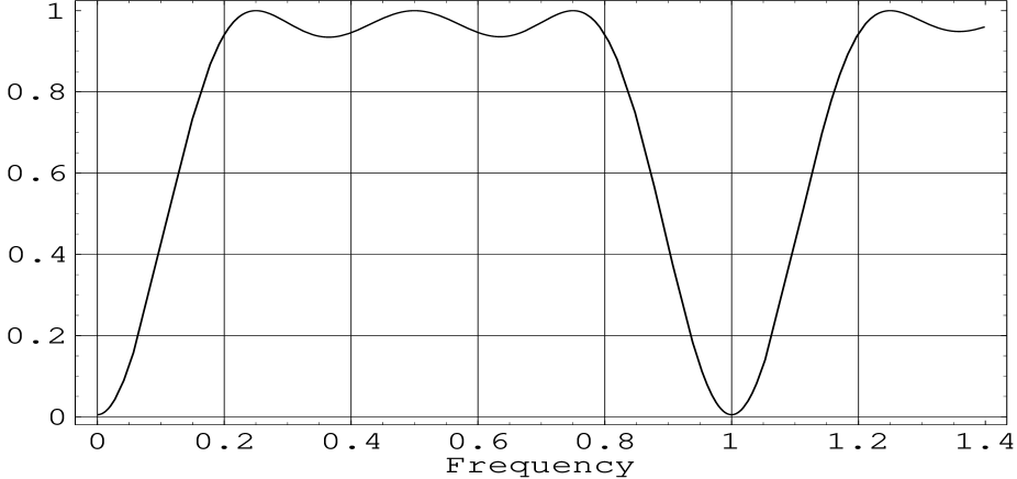
Figure 2: Plot of the Fourier transform of the filter function of timing residuals for the amount of orbital revolutions $N=4$. Frequency is measured in units of orbital frequency $n_{b}$. Amplitude of the transform has been normalized to unity.

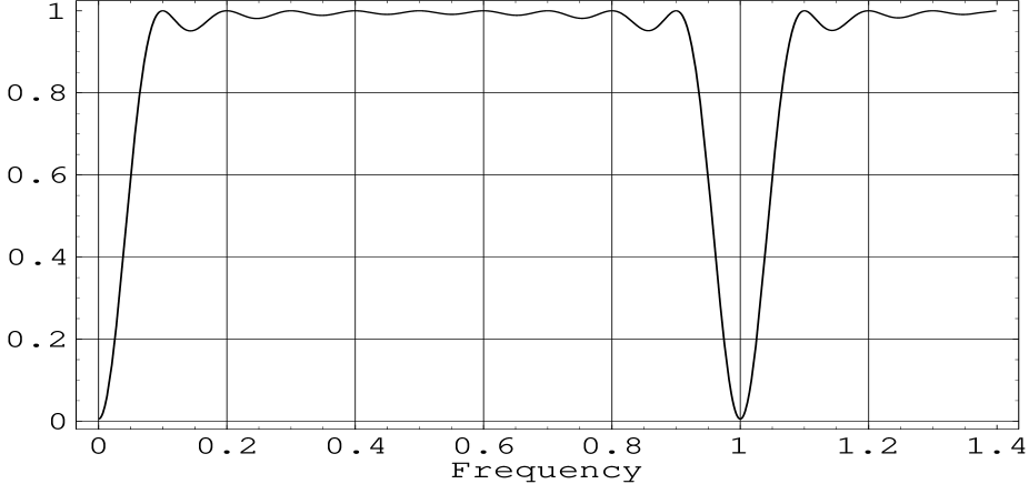
Figure 3: Plot of the Fourier transform of the filter function of timing residuals for the amount of orbital revolutions $N=10$. Frequency is measured in units of orbital frequency $n_{b}$. Amplitude of the transform has been normalized to unity.

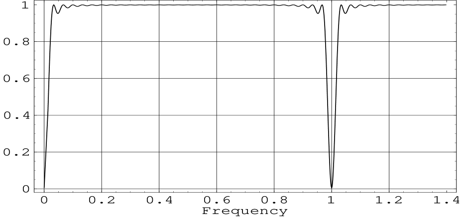
Figure 4: Plot of the Fourier transform of the filter function of timing residuals for the amount of orbital revolutions $N=30$. Frequency is measured in units of orbital frequency $n_{b}$. Amplitude of the transform has been normalized to unity.

References

- [1] Backer D.C., Kulkarni S.R., Heiles C., Davis M.M., Goss W.M., 1982, Nature, 300, 615
- [2] Bard Y., 1974, Nonlinear Parameter Estimation (Academic Press: New York)
- [3] Bell J.F., Bailes M., 1996, 456, L33
- [4] Bertotti B., Carr B.J., Rees M.J., 1983, MNRAS, 203, 945
- [5] Blandford R., Narayan R., Romani R., 1984, J. Astrophys. Astron., 5, 369
- [6] Camilo F., Foster R.S., Wolszczan A., 1994, ApJ, 437, L39
- [7] Cordes J.M., 1978, ApJ, 222, 1006
- [8] Cordes J.M., 1980, ApJ, 237, 216
- [9] Cordes J.M., Greenstein, G., 1981, ApJ, 245, 1060
- [10] Damour T., 1983a, Phys. Rev. Lett., 51, 1019
- [11] Damour T., Taylor J.H., 1991, ApJ, 366, 501
- [12] Damour T., Taylor J.H., 1992, Phys. Rev. D., 45, 1840
- [13] Deeter J.E., Boynton P.E., 1982, ApJ, 261, 337
- [14] Deeter J.E., 1984, ApJ, 281, 482
- [15] Deeter, J. E., Boynton P.E., Lamb, F. K., Zylstra, G., 1989, ApJ, 336, 376
- [16] Doroshenko O.V., Kopeikin S.M., 1990, Sov. Astron., 34, 496
- [17] Doroshenko O.V., Kopeikin S. M., 1995, MNRAS, 274, 1029
- [18] Gel’fand I.M., Shilov G.E., 1964, Generilized Functions: Properties and Operations (Academic Press, New York)
- [19] Grishchuk L.P., Kopeikin S.M., 1983, Sov. Astron. Lett., 9, 230
- [20] Groth E.J., 1975, ApJ Suppl., 29, 453
- [21] Ilyasov Yu.P., Kopeikin S.M., Rodin A.E., 1998, Astronomy Letters, 24, 228
- [22] Kaspi V.M., Taylor J.H., Ryba M.F., 1994, ApJ, 428, 713
- [23] Kopeikin S.M., 1988, Cel. Mech., 44, 87
- [24] Kopeikin S.M., 1994, ApJ, 434, L67
- [25] Kopeikin S.M., 1996, ApJ, 467, L93
- [26] Kopeikin S.M., 1997a, Phys. Rev. D, 56, 4455
- [27] Kopeikin S.M., 1997b, MNRAS, 288, 129
- [28] Kopeikin S.M., 1999, MNRAS, accepted for publication
- [29] Kopeikin S.M., Wex N., 1999, work in preparation
- [30] Korn G. A., Korn T. A., 1968, Mathematical Handbook for scientists and engineers (McGraw-Hill Book Comp., New York)
- [31] Mashhoon B., 1982, MNRAS, 199, 659
- [32] Mashhoon B., 1985, MNRAS, 217, 265
- [33] Mashhoon B., Seitz M., 1991, MNRAS, 249, 84
- [34] Matsakis D. N., Taylor J. H., Eubanks T. M., 1997 A&A, 326, 924
- [35] McHugh M.P., Zalamansky G., Vernotte F., Lantz E., 1996, Phys. Rev. D, 54, 5993
- [36] Newcomb S., 1898, Astron. Papers Am. Ephemeris Nautical Almanac, 6, 7
- [37] Peters P. C., Mathews J., 1963, Phys. Rev., 131, 435
- [38] Peters P. C., 1964, Phys. Rev., 136, 1224
- [39] Rawley L.A., Taylor J.H., Davis M.M., Allan D.W., 1987, Science, 238, 761
- [40] Rickett B. J., 1990, Ann. Rev. Astron. Astrophys., 28, 561
- [41] Rickett B. J., 1996, Interstellar Scaterring: Observations and Interpretations, In: Pulsars, Problems and Progress, eds. S. Johnston, M.A. Walker, M. Bailes, ASP Conf. Ser. 105, 439
- [42] Shabanova T.V., Il’in V.G., Ilyasov Yu.P., Ivanova Yu.D., Kuz’min A.D., Palii G.N., Shitov Yu.P., 1979,
- [43] Taylor J.H., 1991, Proc. IEEE, 79, 1054
- [44] Taylor J.H., Weisberg J.M., 1982, ApJ, 253, 908
- [45] Taylor J.H., Weisberg J.M., 1989, ApJ, 345, 434
- [46] Thorsett S.E., Dewey R.J., 1996, Phys. Rev. D, 53, 3468