1401998

Bose-Einstein Condensation of Atomic Hydrogen

1 INTRODUCTION

Bose-Einstein condensation in atomic hydrogen was observed for the first time just a few weeks before this session of the Enrico Fermi School, and so these lectures constitute a somewhat breathless first report. However, the search for Bose-Einstein condensation (BEC) in hydrogen began many years ago, and it has a long and colorful history. Out of that history emerged an extensive body of knowledge on the behavior of hydrogen at low temperatures that provided the foundation for achieving BEC in hydrogen. Much of it has been described in reviews [1, 2, 3, 4]. Consequently, we will dwell on only those features of that research that provide essential background, and concentrate on the most recent developments in which BEC in hydrogen advanced from a long period of being tantalizingly close, to being real.

2 ORIGINS OF THE SEARCH FOR BEC IN AN ATOMIC GAS

In April, 1976, W. C. Stwalley and L. H. Nosanow published a letter summarizing studies on the equation of state of spin-polarized hydrogen, $H\!\!\downarrow$ [5]. Because there are no bound states of molecular hydrogen in the triplet state, $H\!\!\downarrow$ behaves like a simple monatomic gas, but a gas with a remarkable property. Because of the weak $H\!\!\downarrow$ - $H\!\!\downarrow$ potential and the atom’s low mass, $H\!\!\downarrow$ remains a gas at temperatures down to $T=0$. Consequently, it might be possible to cool $H\!\!\downarrow$ to the quantum regime and achieve BEC. That paper essentially launched the search for BEC in an atomic gas. It triggered a flurry of experiments and enough activity for an entire session of the December, 1978, APS meeting to be devoted to the stabilization of hydrogen [6].

The critical density for the BEC transition in a non-interacting gas is $n_{\rm c}=2.612\Lambda_{\rm T}^{-3}$, where $\Lambda_{\rm T}=\sqrt{2\pi\hbar^{2}/k_{\rm B}Tm}$ is the thermal de Broglie wavelength. Because $n_{\rm c}$ depends on the product of temperature and mass, for a given density hydrogen condenses at a higher temperature than any other atom. Hydrogen offered two other attractions as a candidate for BEC. The hydrogen atom is generally appealing for basic studies because its structure and interactions can be calculated from first principles. Furthermore, $H\!\!\downarrow$ constitutes a nearly ideal Bose gas: it has an anomalously small $s$-wave scattering length and its interactions are weak.

In the years since the search for BEC in atoms started, there was a revolution in techniques for cooling and manipulating atoms using laser-based methods that culminated in the achievement of BEC in alkali metal atoms [7, 8, 9]. In light of these advances, hydrogen’s special attractions must be viewed from a new perspective. Spin-polarized hydrogen’s unique property of remaining a gas at $T=0$ is evidently not essential for BEC. Although all species except helium should be solid at sub-kelvin temperatures, laser-cooled atoms do not even liquefy because they never hit surfaces. In the absence of surface collisions, a gas to liquid transition requires three-body collisions to initiate nucleation. At the densities used to achieve BEC in alkali metal atom systems, however, the three-body recombination rate is so low that it can be neglected at all but the highest densities. Hydrogen’s relatively high condensation temperature is also not a crucial advantage. Laser cooling methods make it is possible to cool alkali metal gases to the microkelvin regime, far colder than possible by conventional cryogenic means. Once the atoms have achieved the laser-cooling temperature limit, they can be efficiently cooled into the nanokelvin regime by evaporative cooling. Finally, hydrogen’s close to ideal behavior must now be regarded as a serious experimental disadvantage. This is because all routes to BEC used so far involve evaporative cooling. Evaporation requires collisions for maintaining thermal equilibrium as the system cools. Because of hydrogen’s small scattering length, its collision cross section is tiny and evaporation is much slower than in other systems.

Nevertheless, now that hydrogen can be Bose-Einstein condensed, its simplicity continues to give the atom unique interest. The techniques, condensate size, and the general conditions for condensation are different from those of other realizations and one can expect that this new condensate will open complementary lines of research.

Spin polarized hydrogen is created by the magnetic state selection of hydrogen at cryogenic temperatures. In high magnetic fields the electron and proton spin quantum numbers are $m_{e}=-\frac{1}{2},~{}m_{p}=\pm\frac{1}{2}$ for $H\!\!\downarrow$  and $m_{e}=+\frac{1}{2},~{}m_{p}=\pm\frac{1}{2}$ for $H\!\!\uparrow$. The governing parameter in magnetic state selection is the interaction energy in a strong magnetic field, $B$. In temperature units, this is $T_{o}=\mu_{\rm B}B/k_{\rm B}=0.67(B/{\rm tesla})$ K. Here $\mu_{\rm B}$ is the Bohr magneton, and $k_{\rm B}$ is Boltzmann’s constant. For a field of $10$ T, which is readily achieved in a superconducting solenoid, $T_{o}=6.7$ K. At a temperature of $0.3$ K the ratio of densities $n$($H\!\!\uparrow$) / n($H\!\!\downarrow$) $\sim\exp(-2T_{o}/T)$, which is about $10^{-20}$. The spin polarization is essentially 100%.

Another crucial experimental parameter in creating $H\!\!\downarrow$ is the binding energy for adsorption on a liquid helium surface, $E_{\rm b}$. Hydrogen must make collisions with a cold surface in order to thermalize at cryogenic temperatures, but if the atoms become adsorbed the gas will rapidly recombine. In thermal equilibrium, the surface density $\sigma$ and volume density $n$ of $H\!\!\downarrow$ are related by $\sigma=\Lambda_{\rm T}n\exp{(-E_{\rm b}/k_{\rm B}T)}$. For hydrogen-helium, $E_{\rm b}=1$ K. Consequently, for temperatures below about 0.1 K the atoms move to the walls where they can recombine by two- and three-body processes. The initial searches for BEC were in the temperature regime $0.2\sim 0.7$ K. The critical density at a temperature of $0.5$ K is $n_{\rm c}=6.8\times 10^{19}~{}{\rm cm}^{-3}$.

Spin-polarized hydrogen was first stabilized by I. F. Silvera and J. T. M. Walraven in 1980 [10], and magnetically confined by the M.I.T. group [11]. In these experiments the field of a superconducting solenoid provided both state-selection and axial confinement. Radial confinement was provided by a superfluid helium-coated surface.

The highest density achieved with $H\!\!\downarrow$ under controlled conditions was $4.5\times 10^{18}~{}{\rm cm}^{-3}$, at a temperature of $0.55$ K [3]. The density was limited by three-body recombination, a process that had been predicted by Kagan et al. [12]. Because the heat generation in three-body recombination increases as the cube of the density, at higher density the gas would essentially self-destruct. An alternative route to BEC was required.

3 HYDROGEN TRAPPING AND COOLING

The new route toward BEC led to temperatures in the microkelvin regime where $n_{\rm c}$ is so low that three-body recombination is unimportant. At temperatures much below $0.1$ K, however, surface adsorption and recombination become prohibitive. To avoid surfaces, Hess suggested strategies for confining $H\!\!\uparrow$ atoms (in the “low field seeking” states) in a magnetic trap, and cooling the gas by evaporation [13].

Trapping and cooling requires an irreversible process for losing energy. In laser-cooling and trapping experiments, this process is spontaneous emission. Unfortunately, laser methods are not well suited to hydrogen. Aside from the lack of convenient light sources, the laser cooling temperature limit for hydrogen is relatively high. The limit is determined by the recoil energy for single photon emission, and in hydrogen it is more than a millikelvin. The method proposed by Hess employed elastic scattering for both trapping and cooling.

The magnetic trap proposed by Hess consists of a long quadrupole field to confine the atoms radially with axial solenoids at each end to provide axial confinement—an elongated variant of the “Ioffe-Pritchard” configuration [14]. The Ioffe-Pritchard potential is

$$V({\bf r})=\sqrt{(\alpha\rho)^{2}+(\beta z^{2}+\theta)^{2}}-\theta,$$ (1)

with radial potential gradient $\alpha$, axial curvature $2\beta$, and bias energy $\theta$. At low energies the potential is quasi-harmonic with radial and axial oscillation frequencies ω_ρ&= αm (βz2+θ)
ω_z = 2βm The trapping fields are produced inside a cell that confines the gas cloud while atoms are loaded into the trap. The walls of the helium-coated cell are held at a temperature of about 275 mK. The cell is filled with a puff of hydrogen and helium from a low temperature discharge and the walls of the cell are then cooled, making them “sticky.” Atoms with high energy leave the trap and stick to the walls. Thermal contact between the walls and the trapped gas is broken because these atoms are unable to return. The trapped gas cools by evaporation and reaches an equilibrium temperature of about 1/12th the trap depth.

To further cool the gas, Hess proposed a process of forced evaporation. The height of the potential barrier is slowly decreased, allowing energetic atoms to escape and thus reducing the average energy of the system. As the system’s reduced energy is redistributed by collisions, the temperature falls. Unlike ordinary evaporation which has a temperature limit determined by the vapor pressure of the material, forced evaporation can be continued to almost arbitrarily low temperatures. The process is surprisingly efficient because the escaping atoms carry away a great deal of energy, $(5\sim 10)k_{\rm B}T$ per atom.

Spin-polarized hydrogen was confined by a pure magnetic trap in 1987 by the M.I.T. group [15] and also in Amsterdam [16]. Shortly thereafter, in the first demonstration of forced evaporative cooling the M.I.T. group achieved a temperature of 3 mK [17].

In all of these experiments, the atoms were studied by monitoring the hydrogen flux as the atoms were dumped from the trap. With this technique [17, 18], the field of one of the axial confining coils is reduced, allowing the atoms to escape from the trap. Once out of the trap, the hydrogen rapidly adsorbs on the walls of the cell and recombines. This heat of molecular recombination—4.6 eV per event—is measured by a small bolometer within the cell but outside the trap. If the confinement field is reduced rapidly compared to the thermalization time, then the atom flux as a function of barrier height reveals the energy distribution of the gas. From this the temperature can be inferred. A typical energy distribution is shown in fig. 1.

Figure 1: Energy distribution of trapped $H\!\!\uparrow$ after evaporative cooling: plot of the atom flux as the trap barrier is rapidly lowered. The atom flux is measured by detecting the molecular recombination heat on a sensitive bolometer. Calculated distributions for three temperatures are shown.

Integrating the signal gives a measure of the total number $N$ of atoms trapped.

The density can also be determined by observing the decay of the trapped gas. The primary decay mechanism in $H\!\!\uparrow$ is dipolar relaxation, a process in which the spin angular momentum of a pair of atoms is transferred to their orbital angular momentum, while one or both of the atoms makes a transition to an untrapped state and escapes. Because dipolar relaxation is a two-body process, the density decays according to $\dot{n}=-gn^{2}$, where the dipolar decay constant $g$ has been calculated [19, 20] and also measured [15, 16]. The calculated value is $g=1.2\times 10^{-15}~{}{\rm cm}^{3}\rm s^{-1}$ [21]. The total sample decays according to $\dot{N}=-\kappa gN$ where

$$\kappa=\frac{\int\exp\left[-2V({\bf r})/k_{\rm B}T\right]dV}{\int\exp\left[-V({\bf r})/k_{\rm B}T\right]dV}.$$ (2)

For dipolar decay the number of trapped atoms decays according to

$$N(0)/N(t)=1+\kappa gn_{o}t.$$ (3)

Hence, the initial peak density $n_{o}$ can be extracted from a plot of $N(0)/N(t)$. An example of such a plot is shown in fig. 2.

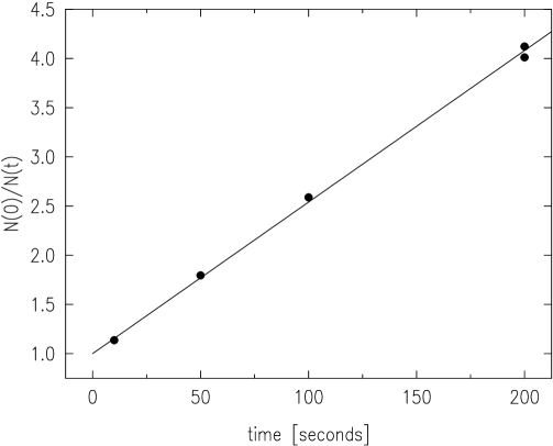
Figure 2: Determination of the sample density by observing decay due to dipolar relaxation. Five samples were indentically prepared and then held for varying times (horizontal axis) before being dumped from the trap. The integrated recombination signal from the dump gives the number of atoms in the trap, and is plotted on the vertical axis. The straight line fit indicates a density of $6.0\times 10^{13}~{}{\rm cm}^{-3}$. From [50]

Typically $\kappa\sim 1/5$ and the characteristic decay time at a density of $10^{14}~{}{\rm cm}^{-3}$ is 40 s.

Dipolar relaxation takes place predominantly where the density is high. This is at the minimum of the trap where the mean energy is low. Just as evaporation cools by removing the most energetic atoms, dipolar relaxation heats by removing the least energetic atoms. Consequently, the trapped gas comes to a thermal equilibrium in which cooling due to evaporation is balanced by heating due to dipolar relaxation.

These attempts to reach BEC in $H\!\!\uparrow$ stopped short of the quantum degenerate regime by about a factor of six in phase space density [22]. Several complications arose. The diagnostic technique of dumping the atoms out of the trap began to give ambiguous results because the energy distributions of the samples would change significantly during the dumping process. The sensitivity of the detection process was not sufficient. The efficiency of the evaporative cooling process degraded significantly, precluding further cooling. Finally, even if the quantum degnerate regime could be reached, a condensate would degenerate during the sample dumping process, and would have been unobservable. These complications required a new diagnostic technique and a more efficient evaporation process.

4 OPTICAL DETECTION OF TRAPPED HYDROGEN

Trapped hydrogen can be detected in situ by photoabsorption using one- and two-photon transitions. The Amsterdam group has used both methods. Using a Lyman-$\alpha$ light source they observed absorption of the principal transition [23]. However, the absorption spectrum has a large natural linewidth and displays structure due to the inhomogeneous magnetic field, limiting its use for analyzing momentum. They also observed the $1S$-$3S$ and $1S$-$3D$ transitions using resonantly enhanced two-photon excitation exploiting a virtual state near $2P$ [24]. The $1S$-$3S$ transition is insensitive to magnetic fields and is potentially well suited for analyzing momemtum at temperatures down to 1 $\mu$K. The $1S$-$3D$ transition has a matrix element that is ten times larger, but a natural linewidth that is ten times broader.

We have employed two-photon Doppler-free spectroscopy of the $1S$-$2S$ transition, using two-photons from a single laser tuned to 243 nm, twice the Lyman-$\alpha$ wavelength. The spectrum is essentially unperturbed by the magnetic field. This method provides excellent momentum resolution but suffers from the low excitation rate of a forbidden transition. In two-photon spectroscopy using a single light source normally only the narrow Doppler-free spectrum is observed, excited by counter-propagating laser beams that eliminate the first order Doppler effect. However, at very low temperatures in our experiment the broad Doppler-sensitive spectrum is also visible, excited by absorbing two photons from the same laser beam. Because the momentum distribution in a condensate is much narrower than in a normal gas at the same temperature, the Doppler-sensitive spectrum is well suited to probing the condensate. In addition to its application to observing BEC, Doppler-free spectroscopy of cold trapped hydrogen has a potential application to the precision spectroscopy of hydrogen, in which the $1S$-$2S$ transition plays a central role [25]. Under suitable conditions, time-of-flight broadening disappears and a spectral resolution close to the natural linewidth of 1.3 Hz should be possible [26].

In our method [27], the atoms are excited by a pulse of 243 nm radiation. For observing BEC the pulse length is typically 0.4 ms, but for spectroscopic studies pulses as long as 5 ms have been used. (In the absence of an electric field we have observed that the $2S$ atoms live for close to the natural lifetime, 122 ms [27].) Because of the low excitation rate, it is not feasible to observe photoabsorption. Instead, the excited atoms are detected by switching on an electric field which Stark-quenches the $2S$ state, mixing it with the $2P$ state which promptly decays. The emitted Lyman-$\alpha$ photon is detected. A diagram of the apparatus is shown in fig. 3.

Figure 3: Schematic diagram of the apparatus. The superconducting magnetic coils create trapping potential that confines atoms near the focus of the 243 nm laser beam. The beam is focused to a 50 $\mu$m waist radius and retroreflected to produce the standing wave required for Doppler-free two-photon absorption. After excitation, fluorescence is induced by an applied electric field. A small fraction of the 122 nm fluorescence photons are counted on a microchannel plate detector. The bolometer is used for diagnostic purposes. Not shown is the trapping cell which surrounds the sample and is thermally anchored to a dilution refrigerator. The actual trap is longer and narrower than indicated in the diagram.

The energy equation for two-photon excitation of an atom from state $i$ to $f$, with initial momentum ${\bf p}_{i}$ and final momentum ${\bf p}_{f}={\bf p}_{i}+\hbar({\bf k}_{1}+{\bf k}_{2})$, where ${\bf k}_{1}$ and ${\bf k}_{2}$ are the wave vectors of the laser beams, is

$$2h\nu=\sqrt{p_{f}^{2}c^{2}+(mc^{2}+2h\nu_{o})^{2}}-\sqrt{p_{i}^{2}c^{2}+(mc^{2})^{2}}.$$ (4)

where the rest mass of the atom in the initial state is $m$ and $\nu_{o}$ is the unperturbed transition frequency. Expanding, we obtain

$$\nu=\nu_{o}+\underbrace{\frac{({\bf k}_{1}+{\bf k}_{2})\cdot{\bf p}_{i}}{4\pi m}\left(1-\epsilon\right)}_{\textstyle\Delta\nu_{D1}}+\underbrace{\frac{\hbar({\bf k}_{1}+{\bf k}_{2})^{2}}{8\pi m}\left(1-\epsilon\right)}_{\textstyle\Delta\nu_{R}}-\underbrace{\frac{\nu_{o}p_{i}^{2}}{2(mc)^{2}}}_{\textstyle\Delta\nu_{D2}}+O{\left(\frac{h\nu}{mc^{2}}\right)^{3}}.$$ (5)

Here $\Delta\nu_{D1}$ and $\Delta\nu_{D2}$ are the first and second order Doppler shifts, respectively, $\Delta\nu_{R}$ is the recoil shift, and $\epsilon=2h\nu_{o}/mc^{2}=1.1\times 10^{-8}$ is a relativistic correction which accounts for the mass change of the atom upon absorbing energy $2h\nu_{o}$. For hydrogen in the submillikelvin regime, $\Delta\nu_{D2}\ll 1$ Hz, and can be neglected. In the Doppler-sensitive configuration, ${\bf k}_{1}={\bf k}_{2}$ and $\Delta\nu_{R}=6.7$ MHz. (All frequencies are referenced to the 243 nm laser source). At a temperature of $50~{}\mu$K, $\Delta\nu_{D1}\sim 2.6$ MHz. In the Doppler-free configuration, ${\bf k}_{1}=-{\bf k}_{2}$, and there is no recoil or first order Doppler broadening. Doppler-free excitation is achieved by retro-reflecting the laser beam. Nevertheless, in this configuration the Doppler-sensitive line is also excited, with the atom absorbing two photons from a single laser beam.

Far from quantum degeneracy, the lineshape for Doppler-sensitive excitation is the familiar Gaussian curve characteristic of a Maxwell-Boltzmann distribution. The shape for Doppler-free excitation, however, is quite different—a cusp-shaped double exponential [28]: $I(\nu-\nu_{o})\sim\exp(-\mid\nu-\nu_{o}\mid/\delta_{o})$. The linewidth parameter $\delta_{o}$ is determined by the time of flight of an atom across the laser beam: $\delta_{o}=u/2\pi d_{o}$ where $u=\sqrt{2k_{\rm B}T/m}$ is the most probable velocity and $d_{o}$ is the waist diameter of the laser beam. This expression is valid for an untrapped gas far from quantum degeneracy. It neglects collisions and other broadening mechanisms, and the natural linewidth of 1.3 Hz. An example of this Doppler-free lineshape is shown in fig. 4.

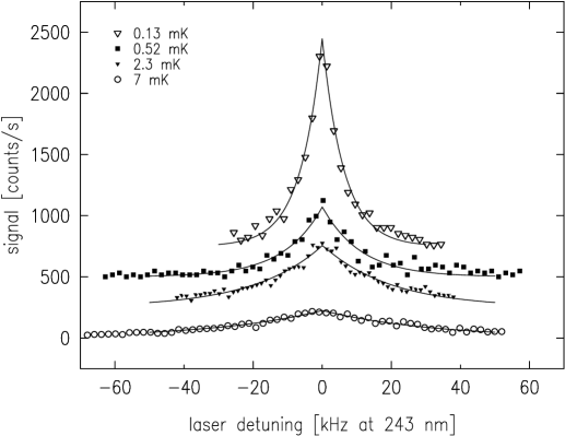
Figure 4: Spectra of low density samples at a series of temperatures. The linewidth is given by the finite interaction time as an atom traverses the Gaussian laser beam. The exponential lineshape arises from an average over a Maxwell-Boltzmann distribution of velocities. As the sample cools, the characteristic velocity decreases and the line narrows $\sim\sqrt{T}$. The laser power was about 7 mW, and densities were in the range $10^{12}\sim 10^{13}{\rm cm}^{-3}.$

A panoramic spectrum showing the Doppler-free and the recoil-shifted Doppler-sensitive lines is shown in fig. 5.

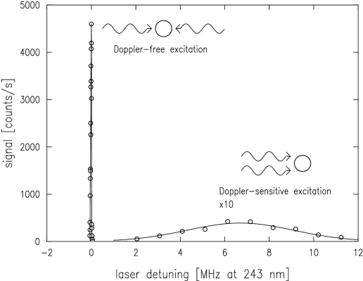
Figure 5: Composite $1S$-$2S$ two-photon spectrum of trapped hydrogen before condensation. The intense, narrow peak arises from absorption of counter-propagating photons by the normal gas, and exhibits no first-order Doppler broadening. The wide, low feature on the right is from absorption of co-propagating photons. The solid line is the recoil-shifted, Doppler-broadened, Gaussian lineshape of the normal gas corresponding to $T=40~{}\mu$K. Zero detuning is taken for unperturbed atoms excited Doppler-free. All frequencies are referenced to the $243$ nm excitation radiation.

If the atoms are confined in a radially harmonic trap, the Doppler-free spectrum consists of a central line at frequency $\nu_{o}$ plus a series of sidebands spaced by twice the trap frequency, lying under the exponential curve [29]. The intensity of the sidebands is governed by the ratio of the atom cloud diameter to laser beam diameter. If this ratio is less than 1, only the cental line is excited, an example of Dicke narrowing.

5 EVAPORATIVE COOLING

The physical principles and experimental considerations of evaporative cooling have been described in detail by Ketterle and van Druten [30]. We summarize here some of the principal points.

Evaporative cooling occurs when highly energetic atoms are permitted to escape from a trap at a rate that is kept sufficiently low for the remaining gas to maintain a quasi-thermal equilibrium. In this situation the energy distribution is thermal except that it is truncated at the depth of the trap, $V_{\rm trap}$. The crucial parameters governing evaporative cooling are:

The elastic collision rate. This determines the rate of thermalization. The low temperature collision cross section in a Bose gas is determined by the $s$-wave scattering length, $a$. The elastic collision cross section for identical particles is $\sigma_{\rm el}=8\pi a^{2},$ and the elastic collision rate is $\Gamma_{\rm el}=\sqrt{2}n\sigma_{\rm el}\bar{v}$, where $n$ is the density and $\bar{v}=\sqrt{8k_{\rm B}T/\pi m}$. Table 1 shows values of $a$ and $\sigma_{\rm el}$ for hydrogen and a number of alkali metal atoms.

species	$m$ (amu)	$a$ (nm)	$\sigma_{\rm el}$ (cm2)	$T_{c}$ ($\mu$K)	$n_{c}$ (cm-3)	$N_{c}$
H [31]	1	0.0648 [32]	$1.06\times 10^{-15}$	50	$1.8\times 10^{14}$	$10^{9}$
Li [33]	7	-1.45 [34]	$5.2\times 10^{-13}$	0.30	$1.5\times 10^{12}$	$10^{3}$
Na [35]	23	2.8 [36]	$1.90\times 10^{-12}$	2.0	$1.5\times 10^{14}$	$10^{7}$
Rb [37]	87	5.4 [38]	$7.3\times 10^{-12}$	0.67	$2.2\times 10^{14}$	$2\times 10^{6}$

Table 1: Comparison of the atomic species that have been Bose condensed. For each cited experiment, $a$ is the scattering length, $\sigma_{\rm el}$ is the elastic scattering cross section, $T_{c}$ is the temperature of the onset of BEC, $n_{c}$ is the density of the thermal cloud at the onset, and $N_{c}$ is the maximum number of condensate atoms.

Hydrogen’s anomalously small scattering length is conspicuous. In consequence, its elastic scattering cross section is smaller than that of the alkali metal atoms by a factor of a thousand or more, and evaporative cooling proceeds at a correspondingly low rate.

The cooling path. The ratio of trap depth to thermal energy, $\eta\equiv V_{\rm trap}/k_{\rm B}T$ is an important parameter in determining the most efficient evaporation path. The rate at which atoms with enough energy to escape from the trap are generated is approximately proportional to $\eta\exp(-\eta)$. Each atom carries away energy $\sim\eta k_{\rm B}T$. If $\eta$ is large, each escaping atoms carries away a great deal of energy, enhancing the efficiency of cooling, but because the number of these atoms is small, their evaporation proceeds slowly. If $\eta$ is too small, the atoms can escape too rapidly for the system to thermalize, and the efficiency falls.

Trap geometry. In a square-well potential, the density of a trapped gas is independent of its energy, and the elastic collision rate $\Gamma_{\rm el}=\sqrt{2}n\bar{v}\sigma$ decreases as $\bar{v}\sim\sqrt{T}$: evaporation slows as the temperature falls. In a trap, however, as the cloud cools the atoms are compressed into the region of lowest potential, and the density of the gas increases as its temperature falls. As a result, in a harmonic trap the evaporation rate increases with falling temperature as $\Gamma_{\rm el}\sim T^{-1}$. In a quadrupole trap, $\Gamma_{\rm el}\sim T^{-5/2}$. Consequently, the functional form of the trap shape is a critical design factor. Because the evaporation rate in a trap increases as the temperature falls, one can achieve conditions of runaway evaporation in which evaporation, once started, can proceed faster and faster.

Loss processes. If there were no loss mechanisms in the trapped gas, the time for evaporation could be made as long as desired and the magnitude of $\Gamma_{\rm el}$ would be unimportant. However, loss processes are inevitable. In experiments with alkali metal atoms the principal loss is scattering of atoms out of the trap by collisions with the warm background gas in the cell. The loss rate is independent of the density of the trapped gas. (At very high density, however, loss due to 3-body recombination plays the limiting role.) In the cryogenic environment of atomic hydrogen experiments, the major loss process is dipolar decay at a rate proportional to density. Because both the dipolar decay rate and $\Gamma_{\rm el}$ vary linearly with density, the conditions for runaway evaporation are not achieved.

6 EVAPORATION TECHNIQUES

In the initial demonstration of evaporative cooling the atoms were permitted to escape over a saddle point in the magnetic field at one end of the long cylindrical trap. Evaporation is forced by lowering this axial confinement field while simultaneously holding the radial confinement fields fixed. Energetic atoms are able to escape out the end of the trap. With this method, called saddle point evaporation, it was possible to achieve conditions close to BEC in hydrogen, but the cooling power was not adequate to cross the barrier.

The inefficiency of the evaporation process has been explained by Surkov et al. [39]. In saddle point evaporation atoms escape only along the z-axis. For an atom to escape, it must have a sufficient energy in the axial degree of freedom, $E_{z}\geq V_{\rm trap}$, where $V_{\rm trap}$ is the trap depth as set by the saddle point potential. Because only the $z$-motion is involved, the evaporation is inherently one-dimensional. If the axial and radial motion mix rapidly, then all atoms with total energy $E\geq V_{\rm trap}$ can promptly escape. At high energy this mixing takes place in our trap because of the coupling of radial and transverse co-ordinates.

As the energy decreases and the trap becomes more harmonic, the mixing time lengthens. When it becomes comparable to the collision time, the evaporation rate falls. This is because the collision of an energetic atom generally transfers it to lower energy: the atom is knocked back into a trapped energy regime. Mixing is governed by the adiabaticity parameter, $\Phi=\dot{\omega}_{\rho}/\omega_{\rho}^{2}$, which quantifies the fractional change in the radial oscillation frequency per oscillation period as the atom moves along the trap axis (see eq. 1). For $\Phi\ll 1$, the probability of transfering the energy from radial to longitudinal during one radial oscillation is $\sim\Phi$. Using $\dot{\omega}_{\rho}=(\drm\omega_{\rho}/\drm z)(\drm z/\drm t)$ we obtain

$$\Phi=v_{z}\>\frac{\beta z\sqrt{m}}{\alpha\sqrt{\beta z^{2}+\theta}}.$$ (6)

For our trap at the threshold for BEC, $\Phi\sim 10^{-3}.$ However, the probability for scattering during a radial period, $2\pi\Gamma_{\rm el}/\omega_{\rho}$, is about ten times higher. Hence, the evaporation is essentially one-dimensional. Surkov et al. have shown that in this situation the cooling rate decreases by a factor of about $4\eta$ compared to the rate at which evaporation would proceed in three dimensions [39]. For hydrogen, such a decrease in the already low evaporation rate proves fatal. The effects of one-dimensional evaporation have been studied by Pinske et al. [40].

The bottleneck of saddle point evaporation is avoided by the technique of radiative evaporation, “rf evaporation,” originally proposed by Pritchard [41], which permits evaporation in three dimensions. A radio-frequency oscillating magnetic field drives transitions between the trapped state and some other (untrapped) hyperfine sub-level, causing the atom to be ejected from the trap. In hydrogen the trapped hyperfine state is ($F=1,m=1$), and the rf transition is predominantly to the state (1,0). The resonance occurs for atoms in a region of the trap where the field magnitude $B_{0}$ satisfies the resonance condition $\hbar\omega_{rf}=\mu_{\rm B}B_{0}$. Here $\mu_{\rm B}B_{0}$ is the Zeeman splitting between the hyperfine sub-levels. The transition matrix element is $\hbar\Omega_{R}=\mu_{\rm B}B_{\perp}/\sqrt{2}$, where $B_{\perp}$ is the amplitude of the rf field perpendicular to $B_{0}$. The probability of an atom experiencing a hyperfine sub-level transition as it traverses the resonance region can be estimated using the Landau-Zener theory. The trapping field is assumed to vary linearly with gradient $B^{\prime}$ in the vicinity of the resonance, and the atom traverses the region at speed $v$. The probability of a two-level atom making a transition as it traverses the resonance region is $p=1-\exp(-\zeta)$ where $\zeta=2\pi\hbar\Omega_{R}^{2}/\mu_{\rm B}B^{\prime}v$ [42]. The hydrogen $F=1$ state is actually a three level system. Vitanov and Suominen have solved the multilevel Landau-Zener problem [43], and we apply their results to our situation. The probability $P_{m}$ that an atom originally in the state (1,1) emerges in the state $(1,m)$ is P_1 &= (1-p)^2
P_0 = 2(1-p)p
P_-1 = p^2 For large $\zeta$ the atom absorbs two rf photons and emerges in the (1,-1) state, which is ejected. In our experiment $\zeta$ is small, and there is only a small probability of leaving the trapped (1,1) state. Transitions are primarily to the (1,0) state. Atoms in this state simply fall out of the trap.

For small $\zeta$, the probability of being ejected during one radial oscillation is $\sim 4\zeta$. As in the previous discussion on radial and longitudinal mixing, scattering sets a lower limit of $\zeta\geq 10^{-3}$. This requires a Rabi frequency of $\Omega_{R}\geq 2\pi\times 1$ kHz or an rf field strength $B_{\perp}\geq 10^{-7}$ T. (In other atomic systems dipolar relaxation can impose a more stringent requirement on the transition rate [30].)

To implement rf evaporation in a cryogenic environment methods had to be developed to eliminate eddy current losses and rf shielding by the cell. This was accomplished using a plastic cell design in which heat transport is provided by a superfluid helium jacket around the cell. The rf field amplitude is typically $7\times 10^{-7}$ T, and fields can be applied with frequencies up to 46 MHz. RF evaporation is switched on at a trap depth of about 1.1 mK, where the sample temperature is typically 120 $\mu$K.

In addition to driving evaporation, the rf field is used to find the temperature of the sample. The temperature is measured by sweeping the rf resonance through the trap and measuring the atom ejection rate as a function of frequency [41].

The field at the bottom of the trap, the axial bias field $\theta/\mu_{\rm B}$, is a critical parameter because it determines the curvature of the potential minimum and provides the zero point for determining the trap depth. If the field is too large the trap is harmonic, the effective volume is large, and the density is small. If the bias field is too low, the condensate is strongly confined and suffers a high dipolar decay rate. The optimum bias field is approximately $k_{\rm B}T/\mu_{\rm B}$. In such a field the thermal cloud is tightly confined, but the condensate can spread out due to interactions. In our experiments the bias field energy is about $\theta\simeq(3/5)k_{\rm B}T$. The bias field is measured by applying the rf field at a low frequency and sweeping the frequency up until atoms start to leave the trap.

We have neglected the effect of gravity. For $H\!\!\uparrow$ at a temperature of $50~{}\mu$K the gavitational scale height $k_{\rm B}T/mg$ is 4 cm, which is comparable to the vertical size of the cloud. For higher mass atoms, which condense at lower temperatures, gravity can be important. In such a case the surface of constant $B_{0}$ is no longer an equipotential. Evaporation occurs primarily from the bottom of the cloud, and becomes one-dimensional [30].

7 COLD-COLLISION FREQUENCY SHIFT

At low temperature, in the limit $a\ll\Lambda_{\rm T}$, only $s$-wave collisions are important. These collisions give rise to a mean interaction energy, and they introduce frequency shifts into radiative transitions. Such effects can be analyzed by kinetic theory starting with the Boltzmann transport equation [44, 45], or described by mean field theory based on the pseudopotential [46]. Both approaches give the same result for a homogenous system: the mean field energy of an atom in a gas with density $n$ is

$$\tilde{U}n=\frac{4\pi\hbar^{2}a}{m}n\times g_{2}(0),$$ (7)

where the density normalized second order correlation function $g_{2}(\bf{x})$ is [47]

$$g_{2}({\bf x})=\frac{1}{nN}\sum_{i\neq j}\left\langle\Psi\mid\delta({\bf r_{i}}-{\bf r_{j}}-{\bf x})\mid\Psi\right\rangle.$$ (8)

Here $\Psi$ is the wave function for the system. (For a Bose gas far from degeneracy, $g_{2}(0)=2$.) Because the scattering lengths for $1S$-$1S$ and $1S$-$2S$ collisions are not identical, the energy to excite an atom to the $2S$ state from a gas of $1S$ atoms is shifted by an amount [48]

$$h\Delta\nu_{\rm col}=\frac{4\pi\hbar^{2}n}{m}(a_{1S-2S}-a_{1S-1S})g_{2}(0).$$ (9)

The frequency shift $\Delta\nu_{\rm col}$ is known as a cold collision frequency shift. For a non-degenerate gas the two-photon sum frequency is shifted by $\Delta\nu_{\rm col}=n\chi$, where $\chi=4\hbar(a_{1S-2S}-a_{1S-1S})/m$. Once $\chi$ is known, the density can be determined directly by measuring the frequency shift. In addition, a measurement of $\chi$ can be used to check the theoretical calculations of the scattering lengths. The $1S$-$1S$ scattering length is known accurately from theory: $a_{1S-1S}=0.0648$ nm [32], and $a_{1S-2S}$ has also been computed: $a_{1S-2S}=-2.3$ nm [49].

The cold-collision shift of the $1S$-$2S$ transition plays a key role in our experiments, allowing us to measure the density rapidly in situ. Furthermore, because the density in a Bose-Einstein condensate in $H\!\!\uparrow$ is much higher than the density of the normal gas, the cold-collision frequency shift provides an unmistakable signature of the condensate.

To measure the frequency shift parameter $\chi$, a series of line scans were taken at different densities as shown in fig. 6a.

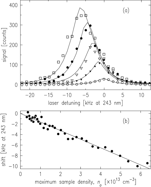
Figure 6: (a) Series of spectra of a single sample used for a measurement of $\chi$. The first scan is at the maximum density and exhibits the largest red shift. Subsequent scans, at lower densities, are smaller and less shifted. Five of the forty spectra are shown. (b) Shift of the spectrum as a function of sample density. The density is inferred from the integrated signal. For this particular sample $\chi=-3.30\pm 0.6\times 10^{-10}{\rm~{}Hz~{}cm}^{3}$. From [50].

The initial density was established by monitoring the two-body dipolar decay rate, as described above. During successive laser scans of a single trapped sample the density decayed because of collisions with helium gas generated by heating due to the laser. The area under each photoexcitation curve is proportional to the total number of atoms, making it possible to infer the density for each scan. The line center for each curve was corrected for the effects of density inhomogeneities due to the trapping potential. From a plot of frequency vs. density, like the one shown in fig. 6b, the value of $\chi$ can be determined. From a series of such measurements taken at different densities and temperatures, we obtained $\chi=-3.8\pm 0.8\times 10^{10}~{}n~{}{\rm Hz\,cm}^{3}$. The theory of cold-collision frequency shifts in an inhomogeneous system is not yet fully understood, but assuming eq. 9 is still valid, we deduce $a_{1S-2S}=-1.4\pm 0.3$ nm, in fair agreement with the prediction [50].

8 OBSERVATION OF THE CONDENSATE

Bose-Einstein condensation in hydrogen was achieved at a temperature of about $50~{}\mu$K with a density of $1.8\times 10^{14}~{}{\rm cm}^{-3}$ [31]. Its onset was revealed by unmistakable new features in the spectrum, shown in fig. 7.

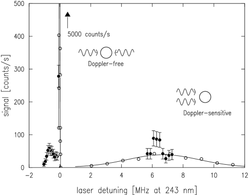
Figure 7: Composite $1S$-$2S$ two-photon spectrum of trapped hydrogen after condensation. $\circ$–spectrum of sample without a condensate; $\bullet$–spectrum emphasizing features due to a condensate. The high density in the condensate shifts a portion of the Doppler-free line to the red. The condensate’s narrow momentum distribution gives rise to a similar feature near the center of the Doppler-sensitive line. From [31].

In the Doppler-sensitive line there is a narrow peak, shifted somewhat to the red of the line center, and there is a similar line to the red of the Doppler-free line. (Note: the Doppler sensitive peak was not observed until after these lectures.) The shift of these lines reveals a density significantly higher than in the normal gas, as expected for the condensate.

Before BEC was observed in the spectrum there were strong indications that condensation was taking place from a study of the evolution of the density of the thermal cloud with decreasing temperature. The density of the non-condensed gas fraction was determined from the cold-collision frequency shift; the temperature was inferred from the trap depth, set by the frequency of the rf signal. A plot is shown in fig. 8.

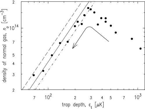
Figure 8: Density of non-condensed fraction of the gas as the trap depth is reduced along the cooling path. The density is measured by the optical resonance shift, and the trap depth is set by the rf frequency. The lines (dash, solid, dot-dash) indicate the BEC phase transition line, assuming a sample temperature of (1/5th, 1/6th, 1/7th) the trap depth. The scatter of the data reflects the reproducibility of the laser probe technique and is dominated by alignment of the laser beam to the sample. From [31].

In these observations the value of $\eta$ typically varied between 7 and 5 with decreasing temperature. The solid line in fig. 8 is the BEC boundary for $\eta=6$. Because the normal gas cannot exist to the left of the boundary, the density simply falls along the boundary. Once the system reaches the boundary, as the temperature is further reduced the normal atoms are forced into the condensate. Because the observations are at a laser frequency tuned so that only atoms from the normal gas are excited, the condensed atoms, which are at such a high density that they are frequency-shifted out of range, are not observed. Consequently, the density of the thermal cloud merely tracks the BEC line.

Because of the condensate’s high density, its dipolar decay rate is so high that, in isolation, it would disappear in about one second. However, because the condensate is continuously fed by the normal gas, its lifetime is several seconds. Its time evolution is shown in the series of spectral scans shown in fig. 9.

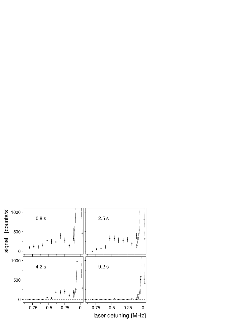
Figure 9: Time evolution of the condensate. Each spectrum is obtained in 0.67 s. As the condensate disappears the spectrum narrows, indicating a reduction in density, and gets weaker, indicating a reduction in condensate population. The last panel shows the background count rate. From [31].

As the density in the condensate decreases, the red shift decreases and the total signal becomes smaller, finally vanishing.

9 PROPERTIES OF THE CONDENSATE

The peak condensate density $n_{o,c}$ is found from the red cut-off of the spectrum. As shown in fig. 10,

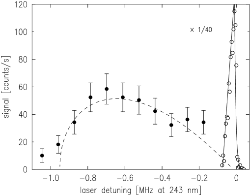
Figure 10: Doppler-free spectrum of the condensate (broad feature) and normal gas (narrow feature). The dashed line is proportional to the number of condensate atoms at a density proportional to the detuning, for an equilibrium density distribution with peak density $n_{o,c}=4.8\times 10^{15}~{}{\rm cm}^{-3}$ in a parabolic trap. From [31].

$n_{o,c}=4.8\pm 1.1\times 10^{15}~{}{\rm cm}^{-3}$. The peak mean field energy of an atom in the condensate, $\tilde{U}n_{o,c}/k_{\rm B}=4\pi\hbar^{2}an_{o,c}/k_{B}m=1.9~{}\mu$K, is much larger than the energy interval between the radial vibrational states of the trap, $\hbar\omega{\rho}/k_{\rm B}=190$ nK. Consequently, the shape of the condensate is determined by the mean field energy rather than the wave function of the trap’s ground state. The density profile, in the Thomas-Fermi approximation, is $n({\bf r})=n_{o,c}-V({\bf r})/\tilde{U}$.

With the Thomas-Fermi wavefunction, the total number of atoms in the condensate is found by integrating the density over the volume of the condensate. The result is

$$N_{c}=\frac{2^{9/2}\pi\;\tilde{U}^{3/2}\;n_{o,c}^{5/2}}{15\omega_{\rho}^{2}\;\omega_{z}\;m^{3/2}}=(1.1\pm 0.6)\times 10^{9}~{}{\rm atoms}.$$ (10)

The oscillation frequencies (eqs. 1) are $\omega_{\rho}=2\pi\times 3.90\pm 0.11$ kHz, and $\omega_{z}=2\pi\times 10.2$ Hz. The diameter of the condensate is $15~{}\mu$m and its length is $5$ mm. The huge aspect ratio, $\sim 400$, gives the condensate a thread-like shape.

The fraction of atoms in the condensate is small because the condensate is rapidly depleted by dipolar relaxation. The condensate size is limited by the low evaporative cooling rate in the normal gas, which supplies cold atoms to the condensate [51]. The fraction, $f={N_{c}}/(N_{n}+N_{c})$, can be found from the integrated area of the normal and condensate Doppler-free spectra, taking into account that although the entire condensate is in the laser beam, only a portion of the normal gas interacts with the laser. The condensate fraction can also be found by comparing the number of condensate atoms, determined from $n_{o,c}$ and the trap geometry, with the number of normal atoms found by integrating the Bose occupation function weighted by the trap density of states. (The temperature is measured from the Doppler-sensitive spectrum of the normal gas.) The trap shape cancels in the comparison. The methods are in good agreement at $f=6_{-3}^{+6}\%$. Both methods assume thermal equilibrium, which may not be justified.

In calculating the density and size of the condensate, we have taken $g_{2}(0)=1$ in computing the mean field energy (eq. 7), but $g_{2}(0)=2$ in calculating $n_{c,o}$ (eq. 9). Although this appears contradictory, it yields a condensate fraction that is consistent with the observed intensity ratio of the photoexcitation spectra and with the fraction predicted in ref. [51]. If we consistently take $g_{2}(0)=1$, then eq. 10 yields $N_{c}=6\times 10^{9}$ and $f=25\%$. If we consistently take $g_{2}(0)=2$, then $N_{c}=3\times 10^{9}$ and $f=14\%$. In a homogeneous condensate in thermal equilibrium one expects $g_{2}(0)=1$, however this may not apply under our experimental conditions. The problem clearly requires further study.

The Doppler-free lineshape of the normal gas displays puzzling behavior at the condensation transition. As seen in fig. 11,

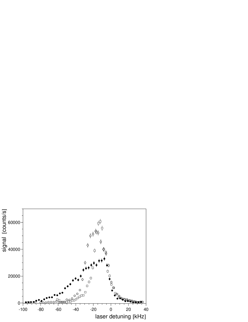
Figure 11: Doppler-free spectrum of normal fraction above and below the onset of BEC. The symmetric spectrum (above $T_{c}$, open symbols) suddenly becomes asymmetric (filled symbols) when the condensate forms. Temperatures for the three spectra are about $120~{}\mu$K (open squares), $53~{}\mu$K (open circles), $44~{}\mu$K (filled circles). From [31].

above the the transition temperature the line displays a roughly symmetric shape, as expected for the density distribution in the trap. When the condensate is present, the line develops a large asymmetry toward the red. The ratio of normal to condensate volumes is about $10^{3}$, so that this feature cannot be explained simply by penetration of the normal gas into the condensate.

10 PROSPECTS

As one expects whenever a novel system is created, the observation of BEC in hydrogen has led to some new questions. In particular, the nature of the photoexcitation spectrum from the condensate appears to be more subtle than previously appreciated. The cold-collision shift has proven to be an invaluable diagnostic tool, but beyond that it has led to an experimental value for an excited-state $s$-wave scattering length—the first such determination to our knowledge. One can conceive of methods for extending such measurements to other excited states.

Perhaps the most dramatic aspect of the hydrogen condensate is its size, more than thirty times larger than previous condensates, with prospects for large improvements. Thus, hydrogen should be a natural candidate for any application that requires an intense source of coherent atoms.

The techniques for achieving BEC in hydrogen evolved over a long time, and the apparatus reflects a great deal of history. Vast improvements would be possible if one were to start from scratch. In particular, the detection efficiency for Lyman-$\alpha$ photons is only about $2\times 10^{-5}$, the chief loss in signal being due to the low optical collection solid angle, $1.6\times 10^{-2}$ sr. An apparatus designed for optical access would provide a much higher signal rate, permitting a more precise study of the condensate’s properties and its dynamical behavior.

The size of the condensate is currently limited by the initial density of hydrogen that can be loaded into the trap. Improvements should be possible. On a more speculative note, if it were possible to increase the thermalization rate of a hydrogen sample by introducing an impurity atom into the trapped hydrogen gas, a major increase in the condensate size might be achieved.

11 Acknowledgements

Many people played important roles in the MIT work on spin-polarized hydrogen over the years. We especially wish to acknowledge those who contributed directly to the trapping and spectroscopy experiments: Claudio L. Cesar, John M. Doyle, Harald F. Hess, Greg P. Kochanski, Naoto Masuhara, Adam D. Polcyn, Jon C. Sandberg, and Albert I. Yu.

This research is supported by the National Science Foundation and the Office of Naval Research. The Air Force Office of Scientific Research contributed in the early phases. L.W. acknowledges support by Deutsche Forschungsgemeinschaft. D.L. and S.C.M. are grateful for support from the National Defense Science and Engineering Graduate Fellowship Program.

References

- [1] \BYGreytak, T. J. \atqueKleppner, D. in \TITLENew Trends in Atomic Physics, Les Houches Session 38, 1982 edited by \BYGrynberg, G., \atqueStora, R. (North Holland, 1984).
- [2] \BYSilvera, I. F., \atqueWalraven, J. T. M. in Progress in Low Temperature Physics, edited by \BYBrewer, D. F. \atqueStora, R. (North Holland, Amsterdam, 1984), p. 139.
- [3] \BYHess, H. F., Bell, D. A., Kochanski, G. P., Kleppner, D., \atqueGreytak, T. J. \INPhys. Rev. Lett.5219841520; \BYBell, D. A., Hess, H. F., Kochanski, G. P., Buchman, S., Pollack, L., Xiao, Y. M., Kleppner, D., \atqueGreytak, T. J. \INPhys. Rev. B3419867670.
- [4] \BYGreytak, T. J. in \TITLEBose-Einstein Condensation, edited by \BYGriffin, A., Snoke, D. W., \atqueStringari, S (Cambridge University Press, 1995), p. 131.
- [5] \BYStwalley, W. C., \atqueNosanow, L. H. \INPhys. Rev. Lett.361976910.
- [6] Bull. Am. Phys. Soc. 23, 85 (1978).
- [7] \BYAnderson, M. H., Ensher, J. R., Matthews, M. R., Wieman, C. E., \atqueCornell, E. A. \INScience2691995198.
- [8] \BYDavis, K. B., Mewes, M.-O., Andrews, M. R., Van Druten, N. J., Durfee, D. S., Kurn, D. M., \atqueKetterle, W. \INPhys. Rev. Lett.7519951687.
- [9] \BYBradley, C. C., Sackett, C. A., Tollet, J. J. , \atqueHulet, R. G. \INPhys. Rev. Lett.7519951687; \BYBradley, C. C., Sackett, C. A., \atqueHulet, R. G. \INPhys. Rev. Lett.781997985.
- [10] \BYSilvera, I. F. \atqueWalraven, J. T. M. \INPhys. Rev. Lett.441980164.
- [11] \BYCline, R. W., Greytak, T. J., \atqueKleppner, D. \INPhys. Rev. Lett.4719811195.
- [12] \BYKagan, Yu., Vartanyantz, I. A., \atqueShlyapnikov, G. V. \INSov. Phys. JETP541980590.
- [13] \BYHess, H. F. \INPhys. Rev. B3419863476.
- [14] \BYPritchard, D. \INPhys. Rev. Lett.5119831336.
- [15] \BYHess, H. F., Kochanski, G. P., Doyle, J. M., Masuhara, N. , Kleppner, D., \atqueGreytak, T. J. \INPhys. Rev. Lett.591987672.
- [16] \BYvan Roijen, R., Berkhout, J. J., Jaakkola, S., \atqueWalraven, J. T. M. \INPhys. Rev. Lett.611988931.
- [17] \BYMasuhara, N., Doyle, J. M., Sandberg, J. C., Kleppner, D., Greytak, T. J., Hess, H. F., \atqueKochanski, G. P. \INPhys. Rev. Lett.611988935.
- [18] \BYDoyle, J. M., Sandberg, J. C., Masuhara, N., Yu, I. A., Kleppner, D. \atqueGreytak, T. J. \INJ. Opt. Soc. Am. B619892244.
- [19] \BYLagendijk, A., Silvera, I. F., \atqueVerhaar, B. J. \INPhys. Rev. B31986626.
- [20] \BYStoof, H. T. C., Koelman, J. M. V. A., \atqueVerhaar, B. J. \INPhys. Rev. B3819884688.
- [21] In evaluating from [19] and [20], we have taken using the low field and zero temperature values for the rate constants. When one atom changes hyperfine state () both atoms are lost from the trap because the hyperfine energy (71 mK) is much greater than the trap depth.
- [22] \BYDoyle, J. M., Sandberg, J. C., Yu, I. A., Cesar, C. L., Kleppner, D., \atqueGreytak, T. J. \INPhys. Rev. Lett.671991603.
- [23] \BYSetija, I. D., Werij, H. G. C., Luiten, O. J., Reynolds, M. W., Hijmans, T. W., \atqueWalraven, J. T. M. \INPhys. Rev. Lett.7019932257.
- [24] \BYPinkse, P. W. H., Mosk, A., Weidemüller, M., Reynolds, M. W., Hijmans, T. W., \atqueWalraven, J. T. M. \INPhys. Rev. Lett.7919972423
- [25] \BYUdem, T., Huber, A., Gross, B., Reichert, J., Prevedelli, M., Weitz, M., \atqueHänsch, T. W. \INPhys. Rev. Lett.7919972646.
- [26] \BYKleppner, D. The Hydrogen Atom, ed. \BYBassani, G. F., Inguscio, M., \atqueHänsch, T. W. Springer Verlag (Berlin), 1989, p68.
- [27] \BYCesar, C. L., Fried, D. G., Killian, T. C., Polcyn, A. D., Sandberg, J. C., Yu, I. A., Greytak, T. J., Kleppner, D., \atqueDoyle, J. M. \INPhys. Rev. Lett.771996255.
- [28] \BYBordé, C. \INC. R. Hebd. Séan. Acad. Sci. B2821976341; \BYBiraben, F., Bassini, M., \atqueCagnac, B. \INJ. Phys. (Paris)401979445.
- [29] \BYCesar, C. L. Ph.D. thesis, M.I.T., 1997 (unpublished); \BYCesar, C. L. \atqueKleppner, D. to be published.
- [30] \BYKetterle, W. \atqueVan Druten, N. J. in Advances in Atomic, Molecular, and Optical Physics, edited by \BYBederson, B. \atqueWalther, H. (Academic Press, San Diego, 1996), No. 37, p. 181.
- [31] \BYFried, D. G., Killian, T. C., Willmann, L., Landhuis, D., Moss, S. C., Kleppner, D., \atqueGreytak, T. J. \INPhys. Rev. Lett.8119983811.
- [32] \BYJamieson, M. J., Dalgarno, A., \atqueKimura, M. \INPhys. Rev. A5119952626.
- [33] \BYBradley, C. C., Sackett, C. A., \atqueR. G. Hulet \INPhys. Rev. Lett.781997985.
- [34] \BYAbraham, E. R. I., McAlexander, W. I., Sackett, C. A., \atqueHulet, R. G. \INPhys. Rev. Lett.7419951315.
- [35] \BYStamper-Kurn, D. M., Andrews, M. R., Chikkatur, A. P., Inouye, S., Meisner, H.-J., Stenger, J., \atqueKetterle, W. \INPhys. Rev. Lett.8019982027.
- [36] \BYTiesinga, E., Williams, C. J., Julienne, P S., Jones, K M., Lett, P D., \atquePhillips, W D. \INJ. Res. Natl. Inst. Stand. Technol.1011996505.
- [37] \BYE. A. Burt, E. A., Ghrist, R. W., Myatt, C. J., Holland, M. J., Cornell, E. A., \atqueWieman, C. E. \INPhys. Rev. Lett.791997337.
- [38] \BYVogels, J. M., Tsai, C. C., Freeland, R. S., Kokkelmans, S. J. J. M. F., Verhaar, B. J., \atqueHeinzen, D. J. \INPhys. Rev. A561997R1067.
- [39] \BYSurkov, E. L., Walraven, J. T. M., \atqueShlyapnikov, G. V. \INPhys. Rev. A4919944778; \SAME5319963403.
- [40] \BYPinske, P. W. H., Mosk, A., Weidemüller, M., Reynolds, M. W., \atqueHijmans, T. W. \INPhys. Rev. A.5719984747.
- [41] \BYPritchard, D. E., Helmerson, K., \atqueMartin, A. G. in Atomic Physics 11, edited by \BYHaroche, S., Gay, J. C., \atqueGrynberg, G. (World Scientific, Singapore, 1989) p. 179.
- [42] \BYRubbmark, J. R., Kash, M. M., Littman, M. G., \atqueKleppner, D. \INPhys. Rev. A2319813107.
- [43] \BYVitanov, N. V. \atqueSuominen, K.-A. \INPhys. Rev. A561997R4377.
- [44] \BYVerhaar, B. J., Koelman, J. M. V. A., Stoof, H. T. C., \atqueLuiten, O. J. \INPhys. Rev. A3519873825.
- [45] \BYTiesinga, E., Verhaar, B. J., Stoof, H. T. C., \atqueVan Bragt, D. \INPhys. Rev. A451992R2671.
- [46] \BYPathria, R. K. Statistical Mechanics (Pergamon Press, New York, 1972), p. 300.
- [47] \BYVan Hove, L. \INPhys. Rev.951954249.
- [48] A different expression was presented in the lecture, and this expression requires some justification. It is not obvious that the - scattering leads to the same expression for the mean field energy as - scattering. The reason has to do with the nature of excitation, in which not one particular atom is excited but every atom is given a small component of excitation. Details will be published elsewhere.
- [49] \BYJamieson, M. J., Dalgarno, A., \atqueDoyle, J. M. \INMol. Phys.871996817.
- [50] \BYKillian, T. C., Fried, D. G., Willmann, L., Landhuis, D., Moss, S. C., Greytak, T. J., \atqueKleppner, D. \INPhys. Rev. Lett.8119983807.
- [51] \BYHijmans, T. W., Kagan, Yu., Shlyapnikov, G. V., \atqueWalraven, J. T. M. \INPhys. Rev. B48199312886.