CERN–TH 98-351

ISN 98–21

ON THE STABILITY DOMAIN OF SYSTEMS

OF THREE ARBITRARY CHARGES^†

Ali Krikeb⁽¹⁾, André Martin^(2),(3),

Jean-Marc Richard⁽⁴⁾ and Tai Tsun Wu${}^{\,\star}$$\,{}^{(2),(5)}$

${}^{(1)}\,$ Institut de Physique Nucléaire de Lyon-CNRS-IN2P3
Université Claude Bernard, Villeurbanne, France ${}^{(2)}\,$ CERN, Theory Division, CH 1211 Genève 23
${}^{(3)}\,$LAPP, B.P. 110, F-74941 Annecy Le Vieux, France
${}^{(4)}\,$Institut des Sciences Nucléaires–CNRS–IN2P3
Université Joseph Fourier
53, avenue des Martyrs, F-38026 Grenoble, France
${}^{(5)}\,$Gordon McKay Laboratory
Harvard University, Cambridge, Massachusetts
Abstract

We present results on the stability of quantum systems consisting of a negative charge $-q_{1}$ with mass $m_{1}$ and two positive charges $q_{2}$ and $q_{3}$, with masses $m_{2}$ and $m_{3}$, respectively. We show that, for given masses $m_{i}$, each instability domain is convex in the plane of the variables $(q_{1}/q_{2},\,q_{1}/q_{3})$. A new proof is given of the instability of muonic ions $(\alpha,p,\mu^{-})$. We then study stability in some critical regimes where $q_{3}\ll q_{2}$: stability is sometimes restricted to large values of some mass ratios; the behaviour of the stability frontier is established to leading order in $q_{3}/q_{2}$. Finally we present some conjectures about the shape of the stability domain, both for given masses and varying charges, and for given charges and varying masses.

${}^{\dagger}\,$ Dedicated to the memory of Harry Lehmann
${}^{\star}\,$Work supported in part by the U.S. Department of Energy under Grant No. DE-FG02-84-ER40158.
CERN–TH 98-351

.

1 Introduction

In two previous papers [1, 2], hereafter referred to as I and II, respectively, we studied the stability of quantum systems consisting of point-like electric charges

$$Q_{i}=\pm[-q_{1},q_{2},q_{3}],\qquad q_{i}>0,$$ (1)

and masses $m_{i}$. The Hamiltonian is

$$H={\vec{\rm p}_{1}^{2}\over 2m_{1}}+{\vec{\rm p}_{2}^{2}\over 2m_{2}}+{\vec{\rm p}_{3}^{2}\over 2m_{3}}-{q_{12}\over r_{12}}-{q_{13}\over r_{13}}+{q_{23}\over r_{23}},$$ (2)

where $q_{ij}=q_{i}q_{j}$ and $r_{ij}=|\vec{\rm r}_{i}-\vec{\rm r}_{j}|$.

In I, we considered the case of unit charges $q_{i}=1$, with application to physical systems such as ${\rm H}{{}_{2}}^{+}({\rm e}^{-}{\rm p}{\rm p})$, ${\rm H}^{-}({\rm p}{\rm e}^{-}{\rm e}^{-})$ and ${\rm Ps}^{-}({\rm e}^{+}{\rm e}^{-}{\rm e}^{-})$, which are stable, or $({\rm e}^{-}{\rm p}{\rm e}^{+})$ which is unbound. We pointed out simple properties of the stability domain, leading to a unified presentation of results already known [3], and to a number of new results. For instance, if $m$ is the largest proton mass which gives a stable $(e^{-},e^{+},p)$ system when associated to a positron and an electron both of mass $m_{e}=1$, it is found in I that $m<4.2$, a significant improvement over previous bounds [3]. This means that global considerations on the stability domain can sometimes complement specific studies adapted to particular mass configurations.

In II, we extended the discussion by letting the charges $q_{i}$ themselves vary. The number of parameters is increased from two to four, and one can choose two mass ratios and two charge ratios. The general properties of the stability domain established in II will be briefly reviewed, and supplemented by new results. This will be the subject of Sec. 2.

As an example of application of general considerations on the stability domain, we shall present in Sec. 3 a new proof that muonic ions involving a helium nucleus $\alpha$, such as $(p,\alpha,\mu^{-})$ or $(d,\alpha,\mu^{-})$, are not stable. This confirms results [4] obtained previously using the Born–Oppenheimer framework.

In II, we also considered the limiting case where $q_{3}\rightarrow 0$, but only in the Born–Oppenheimer case where $m_{2}=m_{3}=\infty$. We shall resume in Sec. 4 our investigations and study the behaviour of the stability frontier in the case where $q_{2}\gtrsim 1$ and $q_{3}\ll q_{2}$.

In Sec. 5, we shall present some speculations about the plausible shape of the stability domain in both representations: varying charge-ratios for given masses, or varying masses for given charges. A number of interesting questions remain open.

Our rigorous results are supplemented by numerical investigations based on a variational approximation to the solution of the 3-body Schrödinger equation. In particular, we display an estimate of the domain of stability in the $(q_{2},\,q_{3})$ plane for some given sets of constituent masses.

2 General properties of the stability domain

2.1 Inverse-mass plane for unit charges

Consider first the case where $q_{1}=q_{2}=q_{3}$, which can be chosen as $q_{i}=1$. Stability is defined as the existence of a normalised 3-body bound state with an energy below that of the lowest (1,2) or (1,3) atom, i.e.,

$$E^{(3)}<\min\left(E^{(2)}_{12},E^{(2)}_{13}\right),\qquad E^{(2)}_{1i}=-(\alpha_{1}+\alpha_{i})^{-1}/2,$$ (3)

where $\alpha_{i}=1/m_{i}$ is the inverse mass of particle $i$. Thanks to scaling, there are only two independent mass ratios in this problem. In I, we found it convenient to represent any possible system as a point inside the triangle of inverse masses normalised by $\sum_{i=1}^{3}\alpha_{i}=1$. This triangular plot is shown in Fig. 1.

In this representation, the stability domain appears as a band around the symmetry axis where $\alpha_{2}=\alpha_{3}$. It is schematically pictured in Fig. 1.

                              

Figure 1: Domain of possible inverse masses $\alpha_{i}$, normalised by $\sum\alpha_{i}=1$, and shape of the stability domain for three unit charges.

The following rigorous properties are known, or shown in I.

a) All points of the symmetry axis ($\alpha_{2}=\alpha_{3}$, $0\leq\alpha_{1}\leq 1$) belong to the stability domain [5].

b) Each instability domain is star shaped with respect to the vertex it contains. For instance, at the right-hand side of Fig. 1, each straight line issued from ${\rm A}_{2}$ crosses at most once the stability frontier between ${\rm A}_{2}$ and the symmetry axis.

c) Each instability domain is convex.

2.2 Inverse-mass plane for unequal charges

For arbitrary charges $q_{i}$, the threshold energy (3) is modified

$$E_{1i}^{(2)}=-{(q_{1}q_{i})^{2}\over 2(\alpha_{1}+\alpha_{i})}.$$ (4)

The separation between the two thresholds, (T), which plays a crucial role in the discussion, is given by

$$(\alpha_{1}+\alpha_{3})q_{2}^{2}=(\alpha_{1}+\alpha_{2})q_{3}^{2}.$$ (5)

It is a straight line in both pictures, i.e., for fixed charges $q_{i}$ in the plane of inverse masses, and in the charge plane for fixed masses.

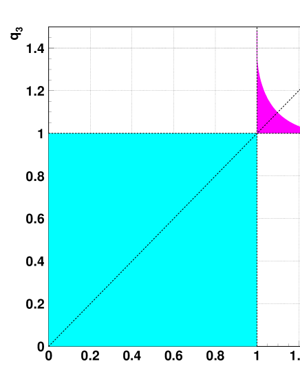
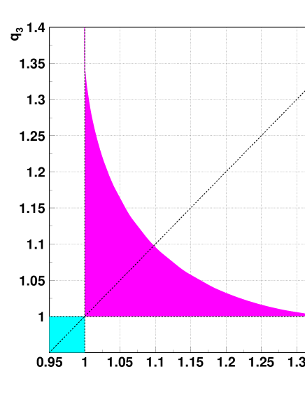
One expects an increase of stability near (T), where both thresholds become equal. This is what happens in the unit-charge case where, according to Hill’s theorem [5], we have stability for $\alpha_{2}=\alpha_{3}$. Another example is the Born–Oppenheimer limit with $m_{2}=m_{3}=\infty$, and say $m_{1}=q_{1}=1$ to fix the scales: in the $(q_{2},\,q_{3})$ plane, it is observed that the stability domain does not extend much beyond the unit square $(q_{2}\leq 1,\,q_{3}\leq 1)$, except for a spike around the $q_{2}=q_{3}$ axis, which reaches $q_{2}=q_{3}\simeq 1.24$ [6]. This is shown in Fig. 2.

Figure 2: Schematic shape of the stability domain in the Born–Oppenheimer limit. The heavy particles have charges $q_{2}$ and $q_{3}$. The charge of the light particle is set to $-q_{1}=-1$.

For fixed charged $q_{i}$, the triangular plot of Fig. 1 can be used again. The threshold separation (T) is a straight line passing through the (unphysical) point $\alpha_{1}=-1,\,\alpha_{2}=\alpha_{3}=1$, which is the mirror image of ${\rm A}_{1}$ with respect to ${\rm A}_{2}{\rm A}_{3}$. As seen in II, each instability domain remains star shaped and convex, as in the case of unit charges. In particular, if $q_{3}<q_{2}$ and $q_{3}<1$, the entire sub-triangle limited by (T) and ${\rm A}_{2}$ corresponds to stability. If furthermore $q_{2}<1$, then we have stability everywhere.

Following a suggestion by Gribov [7], one can also consider level lines of constant relative binding, i.e., such that

$$E_{12}^{(2)}<E_{13}^{(2)}\quad\hbox{and}\quad E^{(3)}/E_{12}^{(2)}=\lambda>1.$$ (6)

(Remember that both $E^{(3)}$ and $E_{12}^{(2)}$ are negative.) What happens is that the domain $E^{(3)}/E_{12}^{(2)}<\lambda$ (including the case where particle 3 is unbound, where we set $E^{(3)}=E_{12}^{(2)}$) is also convex and star shaped.

The proof is essentially the same as for the domain of instability. One first rescales the $\alpha_{i}$ from $\alpha_{1}+\alpha_{2}+\alpha_{3}=1$ to $\alpha_{1}+\alpha_{2}=1$, so that the threshold energy $E^{(2)}_{12}$ becomes constant. If two points $\vec{\alpha}=(\alpha_{1},\alpha_{2},\alpha_{3})$ and $\vec{\alpha}^{\prime}=(\alpha^{\prime}_{1},\alpha^{\prime}_{2},\alpha^{\prime}_{3})$ belong to the frontier of interest, that is to say

$$E^{(3)}(\vec{\alpha})=E^{(3)}(\vec{\alpha}^{\prime})=\lambda E_{12}^{(2)},$$ (7)

then as the $\alpha_{i}$ enter the Hamiltonian linearly, for any intermediate point $x\vec{\alpha}+(1-x)\vec{\alpha^{\prime}}$ with $0\leq x\leq 1$, one has

$$E^{(3)}(x\vec{\alpha}+(1-x)\vec{\alpha}^{\prime})\leq xE^{(3)}(\vec{\alpha})+(1-x)E^{(3)}(\vec{\alpha}^{\prime})=\lambda E_{12}^{(2)}.$$ (8)

Similarly, a decrease of $\alpha_{3}$ with $\alpha_{1}$ and $\alpha_{2}$ kept constant cannot do anything but decrease $E^{(3)}$ with $E^{(2)}_{12}$ unchanged: this proves the star-shape behaviour.

2.3 Convexity in the $q_{2}^{-1},q_{3}^{-1}$ variables

We return to the domain of strict instability, but now for fixed masses $m_{i}$ and variables charges. We fix $q_{1}=1$ and consider the frontier of stability in the ($1/q_{2},1/q_{3}$) plane.

First, we notice that the domain of stability is star-shaped with respect to the origin. Indeed, when a system of charges $(-1,q_{2},q_{3})$ is transformed into $(-1,q_{2}/\lambda^{2},q_{3}/\lambda^{2})$, with $\lambda>1$, the new system can be rescaled into $(-\lambda,q_{2}/\lambda,q_{3}/\lambda)$ which experiences the same attraction but less repulsion than the original system.

If $m_{2}<m_{3}$, the threshold separation (T) has a slope larger than unity in the ($1/q_{2},1/q_{3}$) plane. If $m_{2}>m_{3}$, this is the reverse. Consider now for definiteness the domain where

$$q_{2}^{2}\left(\alpha_{1}+\alpha_{3}\right)>q_{3}^{2}\left(\alpha_{1}+\alpha_{2}\right).$$ (9)

In this domain, the (1,2) atom is more bound than (1,3) and it is the energy of (1,2) to which $E^{(3)}$ should be compared. The ground-state energy $E^{(3)}$ of the Hamiltonian (2) is separately and globally concave in $q_{12}$, $q_{23}$ and $q_{23}$. With our choice of the charges we have

$$q_{12}=q_{2},\qquad q_{13}=q_{3},\qquad q_{23}=q_{2}q_{3},$$ (10)

but we can make a rescaling taking

$$\bar{q}_{12}=1,\qquad\bar{q}_{13}={q_{3}\over q_{2}},\qquad\bar{q}_{23}=q_{3}.$$ (11)

In this way, the binding energy of (1,2) is fixed. As $E^{(3)}$ is a concave function of $\bar{q}_{13}$ and $\bar{q}_{23}$, the instability domain is convex in the $(\bar{q}_{13},\bar{q}_{23})$ plane. This means a segment of straight line

$$\bar{q}_{13}=a\bar{q}_{23}+b$$ (12)

joining two points of the domain also belongs to the domain. But this equation translates into

$${1\over q_{2}}=a+b\left({1\over q_{3}}\right),$$ (13)

and thus also represents a straight line in the $(1/q_{2},1/q_{3})$ plane. Thus each instability domain is convex in this plane. This is schematically pictured in Fig. 3.

Figure 3: Shape of the stability domain in the plane of inverse charges $(q_{2}^{-1},q_{3}^{-1})$, with normalisation $q_{1}=1$. The lines $q_{2}^{-1}=1$ and $q_{2}^{-1}=1$ are either asymptotes, or part of the border, starting from a value of $q_{2}^{-1}$ or $q_{3}^{-1}$ which might be less than 1, unlike the case shown in this figure.

3 Instability of $(\alpha,p,\mu^{-})$ systems

The problem of the instability of ions such as $(\alpha,p,\mu^{-})$, $(\alpha,d,e^{-})$, etc., has been considered by several authors. What has been shown is essentially that, within the Born–Oppenheimer approximation, the effective $(\alpha,p)$ or $(\alpha,d)$ potential is unable to support a bound state [4]. The proof below is more general, for none of the masses is assumed to be very large.

First we notice that for equal charges $q_{2}=q_{3}>1.24$ [6] the 3-body system is unstable for equal masses $\alpha_{2}=\alpha_{3}$, because it is unstable for $\alpha_{2}=\alpha_{3}=0$ and $\alpha_{2}=\alpha_{3}=1/2$, and the domain of instability with respect to a given threshold is convex in the triangle of inverse masses.

Furthermore, using for instance the $(q_{2},q_{3})$ plane and keeping the masses equal and constant, we know that the system is unstable for a fixed $q_{2}>1.24$ and $q_{3}$ very small, because particle 3 is almost free and because the system (1,2) is repulsive. So using convexity in $q_{3}$ for fixed $q_{2}$, we prove that the system is unstable for $0<q_{3}<q_{2}$, if $q_{2}>1.24$, for $\alpha_{2}=\alpha_{3}$.

Therefore, if $\alpha_{2}=\alpha_{3}$, a system with $q_{2}=2$ and $q_{3}=1$ is unstable. But the system $(1,2)$ is repulsive and for $\alpha_{1}=\alpha_{2}=0$, i.e., $m_{1}=m_{2}=\infty$, we have instability. Now, in the left half-triangle $\alpha_{2}\leq\alpha_{3}$, where

$$(\alpha_{1}+\alpha_{3})q_{2}^{2}=4(\alpha_{1}+\alpha_{3})>(\alpha_{1}+\alpha_{2})q_{3}^{2}=\alpha_{1}+\alpha_{2},$$ (14)

so that it is the $(1,2)$ system which is more negatively bound. Therefore, we can use the star-shape instability in the whole left half-triangle, which includes not only $\alpha p\mu^{-}$ or $\alpha pe^{-}$, but also $\alpha d\mu^{-}$ or $\alpha t\mu^{-}$. Notice that the proof does not work for $q_{2}>q_{3}$, $m_{3}>m_{2}$.

4 Some limiting configurations

4.1 The very asymmetric Born–Oppenheimer case

In II the case was considered where the masses $m_{2}$ and $m_{3}$ are both infinite, but the corresponding charges $q_{2}$ and $q_{3}$ are freely varying. The stability domain is shown in Fig. 2, with a normalisation $q_{1}=1$. The domain is of course symmetric under $(q_{2}\leftrightarrow q_{3})$ exchange, and includes the $(q_{2}\leq 1,q_{3}\leq 1)$ unit square. We already mentioned the peak at $q_{2}=q_{3}\simeq 1.24$. The frontier starts from $q_{2}=1,q_{3}=0$, where a behaviour

$$q_{2}-1\simeq 18{q_{3}\over(-\ln q_{3})^{3}}.$$ (15)

is proved in II. This leading order (15) is however very crude, as the first corrections differ only by terms with higher power of $(-\ln q_{3})$.

4.2 The Born–Oppenheimer approximation for $m_{1}$ and $m_{2}$ very large, $q_{1}=q_{2}=1$

We now consider systems analogous to ($p,\bar{p},e^{-}$). In the limit of strictly infinite masses, we have a point source of charge $q_{2}-q_{1}$ acting on the charge $q_{3}>0$. Thus there is no binding if $q_{2}>q_{1}$ and binding for $q_{2}<q_{1}$. So, a non-trivial case consists of $m_{1}$ and $m_{2}$ very large but finite, and $q_{1}=q_{2}=1$. We argue below that binding is unlikely if $m_{3}q_{3}$ is very small.

With obvious notations, the adiabatic approximation relies on the decomposition

$$H=-{\Delta\over 2\mu_{12}}+h(r)-1/r$$

$$h=-{\Delta_{3}\over 2m_{3}}-{q_{3}\over r_{13}}+{q_{3}\over r_{23}}$$ (16)

with $\mu_{12}^{-1}=m_{1}^{-1}+m_{2}^{-1}$. Then $H\geq\tilde{H}$, where $\tilde{H}$ is deduced from $H$ by replacing $h$ by its ground-state energy or its infimum, say $\inf(h)$, which is a function of $r=r_{12}$.

The very crude inequality

$$r_{23}\leq r+r_{13}$$ (17)

leads to

$$h\geq-{\Delta_{3}\over 2m_{3}}-{q_{3}r\over r_{13}^{2}}.$$ (18)

As it is known that

$$-\Delta_{3}-{1\over 4r_{13}^{2}}>0,$$ (19)

we are sure that

$$h\geq 0\qquad\hbox{if}\qquad 8m_{3}q_{3}r<1.$$ (20)

On the other hand,

$$h\geq-{\Delta_{3}\over 2m_{3}}-{q_{3}\over r_{13}}\geq-{m_{3}q_{3}^{2}\over 2},$$ (21)

which is obtained for $r\to\infty$. So

$$\inf(h)\left\{\begin{array}[]{l@{\quad}l@{\quad}l}=0&\hbox{for}&r\leq(8m_{3}q_{3})^{-1}=R\\ \geq-m_{3}q_{3}^{2}/2&\hbox{for}&r>R.\\ \end{array}\right.$$ (22)

(Of course, $\inf h(r)$ must be a continuous function leaving 0 for some $r>R$, and reaching $-m_{3}q_{3}^{2}/2$ at large $r$.)

Consider now the relative motion as described by

$$\tilde{H}=-{\Delta\over 2\mu_{12}}+\inf(h)-{1\over r}.$$ (23)

If we neglect $\inf(h)$, $\tilde{H}$ reduces to the Schrödinger equation for a two-body atom, with ground-state energy $-\mu_{12}/2$ and reduced radial wave function $u(r)=2\mu_{12}^{3/2}r\exp(-\mu_{12}r)$. For $\mu_{12}\gg 1$, this wave function is concentrated near $r=0$ and $\inf(h)$ can be considered as a perturbation. The first order correction $\delta E$ is negative and is such that

$$|\delta E|\leq{m_{3}q_{3}^{2}\over 2}\int\limits_{R}^{\infty}u(r)^{2}\,{\rm d}r=\left[{\mu_{12}^{2}\over 64m_{3}}+{\mu_{12}q_{3}\over 8}+{m_{3}q_{3}^{2}\over 2}\right]\exp\left[-{\mu_{12}\over 4m_{3}q_{3}}\right].$$ (24)

In other words, $\delta E$ vanishes exponentially when $m_{1}$ and $m_{2}\to\infty$ for fixed $q_{3}$ and $m_{3}$. This is beyond the accuracy of the Born–Oppenheimer approximation, and strongly suggests that there is no binding if $m_{3}q_{3}\ll\mu_{12}$, which reduces, for $m_{1}=\infty$, to $m_{3}q_{3}\ll m_{2}$.

4.3 The small $m_{3}q_{3}$ limit for $m_{1}=\infty$

We now extend our study of the configurations with charges $q_{2}\gtrsim 1$ and $q_{3}\ll q_{2}$, with normalisation $q_{1}=1$. Instead of the Born–Oppenheimer limit, we consider the somewhat opposite case where $m_{1}=\infty$, i.e., the lower side ${\rm A}_{2}{\rm A}_{3}$ of the triangular plot. The threshold separation (T) happens for

$${\alpha_{3}\over\alpha_{2}}=\left({q_{3}\over q_{2}}\right)^{2},$$ (25)

very close to A₂. Some crude variational calculations has convinced us that the frontier occurs for $\alpha_{3}/\alpha_{2}={\cal O}(q_{3})$, not ${\cal O}(q_{3}^{2})$. This suggests a first order calculation in $q_{3}$. We temporarily fix the scale at $\alpha_{2}=1$ and split the Hamiltonian into

$$H = H_{0}+q_{3}H_{1},$$

$$H_{0} = -{1\over 2}\Delta_{2}-{q_{2}\over r_{2}},$$ (26)

$$H_{1} = -{1\over 2}\left({\alpha_{3}\over q_{3}}\right)\Delta_{3}-{1\over r_{3}}+{q_{2}\over r_{23}},$$

where $\vec{\rm r}_{1}=0$, and $r_{23}=|\vec{\rm r}_{3}-\vec{\rm r}_{2}|$. We are faced with a standard problem of degenerate perturbation theory. At zeroth order, we get the energy $E_{0}$ and eigenfunction $\Psi_{0}$

$$E_{0}=-{q_{2}^{2}\over 2},\qquad\Psi_{0}=\psi(\vec{\rm r}_{2})\varphi(\vec{\rm r}_{3}),$$ (27)

where $\psi(\vec{\rm r}_{2})=\pi^{-1/2}(q_{2})^{-3/2}\exp-(q_{2}r_{2})$ and $\varphi(\vec{\rm r}_{3})$, yet unspecified, is determined by diagonalising the restriction $\,\widetilde{\!H}_{1}$ of $H_{1}$ to the ground-state eigenspace of $H_{0}$. This reads

$$\,\widetilde{\!H}_{1}\varphi(\vec{\rm r}_{3}) = E_{1}\varphi(\vec{\rm r}_{3})$$

$$\,\widetilde{\!H}_{1} = -{1\over 2}\left({\alpha_{3}\over q_{3}}\right)\Delta_{3}-{1\over r_{3}}+{q_{2}\over r_{3}}f(q_{2}r_{3}),$$ (28)

$$f(x) = 1-(1+x)\exp(-2x).$$

For $q_{2}<1$, the potential in (4.3) exhibits an asymptotic Coulomb behaviour which is attractive. Thus $\,\widetilde{\!H}_{1}$ supports bound states whatever inverse mass $\alpha_{3}/q_{3}$ is involved. We recover the property seen in (II) that for $q_{3}<1$ and $q_{2}<1$, the 3-body system is stable for any choice of the constituent masses.

For $q_{2}\geq 1$, the potential in (4.3) has a repulsive Coulomb tail or decreases exponentially. At best, it offers a short-range pocket of attraction to trap the charge $q_{3}$. The short-range character is governed by the exponential in the form factor $f$, as per Eq. (4.3). Such a potential supports a bound state provided the mass $q_{3}/\alpha_{3}$ is large enough, say $q_{3}/\alpha_{3}>\mu_{c}$. This is why at the frontier $\alpha_{3}={\cal O}(q_{3})$.

Calculating the critical mass $\mu_{c}$ accurately as a function of $q_{2}$ is a routine numerical work. One can for instance integrate the radial equation at zero energy and look at whether or not a node occurs in the radial wave-function at finite distance. The result is shown in Fig. 4.

Figure 4: Minimal reduced mass $\mu_{c}$ to achieve binding in the potential $V=-1/r+q/r(1-(1+qr)\exp(-2qr))$.

The behaviour observed in Fig. 4 is not surprising. After rescaling, the Hamiltonian of Eq. (4.3) can be rewritten as

$$\,\widetilde{\!H}_{1}=2q^{2}\left[-{1\over\mu}{{\rm d}^{2}\over{\rm d}r^{2}}-\left({\exp(-r)\over r}+{\exp(-r)\over 2}\right)+{1-1/q\over r}\right]$$ (29)

where $q=q_{2}$ and $\mu=q_{3}/\alpha_{3}$. The critical mass for achieving binding in a Yukawa potential $V_{1}=-\exp(-r)/r$ is well known [8] and well studied [9]. It is $\mu_{1}\simeq 1.679$. For an exponential, it is about $1.446$ [8], and thus $\mu_{2}\simeq 2.892$ for $V_{2}=-\exp(-r)/2$. It is easily seen that the critical coupling $\mu_{c}$ for binding in $V_{1}+V_{2}$ is such $\mu_{c}^{-1}\leq\mu_{1}^{-1}+\mu_{2}^{-1}$. This means $\mu_{c}\geq 1.06$ for the the attractive part in (29), a bound not very far from the computed value $\mu_{c}\simeq 1.10$. This corresponds to the case $q=1$ in Fig. 4. For $q>1$, the repulsive Coulomb tail makes it necessary to use a larger value of $\mu_{c}$, this explaining the rise observed in Fig. 4.

4.4 Stability frontier for small $q_{3}/q_{2}$, and $q_{2}>1$

We just established that for $m_{1}=\infty$, small $q_{3}$, and $q_{2}>1$, the stability frontier lies at some $\alpha_{3}\simeq q_{3}/\mu_{c}$, where $\mu_{c}(q_{2})$ is computable from a simple radial equation. We now study how the frontier behaves as $m_{1}$ becomes finite. We are near A₂ in the triangle, where $\alpha_{2}\simeq 1$, and $\alpha_{1}$ and $\alpha_{3}$ are small.

We introduce the Jacobi variables

$$\vec{\rho}=\vec{\rm r}_{2}-\vec{\rm r}_{1},\quad\vec{\lambda}=\vec{\rm r}_{3}-{\alpha_{2}\vec{\rm r}_{1}+\alpha_{1}\vec{\rm r}_{2}\over\alpha_{1}+\alpha_{2}},$$ (30)

in terms of which the relative distances are

$$\vec{\rm r}_{12}=\vec{\rho},\quad\vec{\rm r}_{23}=\vec{\lambda}-{\alpha_{2}\over\alpha_{1}+\alpha_{2}}\vec{\rho},\quad\vec{\rm r}_{31}=-\vec{\lambda}-{\alpha_{1}\over\alpha_{1}+\alpha_{2}}\vec{\rho},$$ (31)

and the Hamiltonian reads

$$H= -{1\over 2}(\alpha_{1}+\alpha_{2})\Delta_{\rho}-{q_{2}\over\rho}-{1\over 2}\left(\alpha_{3}+{\alpha_{1}\alpha_{2}\over\alpha_{1}+\alpha_{2}}\right)\Delta_{\lambda}$$ (32)

$$-{q_{3}\over|\vec{\lambda}+\alpha_{1}\vec{\rho}/(\alpha_{1}+\alpha_{2})|}+{q_{2}q_{3}\over|\vec{\lambda}-\alpha_{2}\vec{\rho}/(\alpha_{1}+\alpha_{2})|},$$

besides the centre-of-mass motion, which will be now omitted.

A first rescaling $\vec{\rho}\rightarrow(\alpha_{1}+\alpha_{2})\vec{\rho}/\alpha_{2}$ results into

$$H= -{1\over 2}\left({\alpha_{2}^{2}\over\alpha_{1}+\alpha_{2}}\right)\Delta_{\rho}-{\alpha_{2}\over\alpha_{1}+\alpha_{2}}{q_{2}\over\rho}$$ (33)

$$-{1\over 2}\left(\alpha_{3}+{\alpha_{1}\alpha_{2}\over\alpha_{1}+\alpha_{2}}\right)\Delta_{\lambda}-{q_{3}\over|\vec{\lambda}+\alpha_{1}\vec{\rho}/\alpha_{2}|}+{q_{2}q_{3}\over|\vec{\lambda}-\vec{\rho}|},$$

which is the scale transformed of

$$\,\overline{\!H}=-{1\over 2}\bar{\alpha}_{2}\Delta_{2}-{1\over 2}\bar{\alpha}_{3}\Delta_{3}-{\bar{q}_{2}\over r_{2}}+{\bar{q}_{2}\bar{q}_{3}\over r_{23}}-{\bar{q}_{3}\over|\vec{\rm r}_{3}+\alpha_{1}\vec{\rm r}_{2}/\alpha_{2}|},$$ (34)

provided the inverse masses in $\,\overline{\!H}$ are proportional to these in $H$, and the strengths in $\,\overline{\!H}$ to these of $H$. A convenient rule of transformation of masses is

$$\bar{\alpha}_{2} = {1\over\alpha_{2}+\alpha_{3}}\left({\alpha_{2}^{2}\over\alpha_{1}+\alpha_{2}}\right)$$

$$\bar{\alpha}_{3} = {1\over\alpha_{2}+\alpha_{3}}\left(\alpha_{3}+{\alpha_{1}\alpha_{2}\over\alpha_{1}+\alpha_{2}}\right),$$ (35)

since it changes our triangular normalisation $\sum\alpha_{i}=1$ into $\bar{\alpha}_{2}+\bar{\alpha}_{3}=1$.

For the charges, the simultaneous identification

$$\bar{q}_{2} = Cq_{2}{\alpha_{2}\over\alpha_{1}+\alpha_{2}},$$

$$\bar{q}_{3} = Cq_{3},$$ (36)

$$\bar{q}_{2}\bar{q}_{3} = Cq_{3}q_{2},$$

results into

$$\bar{q}_{2}=q_{2},\qquad\bar{q}_{3}=q_{3}{\alpha_{1}+\alpha_{2}\over\alpha_{2}}.$$ (37)

The rescaled Hamiltonian (34) slightly differs from the Hamiltonian (4.3) corresponding to $m_{1}=\infty$. However, the difference between $|\vec{\rm r}_{3}+\alpha_{1}\vec{\rm r}_{2}/\alpha_{2}|$ and $r_{3}$ is of first order in $q_{3}$, and thus enters at order $q_{3}^{2}$ in $\,\overline{\!H}$. We are then allowed to write the frontier condition as in the previous section, namely

$$\bar{\alpha}_{3}\simeq{\bar{q}_{3}\over\mu_{c}},$$ (38)

which, when translated into the original variables, reads, at first order

$$\alpha_{1}+\alpha_{3}\simeq{q_{3}\over\mu_{c}},$$ (39)

to be compared with the threshold separation $\alpha_{1}+\alpha_{3}=q_{3}^{2}$. This means the frontier is at first approximation a straight line, parallel to the side A₃A₁ of the triangle of inverse masses, as schematically pictured in Fig. 5.

Figure 5: Expected behaviour of the frontier (F) in a situation where $q_{2}>1$ and the ratio $q_{3}/q_{2}$ is very small, so that the threshold separation (T) is very close to A₂.

Note that the actual frontier is certainly curved, since the instability domains are convex, as reminded in Sec. 2.

4.5 The small $q_{3}$ limit in the $(q_{2},q_{3})$ plane

Let us consider now the $(q_{2},q_{3})$ plane (with $q_{1}=1$) for fixed masses. The shape of the stability domain is shown in Fig. 6.

Figure 6: Shape of the stability domain in the $(q_{2},q_{3})$ plane. The frontier of stability leaves the vertical side $q_{2}=1$ of the unit square at some finite value of $q_{3}$. It also leaves the horizontal line $q_{3}=1$ at some finite value of $q_{2}$, which can either smaller (as in this figure) or larger than 1.

The frontier of stability leaves the unit square at some finite value of $q_{3}$. Consider, indeed, $q_{2}=1$, with $\alpha_{1}=0$ for simplicity, and a mass scale fixed at $\alpha_{2}=1$. In a (variational) approximation of a (1,2) atom times a function describing the motion of the third particle, we can read the calculation of Sec. 4.3 as

$$1>q_{3}>\mu_{c}(1)\alpha_{3}\simeq 1.10\alpha_{3}$$ (40)

being a sufficient condition for stability.

A necessary condition of the same type, i.e., $q_{3}>\tilde{\mu}_{c}\alpha_{3}$ can be obtained using the method of Glaser et al. [10]. The decomposition

$$H=\left(H-{q_{2}q_{3}\over r_{23}}\right)+{q_{2}q_{3}\over r_{23}}$$ (41)

yields the operator inequality [11]

$$H\geq H^{\prime}=\left(H-{q_{2}q_{3}\over r_{23}}\right)+q_{2}q_{3}P(P\,r_{23}\,P)^{-1}P,$$ (42)

where $P$ is the projector over the ground-state of $H_{0}=-\Delta_{2}-q_{2}/r_{2}$ (times the identity in the variable $\vec{\rm r}_{3}$). Now $H^{\prime}$ is the sum of $H_{0}$ in the variable $\vec{\rm r}_{2}$, and

$$H^{\prime}_{0}=-\alpha_{3}\Delta_{3}-q_{3}/r_{3}+{q_{2}q_{3}\over r_{3}}\left[1-{x^{2}\over 1-(1+x/2)\exp(-2x)}\right]^{-1},$$ (43)

where $x=q_{2}r_{3}$, in the variable $\vec{\rm r}_{3}$. For $q_{2}=1$, this potential supports a bound-state provided $q_{3}>\tilde{\mu}_{c}\alpha_{3}$, with $\tilde{\mu}_{c}>0.34$ from the Jost–Pais–Bargmann rule [12], and $\tilde{\mu}_{c}\simeq 0.64$ from a numerical calculation (looking for nodes in the radial wave function at zero energy).

If $\alpha_{1}>0$, a reasoning similar to that of Subsec. 4.4 shows that the sufficient condition (40) is replaced by

$$q_{3}>\mu_{c}(1)(\alpha_{1}+\alpha_{3})\simeq 1.10(\alpha_{1}+\alpha_{3}),$$ (44)

where the normalisation is $\alpha_{1}+\alpha_{2}+\alpha_{3}=1$.

The result (44) is of course expected to be better if the computed $q_{3}$ is small, i.e., if $\alpha_{1}+\alpha_{3}\ll 1$.

4.6 Frontier in the $(q_{2},q_{3})$ plane at small $\alpha_{3}/\alpha_{2}$

We remain in the $(q_{2},q_{3})$ plane for fixed masses. We assume $\alpha_{1}=0$ for simplicity, but some results do not depend on this assumption. We can normalise to $\alpha_{2}=1$. In the limit where $\alpha_{3}$ is small, the threshold separation (T), as given by Eq. (25), has a very small slope with respect to the $q_{3}$ axis.

The frontier exits out of the unit square at $q_{2}=1$ and a finite value of $q_{3}$ which is close to $\alpha_{3}\mu_{c}(1)$, where $\mu_{c}(1)\simeq 1.10$, according to our previous computation. If we look at the frontier outside the unit square, we have two questions:

• in the lower part of the plot, is the frontier strictly below (T) ?

• in the upper part, does the frontier overcome the line $q_{3}=1$ ?

4.6.1 Lower part of the frontier

To answer the first question, let us consider a situation where $q_{3}$ is close to but smaller than 1, and thus $q_{2}\sim\alpha_{3}^{-1/2}$ is large. If particles 2 and 3 would ignore each other, they would bind around particle 1 with approximately the same energy, since we are close to (T), but with different Bohr radii $R_{i}$, namely $R_{3}/R_{2}\sim\alpha_{3}^{1/2}\ll 1$. This suggests the approximation of a localised (1,3) source attracting the charge $q_{2}$, corresponding to a 3-body energy

$$E_{3}=-{q_{3}^{2}\over\alpha_{3}}-q_{2}^{2}(1-q_{3})^{2},$$ (45)

whose equality with the threshold $E_{2}=-q_{2}^{2}$ gives the approximate frontier

$$q_{2}^{2}={1\over\alpha_{3}}{q_{3}\over 2-q_{3}}$$ (46)

which just touches (T) at $q_{3}=1$, as seen in Fig. 7.

Figure 7: Upper bound (46) on the lower part of the stability frontier, touching the threshold separation (T) for $q_{3}=1$. A value $\alpha_{3}/\alpha_{2}=1/25$ is assumed here. Note that this bound is not expected to be a good approximation for small $q_{2}$, as it does not delimit a convex domain of instability.

Now this approximation corresponds to write a decomposition

$$H = H_{23}+V_{23}$$ (47)

$$= \left[{\alpha_{3}\over 2}\vec{\rm p}_{3}^{2}-{q_{3}\over r_{3}}+{1\over 2}\vec{\rm p}_{2}^{2}-{q_{2}(1-q_{3})\over r_{2}}\right]+q_{2}q_{3}\left({1\over r_{23}}-{1\over r_{2}}\right),$$

and neglect the second term, $V_{23}$. The spherically-symmetric ground-state $\Psi_{0}$ of $H_{23}$ can be chosen as a trial variational wave-function for $H$. The Gauss theorem implies that $\langle\Psi_{0}|V_{23}|\Psi_{0}\rangle<0$. Hence the ground state of $H$ lies below that of $H_{23}$, and the actual frontier is below the approximation (46), therefore below (T) as long as $q_{3}<1$.

4.6.2 Upper part

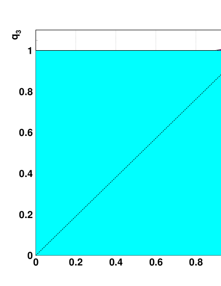
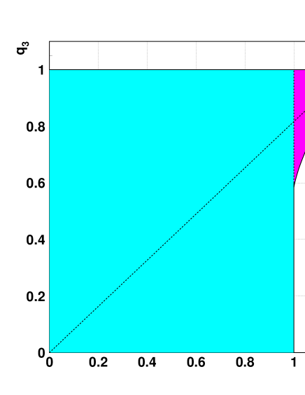
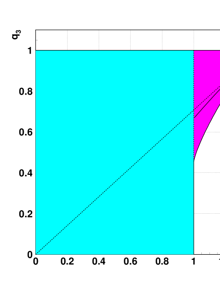
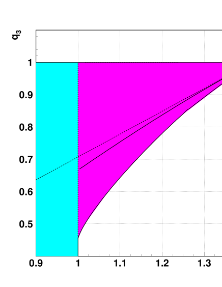
We now turn to the question of possible binding above the line $q_{3}=1$. We restrict ourselves to $m_{1}=\infty$, although we suspect that our results are more general. Numerical investigations using the method described in Appendix B suggest the following pattern. For $m_{2}=m_{3}$, a spike is observed on the diagonal. It reaches about $q_{2}=q_{3}=1.24$ in Fig. 2, corresponding to $m_{2}=m_{3}=\infty$, and about $q_{2}=q_{3}=1.098$ [13] for $m_{2}=m_{3}\ll m_{1}$. The spike remains for moderate values of the mass ratio $m_{3}/m_{2}$, as schematically shown in Fig. 6. When, however, $m_{3}/m_{2}$ exceeds a value which is about 1.8, no spike is seen within the accuracy of our calculations, i.e., the frontier seemingly coincides with the line $q_{3}=1$, until it reaches (T), as pictured in Fig. 8.

We are able to show rigorously below that, for large values of $m_{3}/m_{2}$ no binding occurs above $q_{3}=1$ for $q_{2}\leq(3/4)^{1/2}(m_{3}/m_{2})^{1/2}$. Nothing can be said however from this latter value to $q_{2}=(m_{3}/m_{2})^{1/2}$ on the threshold separation (T). In other words, a very tiny peak along (T) overcoming $q_{3}=1$ cannot be excluded.

Figure 8: Schematic shape of the stability domain in the $(q_{2},q_{3})$ plane, for the limiting case where $\alpha_{3}/\alpha_{2}$ is very small. Our constraints cannot exclude a very tiny peak along (T) above $q_{3}=1$.

For $m_{1}=\infty$ and $q_{3}=1$, the Hamiltonian reduces to

$$H = \left[{\vec{\rm p}_{3}^{2}\over 2m_{3}}-{1\over r_{3}}\right]+{\vec{\rm p}_{2}^{2}\over 2m_{2}}-{q_{2}\over r_{2}}+{q_{2}\over r_{23}}$$ (48)

$$= H_{0}+{\vec{\rm p}_{2}^{2}\over 2m_{2}}-{q_{2}\over r_{2}}+{q_{2}\over r_{23}}.$$

Let $P$ be the projector on $\Phi(r_{3})$, the ground state of $H_{0}={\vec{\rm p}_{3}^{2}/(2m_{3})}-{1/r_{3}}$, and $\Psi$ the ground state of $H$. We have the inequality

$$\left(\int{\rm d}\vec{\rm r}_{3}\Psi{1\over r_{23}}\Psi\right)\left(\int{\rm d}\vec{\rm r}_{3}\Phi\,r_{23}\,\Phi\right)\geq\left(\int{\rm d}\vec{\rm r}_{3}\Psi\Phi\right)^{2}=\left(P\Psi(\vec{\rm r}_{2})\right)^{2}.$$ (49)

To estimate $\langle\Psi|H|\Psi\rangle$, we first need $\langle\Psi|H_{0}|\Psi\rangle$, where each $\Psi$ can be read as $P\Psi+(1-P)\Psi$. We have

$$\langle\Psi P|H_{0}|(1-P)\Psi\rangle=0,$$

$$\langle\Psi P|H_{0}|P\Psi\rangle=\langle\Psi P|P\Psi\rangle\,(-{m_{3}/2}),$$ (50)

$$\langle\Psi(1-P)|H_{0}|(1-P)\Psi\rangle\geq\langle\Psi(1-P)|(1-P)\Psi\rangle\,(-{m_{3}/8}),$$

and similarly, for $h_{0}={\vec{\rm p}_{2}^{2}/(2m_{2})}-{q_{2}/r_{2}}$,

$$\langle\Psi P|h_{0}|(1-P)\Psi\rangle=0,$$ (51)

$$\langle\Psi(1-P)|h_{0}|(1-P)\Psi\rangle\geq\langle\Psi(1-P)|(1-P)\Psi\rangle\,(-q_{2}^{2}{m_{2}/2}).$$

Thus

$$\langle\Psi|H|\Psi\rangle\geq |\!|P\Psi|\!|^{2}\left(-{m_{3}\over 2}\right)+\langle\Psi P|\tilde{h}_{0}|P\Psi\rangle$$ (53)

$${}+|\!|(1-P)\Psi|\!|^{2}\left[-{m_{3}\over 8}-{q_{2}^{2}m_{2}\over 2}\right],$$

where

$$\tilde{h}_{0}={\vec{\rm p}_{2}^{2}/(2m_{2})}-{q_{2}/r_{2}}+{q_{2}\over\int\Phi^{2}\,r_{23}\,{\rm d}\vec{\rm r}_{2}}.$$ (54)

In a situation where $\tilde{h}_{0}$ does not support any bound state,

$$\langle\Psi|H|\Psi\rangle>|\!|P\Psi|\!|^{2}\left(-{m_{3}\over 2}\right)+|\!|(1-P)\Psi|\!|^{2}\left[-{m_{3}\over 8}-{q_{2}^{2}m_{2}\over 2}\right],$$ (55)

and hence

$$\langle\Psi|H|\Psi\rangle>\inf\left\{\begin{array}[]{l}-m_{3}/2\\ -m_{3}/8-m_{2}q_{2}^{2}/2.\end{array}\right.$$ (56)

Now the hamiltonian $\tilde{h}_{0}$ has been studied in Ref. [10], and shown not to bind if

$${2m_{2}q_{2}\over m_{3}}<1.2706.$$ (57)

Therefore if

$$-{m_{3}\over 2}<-{m_{3}\over 8}-{m_{2}q_{2}^{2}\over 2},\qquad\hbox{and}\qquad{2m_{2}q_{2}\over m_{3}}<1.2706,$$ (58)

the system is unstable (the first condition implies $-m_{3}/2<-m_{2}q_{2}^{2}/2$, i.e., (1,3) is the lowest threshold). For large $m_{3}/m_{2}$, the first condition is more constraining, so we have no stability above $q_{3}=1$ from $q_{2}=0$ to $q_{2}=(3m_{3}/(4m_{2}))^{1/2}$.

4.7 Numerical results

We now display an estimate of the domain of stability in the $(q_{2},\,q_{3})$ plane, with normalisation $q_{1}=1$. The method, described in Appendix B, is variational. Therefore, the approximate domain drawn here is included in the true domain.

Our investigations correspond to $m_{1}=\infty$, and the mass ratio $m_{3}/m_{2}$ having the values 1, 1.1, 1.5 and 2. In each case, we show the whole domain, and an enlargement of its most interesting part, the spike above $q_{2}=1$ and $q_{3}=1$.

                                               

Figure 9: Variational estimate of the domain of stability for $m_{1}=\infty$ and $m_{2}/m_{3}=1$, full view (left) and enlargement of the spike (right). The dotted line is the threshold separation (T).

                                               

Figure 10: Same as Fig. 9, for $m_{2}/m_{3}=1.1$

                                               

Figure 11: Same as Fig. 9, for $m_{2}/m_{3}=1.5$

                                               

Figure 12: Same as Fig. 9, for $m_{2}/m_{3}=2$. The dotted curve below (T) corresponds to the crude approximation of Eq. (46).

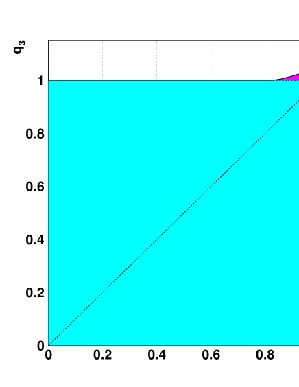
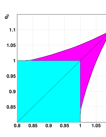
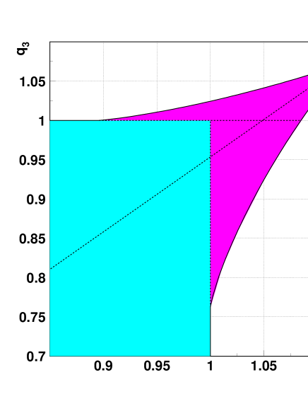
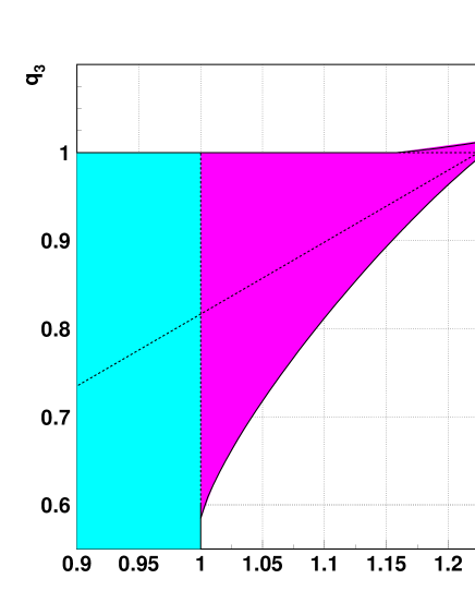
For $m_{2}=m_{3}$, in Fig. 9, we have a symmetric spike. The location of the peak at, $q_{2}=q_{3}=1.098$ reproduces fairly well the values given in the literature [13].

For $m_{2}/m_{3}=1.1$, in Fig. 10, the spike leaves the horizontal line $q_{3}=1$ before $q_{2}=1$, as a generalized H^- ion with unit charges and masses $(\infty,\,1.1,\,1)$ is bound. This is no longer the case for $m_{2}/m_{3}=1.5$, as seen in Fig. 11.

For $m_{2}/m_{3}=2$, shown in Fig. 12, the domain found in our variational calculation is flat. In the lower part, it extends appreciably further than indicated by the crude approximation of Eq. (46).

5 Outlook

Many questions remain open concerning the stability of 3-charge systems. Along the paper, we pointed out that in some limiting cases, more accurate results would be desirable. For instance, a question is whether very large values of the mass ratio $m_{3}/m_{2}$ exclude the possibility of binding with $q_{3}>1$.

There are also more general questions, concerning domains of some parameters for which stability will never be reached, whatever value is given to the other parameters.

For given masses $m_{i}$, the answer is immediate: there is always a set of charges, for instance $q_{3}<q_{2}<q_{1}=1$, that makes the system stable.

For given charges $q_{2}$ and $q_{3}$, and $q_{1}=1$ to fix the scale, the situation is different: one has clearly three possibilities. Region {1} is the unit square $\{q_{2}<1,\,q_{3}<1\}$, where any mass configuration corresponds to a stable ion. Region {2} includes for instance the point $q_{2}=2$ and $q_{3}=0.8$: there is sometimes stability, $m_{1}=\infty$, $m_{2}\ll m_{3}$ is an example, and sometimes breaking into an atom and a charge, as for $m_{1}=\infty$, $m_{2}\gg m_{3}$. Region {3} includes points like $q_{2}=q_{3}=2$ for which stability will never occur. Determining the properties of the boundary between regions {2} and {3} would be very interesting.

A possible starting point is the result by Lieb [14], that for a fixed nucleus $\alpha_{1}=0$, $q_{1}=1$, a bound state will never occur if

$${1\over q_{2}}+{1\over q_{3}}<1.$$ (59)

A simple proof is given in Appendix A.

This upper bound for possible stability at $m_{1}=\infty$ (i.e., stability occurring for at least some value of $m_{2}/m_{3}$) is not too far from the lower bound of Fig. 13, obtained from our variational method. More extensive computations would be necessary to sketch the shape of the domain of absolute instability, in particular by relaxing the condition $m_{1}=\infty$. Note that along the symmetry axis, the limit is $q_{2}=q_{3}\simeq 1.098$ for $m_{1}=\infty$ and $m_{2}=m_{3}$ finite, while it reaches $q_{2}=q_{3}\simeq 1.24$ for $m_{1}$ finite and $m_{2}=m_{3}=\infty$. Thus, along the symmetry axis, the frontier between regions {2} and {3} is saturated in the Born–Oppenheimer limit. On the other hand, for $q_{2}\gg q_{3}$ or $q_{2}\ll q_{3}$, the question is whether this frontier has $q_{2}=1$ and $q_{3}=1$ as actual asymptotes, as tentatively pictured in Fig.14 or reached these lines above some values of $q_{2}$ or $q_{3}$.

                                               

Figure 13: Variational estimate of the domain of possible stability beyond $q_{2}=1$ and $q_{3}=1$, for $m_{1}=\infty$. Inside the domain, stability occurs at least for some value of the mass ratio $m_{2}/m_{3}$.

Figure 14: Guess at the shape of the border of the domain of absolute instability. In region {1}, binding occurs for any set of constituent masses. In region {2}, binding is achieved under some conditions for the masses. In region {3}, stability is never obtained.

Appendix A:
Proof of instability for $q_{2}^{-1}+q_{3}^{-1}<1$

We give here a proof of the result on instability for all values of $m_{2}$ and $m_{3}$ if $q_{2}^{-1}+q_{3}^{-1}<1$, provided $\alpha_{1}=0$, with normalization $q_{1}=1$.

First, it is shown that $r\vec{\rm p}^{2}$ is a positive operator, in the sense that any diagonal matrix element is positive. Indeed, separating the radial and angular part of $\vec{\rm p}^{2}$,

$$\langle\Psi|r\vec{\rm p}^{2}|\Psi\rangle = -\int r\Psi\Delta\Psi\,{\rm d}^{(3)}\vec{\rm r}$$ (60)

$$= \int r\Psi{L^{2}\over r^{2}}\Psi\,{\rm d}^{(3)}\vec{\rm r}-\int{\rm d}\Omega\int\left[r\Psi{\partial^{2}(r\Psi)\over\partial r^{2}}\right]r{\rm d}r$$

$$= \int r\left|\overrightarrow{\nabla}_{\Omega}\Psi\right|^{2}+\int{\rm d}\Omega\int r{\rm d}r\left({\partial(r\Psi)\over\partial r}\right)^{2}$$

$$= \int{{\rm d}^{(3)}\vec{r}\over r}\left|\overrightarrow{\nabla}(r\Psi)\right|^{2}.$$

Now consider the Hamiltonian

$$H={\vec{\rm p}_{2}^{2}\over 2m_{2}}+{\vec{\rm p}_{3}^{2}\over 2m_{3}}-{q_{2}\over r_{2}}-{q_{3}\over r_{3}}+{q_{2}q_{3}\over r_{23}},$$ (61)

whose thresholds $(1,i)$ with $i=2,3$ are governed by the Hamiltonian

$$h_{i}={\vec{\rm p}_{i}^{2}\over 2m_{i}}-{q_{i}\over r_{i}}.$$ (62)

These $h_{i}$ and the 3-body Hamiltonian $H$ fulfill the identity

$${r_{3}}(H-h_{2})+{r_{2}}(H-h_{3})={r_{2}}{\vec{\rm p}_{2}^{2}\over 2m_{2}}+{r_{3}}{\vec{\rm p}_{3}^{2}\over 2m_{3}}+q_{2}q_{3}\left({r_{2}+r_{3}\over r_{23}}-{1\over q_{2}}-{1\over q_{3}}\right).$$ (63)

In the r.h.s., the two first terms are always positive, and so is the third one if $q_{2}^{-1}+q_{3}^{-1}<1$, due to the triangular inequality. Looking now at the l.h.s., its expectation value is always positive, which means that

$$\langle\Psi|r_{3}(H-h_{2})|\Psi\rangle>0\quad\hbox{or}\quad\langle\Psi|r_{2}(H-h_{3})|\Psi\rangle>0.$$ (64)

In the first case take $\Psi$ as the ground state of $H$, which satisfies $H\Psi=E^{(3)}\Psi$. This translates into

$$E^{(3)}\langle\Psi|r_{3}|\Psi\rangle>\langle\Psi|r_{3}\left({\vec{\rm p}_{2}^{2}\over 2m_{2}}-{q_{2}\over r_{2}}\right)|\Psi\rangle,$$ (65)

or

$$E^{(3)}\langle\sqrt{r}_{3}\Psi|\sqrt{r}_{3}\Psi\rangle>\langle\sqrt{r}_{3}\Psi|\left({\vec{\rm p}_{2}^{2}\over 2m_{2}}-{q_{2}\over r_{2}}\right)|\sqrt{r}_{3}\Psi\rangle\geq E^{(2)}_{12}\langle\sqrt{r}_{3}\Psi|\sqrt{r}_{3}\Psi\rangle$$ (66)

from the variational principle. In the second case

$$E^{(3)}>E^{(2)}_{13}$$ (67)

So, if $m_{1}=\infty$ and $q_{2}q_{3}>q_{2}+q_{3}$, either $E^{(3)}>E^{(2)}_{12}$ or $E^{(3)}>E^{(2)}_{13}$.

Appendix B: Variational method

We briefly describe the variational method used for the numerical results displayed in this paper. More details can be found in [15]. The ground state of the Hamiltonian (2) has been searched using trial wave functions of the type [16]

$$\Psi=\sum_{i}C_{i}\varphi_{i}=\sum_{i}C_{i}\left[\exp(-a_{i}r_{23}-b_{i}r_{31}-c_{i}r_{12})+\cdots\right]$$ (68)

from which all matrix elements can be calculated in close form. The dots are meant for similar terms obtained by permutation, in the case of identical particles. For given range parameters, the weights $C_{i}$ are listed in a vector $\mathbf{C}$, which is found, together with the variational energy $\epsilon$, from the matrix equation

$$\left(\widetilde{T}+\widetilde{V}\right)\mathbf{C}=\epsilon\widetilde{N}\mathbf{C},$$ (69)

involving the restrictions of the kinetic and potential energy to the space spanned by the $\varphi_{i}$, whose scalar products are stored in the positive-definite matrix $\widetilde{N}$.

As the number of terms increases, it quickly becomes impossible to determine the best range parameters, even with powerful minimization programs, as too many neighboring sets give comparable energies. One way out [17] consists of imposing all $a_{i},\,b_{i}$ and $c_{i}$ to be taken in a geometric series. Then only the smallest and the largest have to be determined numerically. For instance, this method allows one to reproduce the binding energy $-0.262005$ of the Ps^- ion, in agreement with the best results in the literature.

The question now is to find the frontier. Let us consider, for instance, the problem of Sec. 4.6.2. Here $m_{1}=\infty$, $q_{1}=m_{2}=1$, and $q_{2}/q_{3}=m_{3}^{1/2}$ when one searches the limit of stability among the threshold separation (T).

One can estimate the ground-state energy of

$${\vec{\rm p}_{2}^{2}\over 2}+{\vec{\rm p}_{3}^{2}\over 2m_{3}}-{m_{3}^{1/2}q_{3}\over r_{2}}-{q_{3}\over r_{3}}+{m_{3}^{1/2}q_{3}^{2}\over r_{23}},$$ (70)

starting from some low value of $q_{3}$, and examine, by suitable interpolation, for which $q_{3}$ it matches the threshold $E_{\rm the}=-q_{3}^{2}m_{3}/2$.

A more direct strategy consists to set $E=E_{\rm the}$ in the Schrödinger equation, apply a rescaling and solve

$${\vec{\rm p}_{2}^{2}\over 2}+{\vec{\rm p}_{3}^{2}\over 2m_{3}}-{m_{3}^{1/2}\over r_{2}}-{1\over r_{3}}+{m_{3}\over 2}=-q_{3}\,{m_{3}^{1/2}\over r_{23}},$$ (71)

using the same trial function (68), resulting in a matrix equation very similar to (69), where the positive-definite matrix $\widetilde{N}$ now represents the restriction of $m_{3}^{1/2}/r_{23}$ in the space of the $\varphi_{i}$. In principle, the variational wave function needs not to be normalizable at threshold, but this becomes immaterial as soon as very long range components are introduced in the expansion (68). It was checked that the extrapolation method and the direct computation give the same result for the frontier.

References

- [1] A. Martin, J.-M. Richard and T.T. Wu, Phys. Rev. A43 (1992) 3697.
- [2] A. Martin, J.-M. Richard and T.T. Wu, Phys. Rev. A52 (1995) 2557.
- [3] For a review, see, for instance, E.A.G. Armour and W. Byers Brown, Accounts of Chemical Research, 26 (1993) 168.
- [4] Z. Chen and L. Spruch, Phys. Rev. A 42 (1990) 133, and references therein.
- [5] R.N. Hill, J. Math. Phys. 18 (1977) 2316.
- [6] H. Hogreve, J. Chem. Phys. 98 (1993) 5579.
- [7] V.N. Gribov, private communication.
- [8] J.M. Blatt and A.D. Jackson, Phys. Rev. 76 (1949) 18.
- [9] O.A. Gomes, H. Chacham, and J.R. Mohallem, Phys. Rev. A50 (1994) 228.
- [10] V. Glaser, H. Grosse, A. Martin and W. Thirring, in Studies in Mathematical Physics, Essays in Honor of Valentine Bargmann, eds. A.S. Wightmann, E.H. Lieb and B. Simon (Princeton University Press, Princeton, 1976).
- [11] W. Thirring, A Course in Mathematical Physics, Vol. 3: Quantum Mechanics of Atoms and Molecules (Springer Verlag, New-York, 1979), p. 156.
- [12] R. Jost and A. Pais, Phys. Rev. 82 (1951) 840; V. Bargmann, Proc. Nat. Ac. Sci. (US) 38 (1952) 961.
- [13] J.D. Baker, D.E. Freund, R.N. Hill, and J.D. Morgan, Phys. Rev. A41 (1990) 1247; I.A. Ivanov, Phys. Rev. A51 (1995) 1080; A52 (1995) 1942.
- [14] E. Lieb, Phys. Rev. A 29 (1984) 3018.
- [15] A. Krikeb, Thèse, Université Claude Bernard, Lyon, 1998.
- [16] E.A. Hylleraas, Z. Phys. 54 (1929) 347; S. Chandrasekhar, Astr. J. 100 (1944) 176.
- [17] M. Kamimura, Phys. Rev. A 38 (1988) 621; H. Kameyama, M. Kamimura and Y. Fukushima, Phys. Rev. C 40 (1989) 974.