Abstract

We calculate the pair correlation function of an interacting Bose gas in a harmonic trap directly via Path Integral Quantum Monte Carlo simulation for various temperatures and compare the numerical result with simple approximative treatments. Around the critical temperature of Bose-Einstein condensation, a description based on the Hartree-Fock approximation is found to be accurate. At low temperatures the Hartree-Fock approach fails and we use a local density approximation based on the Bogoliubov description for a homogeneous gas. This approximation agrees with the simulation results at low temperatures, where the contribution of the phonon-like modes affects the long range behavior of the correlation function. Further we discuss the relation between the pair correlation and quantities measured in recent experiments.
PACS numbers: 03.75.Fi, 02.70.Lq, 05.30.Jp

I Introduction

One of the appealing features of the experimental achievement of Bose-Einstein condensation in dilute vapors [1, 2, 3], is the demonstration of first order coherence of matter waves [4]. The interference pattern of this experiment agrees with the theoretical calculation [5], which reveals that the underlying theoretical concept of off-diagonal long range order due to a macroscopically occupied quantum state is justified [6]. Additional experiments have explored certain aspects of second and third order coherence of a trapped Bose gas [7, 8, 9]. Here we study the density-density correlation function which is related to second order coherence. With the knowledge of this pair correlation function, the total interaction energy can be calculated. In [7] the release energy of the atoms was measured after switching off the magnetic trap. In the Thomas Fermi regime at zero temperature the initial kinetic energy can be neglected and the release energy is dominated by the interaction energy. By comparison with the usual mean field interaction energy using a contact potential, it was concluded that the release energy is mainly proportional to the pair correlation function at vanishing relative distance. Strictly speaking this statement cannot be correct as for interactions with a repulsive hard core the pair correlation function must vanish at zero distance. To give a precise meaning to this statement one needs to access the whole correlation function.

In this paper we consider in detail the spatial structure of the correlation function of an interacting trapped Bose gas. The Fourier transform of this function is directly related to the static structure factor which can be probed by off-resonant light scattering. The tendency of bosonic atoms to cluster together causes atom-bunching for an ideal gas above the condensation temperature, for the atoms separated by less than the thermal de-Broglie wavelength [10]. For the condensate atoms, this bunching vanishes, since they all occupy the same quantum state [11, 12]. However, for a gas with strong repulsive interatomic interaction, it is impossible to find two atoms at exactly the same place, and hence the pair correlation function must vanish at very short distances. This mutual repulsion can significantly reduce the amount of bosonic bunching at temperatures around the transition temperature [13]. At much lower temperature, the presence of the condensate changes the excitation spectrum as compared to the noninteracting case. It is known that in a homogeneous Bose gas the modes of the phonons give rise to a modification of the long range behavior of the correlation function [14].

Using path integral quantum Monte Carlo simulations all equilibrium properties of Bose gases can be directly computed without any essential approximation [15]. It has been shown that this calculation can be performed directly for the particle numbers and temperatures of experimental interest [16]. Here, we use this approach to calculate the pair correlation function for various temperatures and compare our results with simple approximate treatments.

Near the critical temperature our data are quantitatively well explained by an improved semiclassical Hartree-Fock theory, where the full short range behavior is taken into account. At low temperature this single-particle approximation fails since the low lying energy modes become important and they are not correctly described by the Hartree-Fock treatment. In the Bogoliubov approach these modes are phonon-like and change the behavior of the correlation function. Adapting the homogeneous Bogoliubov solution locally to the inhomogeneous trap case we find an excellent agreement with the Monte Carlo simulation results at low temperature.

II Hamiltonian of the problem

The Hamiltonian of $N$ interacting particles in an isotropic harmonic trap with frequency $\omega$ is given by

$$H=\sum_{i=1}^{N}\left[\frac{p_{i}^{2}}{2m}+\frac{1}{2}m\omega^{2}r_{i}^{2}\right]+\frac{1}{2}\sum_{i\neq j}V(r_{ij}),$$ (1)

where $V$ is the interatomic potential, which depends only on the relative distance $r_{ij}=|\vec{r}_{i}-\vec{r}_{j}|$ between two particles. This potential in the experiments with alkali atoms has many bound states, so that the Bose-condensed gases are metastable systems rather than systems at thermal equilibrium. To circumvent this theoretical difficulty, we have to replace the true interaction potential by a model potential with no bound states.

This model potential is chosen in a way that it has the same low energy binary scattering properties as the true interaction potential. In the considered experiments, the $s$-wave contribution strongly dominates in a partial wave expansion of the binary scattering problem, so that it is sufficient that the model potential have the same $s$-wave scattering length $a$ as the true potential. For simplicity we take in the quantum Monte Carlo calculations a pure hard-core potential with diameter $a$. In the analytical approximations of this paper, we have taken, as commonly done in the literature, the pseudo-potential described in [14], which is a regularized form of the contact potential, $g\delta(\vec{r}_{1}-\vec{r}_{2})\frac{\partial}{\partial r_{12}}(r_{12}\cdot)$, with a coupling constant

$$g={4\pi\hbar^{2}a\over m}.$$ (2)

III Path Integral Quantum Monte Carlo Approach

A Reminder of the Method

The partition function $Z$ of the system with inverse temperature $\beta=(k_{B}T)^{-1}$ is given as the trace over the (unnormalized) density matrix $\varrho$:

$$\varrho(\beta)=e^{-\beta H}$$ (3)

over all symmetrized states. Both satisfy the usual convolution equation which we can write in the position representation:

$$Z = \frac{1}{N!}\sum_{P}\int\,d^{3N}R\,\varrho(R,R^{P},\beta)$$ (4)

$$= \frac{1}{N!}\sum_{P}\int\,d^{3N}R\,\int\,d^{3N}R_{2}\,...\int\,d^{3N}R_{M}\,\varrho(R,R_{2},\tau)...\varrho(R_{M},R^{P},\tau).$$ (5)

Here $\tau=\beta/M$, where $M$ is an arbitrary integer, $R$ is the 3N-dimensional vector of the particle coordinates $R=(\vec{r}_{1},\vec{r}_{2},...,\vec{r}_{N})$, $P$ is a permutation of the $N$ labels of the atoms and $R^{P}$ denotes the vector with permuted labels: $R^{P}=(\vec{r}_{P(1)},\vec{r}_{P(2)},...,\vec{r}_{P(N)})$. Since only density matrices at higher temperature ($\tau\ll\beta$) are involved, high temperature approximations of the $N$-body density matrix can be used.

The simplest approximation is the primitive approximation corresponding to $\exp[\tau(A+B)]\simeq\exp[\tau B/2]\exp[\tau A]\exp[\tau B/2]$, which neglects the commutator of the operators $A$ and $B$. It corresponds to a discrete approximation of the Feynman-Kac path integral and gives the correct result in the limit $M\rightarrow\infty$ [17, 15]. This can be seen by using the Trotter formula for the exponentials of a sum of two noncommuting operators

$$e^{\tau(A+B)}=\lim_{n\to\infty}\left(e^{\tau A/n}e^{\tau B/n}\right)^{n}.$$ (6)

The discretisized path integral for the $N$-particle density matrix at inverse temperature $\tau$ can therefore be written in the primitive approximation with symmetric splitting as

$$\varrho(R,R^{\prime},\tau)\simeq\prod_{k=1}^{N}\varrho_{1}(\vec{r}_{k},\vec{r}_{k}\,^{\prime},\tau)\prod_{i<j}\exp\left[-\frac{\tau}{2}\left(V(\vec{r}_{ij})+V(\vec{r}_{ij}\,^{\prime})\right)\right],$$ (7)

where $\varrho_{1}(\vec{r}_{k},\vec{r}_{k}\,^{\prime},\tau)$ is the density matrix of noninteracting particles in the harmonic trap and $\vec{r}_{ij}=\vec{r}_{i}-\vec{r}_{j}$, $\vec{r}\,^{\prime}_{ij}=\vec{r}\,^{\prime}_{i}-\vec{r}\,^{\prime}_{j}$. However, this approximation leads to slow convergence since the potential energy in the argument of the exponentials are not slowly varying compared to the density matrix of one particle in the external potential, $\varrho_{1}(\vec{r}_{i},\vec{r}_{i}\,^{\prime},\tau)$. This has the consequence that eq.(7) is not a smooth function in the region where two particles are in contact, as it should. In order to get such a smooth function we use the fact that the potential energy part of eq.(7) can also be written as:

$$e^{-\tau\left(V(\vec{r}_{ij})+V(\vec{r}_{ij}\,^{\prime})\right)/2}\simeq g_{2}(\vec{r}_{ij};\vec{r}_{ij}\,^{\prime},\tau)=\left\langle e^{-\int_{0}^{\tau}d\,t\,V(\vec{r}_{ij}(t))}\right\rangle_{rw},$$ (8)

where the brackets correspond an average over an arbitrary distribution of $\vec{r}_{ij}(t)$, starting from $\vec{r}_{ij}$ and ending at $\vec{r}_{ij}\,^{\prime}$, which reproduces the correct high temperature limit of the primitive approximation. It is convenient to take the random walk corresponding to the kinetic energy as weight function so that $g_{2}$ is the solution of the binary scattering problem in free space:

$$g_{2}(\vec{r}_{ij},\vec{r}\,^{\prime}_{ij};\tau)=\frac{\langle\vec{r}_{ij}|\exp[-\tau(p_{ij}^{2}/m+V(r_{ij}))]|\vec{r}\,^{\prime}_{ij}\rangle}{\langle\vec{r}_{ij}|\exp[-\tau p_{ij}^{2}/m]|\vec{r}\,^{\prime}_{ij}\rangle},$$ (9)

where $\vec{p}_{ij}$ is the operator of the relative momentum between particles $i$ and $j$. This leads to the so called pair-product approximation [18, 15], where the density matrix is approximated as

$$\varrho(R,R^{\prime},\tau)\simeq\prod_{n=1}^{N}\varrho_{1}(\vec{r}_{n},\vec{r}_{n}\,^{\prime},\tau)\prod_{i<j}g_{2}(\vec{r}_{ij};\vec{r}_{ij}\,^{\prime},\tau).$$ (10)

This approximation has the advantage to include exactly all binary collisions of atoms in free space, only three and more atoms in close proximity will lead to an error; convergency with respect to $M\rightarrow\infty$ is reached much faster. In the simulation the two-particle correlation function $g_{2}$ is equal to one for non-interacting particles and plays the role of a binary correction term in presence of two-body interactions.

As in [16] we take $N=10,000$ particles with a hard-core radius of $a=0.0043(\hbar/m\omega)^{1/2}$. The transition temperature of the noninteracting Bose-gas is $k_{B}T_{c}^{0}=20.26\,\hbar\omega$ or $\beta_{c}^{0}\simeq 0.05(\hbar\omega)^{-1}$ and a value of $\tau=0.01(\hbar\omega)^{-1}$ was found sufficient. In the low temperature regime ($k_{B}T\ll\hbar^{2}/ma^{2}$) the most important contribution to $g_{2}$ for hard spheres is the $s$-wave contribution, which can be calculated analytically [19]; for non vanishing relative angular momenta ($l>0$) we neglect the effect of the potential outside of the hard core. In this way we can obtain an explicit formula for $g_{2}$,

$$g_{2}(\vec{r},\vec{r}\,^{\prime};\tau)=1+\left({\hbar^{2}\beta\over m}\right){1\over rr^{\prime}}\left\{\exp\left[-{(r+r^{\prime})^{2}\over 4\hbar^{2}\beta/m}\right]-\exp\left[-{(r+r^{\prime}-2a)^{2}\over 4\hbar^{2}\beta/m}\right]\right\}e^{-(rr^{\prime}+\vec{r}\cdot\vec{r}\,^{\prime})m/2\hbar^{2}\beta}$$ (11)

for $\vec{r}$ and $\vec{r}\,^{\prime}$ outside of the hard core diameter ($|\vec{r}|>a$ and $|\vec{r}\,^{\prime}|>a$), otherwise $g_{2}=0$.

The density-density correlation function can be easily calculated as

$$\varrho^{(2)}(\vec{r}\,^{\prime};\vec{r}\,^{\prime\prime},\beta)=\sum_{i}\sum_{j\neq i}\langle\delta(\vec{r}\,^{\prime}-\vec{r}_{i})\delta(\vec{r}\,^{\prime\prime}-\vec{r}_{j})\rangle.$$ (12)

As the atoms are in a trap rather than in free space, this quantity is not a function of the relative coordinates $\vec{r}\,^{\prime}-\vec{r}\,^{\prime\prime}$ of the two particles only. Imagine however that this pair distribution function be probed experimentally by scattering of light by the atomic gas, where we assume a large beam waist compared to the atomic sample. As the Doppler effect due to the atomic motion is negligible, the scattering cross section depends only on the spatial distribution of the atoms. Furthermore, for a weak light field very far detuned from the atomic transitions, the scattering cross section can be calculated in the Born approximation; it then depends only on the distribution function of the relative coordinates $\vec{r}\,^{\prime}-\vec{r}\,^{\prime\prime}$ between pairs of atoms. We therefore take the trace over the center-of-mass position $\vec{R}=(\vec{r}\,^{\prime}+\vec{r}\,^{\prime\prime})/2$:

$$\varphi^{(2)}(r,\beta)\equiv\frac{1}{N(N-1)}\int\,d^{3}\vec{R}\,\varrho^{(2)}(\vec{R}+\vec{r}/2;\vec{R}-\vec{r}/2,\beta),$$ (13)

where we have divided by the number of pairs of atoms to normalize $\varphi^{(2)}$ to unity. Note that the result depends only on the modulus $r$ of $\vec{r}$ as the trapping potential is isotropic.

B Results of the Simulation

In fig.1 we show $\varphi^{(2)}(r,\beta)$ for various temperatures below $T_{c}^{0}$, obtained by the simulation of the interacting bosons in the harmonic trap, where the critical temperature $T_{c}$ is reduced compared to the ideal gas [20, 16, 21]. All pair correlation functions are zero in the region of the hard-core radius as they should. At larger length scales the $r$ dependence of the result is also simple to understand qualitatively, as we discuss now.

Consider first the case $T>T_{c}$, where no condensate is present. As the typical interaction energy $n(r)g$ ($n(r)$ being the total one-particle density at $\vec{r}$) is much smaller than $k_{B}T$, we expect to recover results close to the ideal Bose gas. The size of the thermal cloud $(k_{B}T/m\omega)^{1/2}$ determines the spatial extent of $\varphi^{(2)}(r)$; the bosonic statistics leads to a spatial bunching of the particles with a length scale given by the thermal de Broglie wavelength

$$\lambda_{T}=\sqrt{\frac{2\pi\hbar^{2}}{mk_{B}T}}.$$ (14)

The Bose enhancement of the pair distribution function is maximal and equal to a factor of 2 for particles at the same location ($\vec{r}=0$). This effect is preserved by the integration over the center of mass variable and manifests itself through a bump on $\varphi^{(2)}(r)$ in fig.1. Due to the influence of interactions the bump is suppressed at small distances and the factor of 2 is not completely obtained.

For $T<T_{c}$ a significant fraction of the particles accumulate in the condensate. As the size of the condensate is smaller than that of the thermal cloud, the contribution to $\varphi^{(2)}$ of the condensed particles has a smaller spatial extension, giving rise to wings with two spatial components in $\varphi^{(2)}$, as seen in fig.1. Apart from this geometrical effect the building up of a condensate also affects the bosonic correlations at the scale of $\lambda_{T}$: The bosonic bunching at this scale no longer exists for particles in the condensate. This property, referred to as a second order coherence property of the condensate [7, 8, 13], is well understood in the limiting case $T=0$; neglecting corrections due to interactions, all the particles are in the same quantum state $|\psi_{0}\rangle$ so that e.g. the 2-body density matrix factorizes in a product of one-particle pure state density matrices. This reveals the absence of spatial correlations between the condensed particles. This explains why in fig.1 the relative height of the exchange bump with respect to the total height is reduced when $T$ is lowered, that is when the number of non-condensed particles is decreased.

IV Comparison with simple approximate treatments

At this stage a quantitative comparison of the Quantum Monte Carlo results with well known approximations can be made.

A In presence of a significant thermal cloud: Hartree-Fock approximation

As shown in [21] in detail, at temperatures sufficiently away from the critical temperature, the Hartree-Fock approximation [20] gives a very good description of the thermodynamic one-particle properties.

To derive the Hartree-Fock Hamiltonian we start from the second quantized form of the Hamiltonian with contact potential

$$\hat{H}=\int\,d^{3}\vec{r}\,\left[\hat{\Psi}^{\dagger}(\vec{r})(H_{0}-\mu)\hat{\Psi}(\vec{r})\;+\;\frac{g}{2}\,\hat{\Psi}^{\dagger}(\vec{r})\hat{\Psi}^{\dagger}(\vec{r})\hat{\Psi}(\vec{r})\hat{\Psi}(\vec{r})\right]$$ (15)

where $H_{0}$ is the single particle part of the Hamiltonian. Due to the presence of the condensate we split the field operator $\hat{\Psi}$ in a classical part $\psi_{0}$, corresponding to the macroscopically occupied ground state and the part of the thermal atoms $\hat{\psi}$ with vanishing expectation value $\langle\hat{\psi}\rangle=0$:

$$\hat{\Psi}(\vec{r})\simeq\psi_{0}(\vec{r})+\hat{\psi}(\vec{r}).$$ (16)

After this separation we make a “quadratization” of the Hamiltonian by replacing the interaction term by a sum over all binary contractions of the field operator, keeping one or two operators uncontracted, e.g.

$$\hat{\psi}^{\dagger}\hat{\psi}^{\dagger}\hat{\psi}\hat{\psi}\simeq 4\langle\hat{\psi}^{\dagger}\hat{\psi}\rangle\hat{\psi}^{\dagger}\hat{\psi}-2\langle\hat{\psi}^{\dagger}\hat{\psi}\rangle\langle\hat{\psi}^{\dagger}\hat{\psi}\rangle.$$ (17)

This is done in such a way that the mean value of the right hand side agrees with the mean value of the left hand side in the spirit of Wick’s theorem. In the Hartree-Fock approximation we neglect the anomalous operators, such as $\hat{\psi}^{\dagger}\hat{\psi}^{\dagger}$, and their averages, and we end up with a Hamiltonian which is quadratic in $\psi_{0}$ and $\hat{\psi}$, but also linear in $\hat{\psi}$ and $\hat{\psi}^{\dagger}$. Now we choose $\psi_{0}$ such that these linear terms vanish in order to force $\langle\hat{\psi}\rangle=0$. This gives the Gross-Pitaevskii equation for the condensate [22]

$$\left\{-\frac{\hbar^{2}\nabla^{2}}{2m}+\frac{1}{2}m\omega^{2}r^{2}+g[n_{0}(r)+2n_{T}(\vec{r},\vec{r})]\right\}\psi_{0}(r)=\mu\psi_{0}(r)$$ (18)

where $n_{0}(r)=|\psi_{0}(r)|^{2}$ corresponds to the condensate density with $N_{0}$ particles and $n_{T}(\vec{r},\vec{r})=\langle\hat{\psi}^{\dagger}(\vec{r})\hat{\psi}(\vec{r})\rangle$ is the density of the thermal cloud.

Up to a constant term we are left with the Hamiltonian for the thermal atoms

$$\hat{H}=\int\,d^{3}\vec{r}\,\hat{\psi}^{\dagger}(\vec{r})(H_{0}+2gn(r)-\mu)\hat{\psi}(\vec{r})$$ (19)

where $n(r)=n_{0}(r)+n_{T}(\vec{r},\vec{r})$ denotes the total density and depends only on the modulus of $\vec{r}$. To work out the density-density correlation function, we formulate (12) in second quantization:

$$\varrho^{(2)}(\vec{r};\vec{r}\,^{\prime},\beta)=\langle\hat{\Psi}^{\dagger}(\vec{r})\hat{\Psi}^{\dagger}(\vec{r}\,^{\prime})\hat{\Psi}(\vec{r}\,^{\prime})\hat{\Psi}(\vec{r})\rangle,$$ (20)

we use the splitting (16), together with Wick’s theorem and get

$$\varrho^{(2)}_{HF}(\vec{r};\vec{r}\,^{\prime},\beta) = \psi_{0}(r)\psi_{0}(r)\psi_{0}(r^{\prime})\psi_{0}(r^{\prime})$$ (23)

$$+\psi_{0}(r)\psi_{0}(r)n_{T}(\vec{r}\,^{\prime},\vec{r}\,^{\prime})+\psi_{0}(r^{\prime})\psi_{0}(r^{\prime})n_{T}(\vec{r},\vec{r})+2\psi_{0}(r)\psi_{0}(r^{\prime})n_{T}(\vec{r},\vec{r}\,^{\prime})$$

$$+n_{T}(\vec{r},\vec{r})n_{T}(\vec{r}\,^{\prime},\vec{r}\,^{\prime})+n_{T}(\vec{r},\vec{r}\,^{\prime})n_{T}(\vec{r},\vec{r}\,^{\prime}).$$

Here we have chosen the condensate wave function to be real and

$$n_{T}(\vec{r},\vec{r}\,^{\prime})=\langle\hat{\psi}^{\dagger}(\vec{r})\hat{\psi}(\vec{r}\,^{\prime})\rangle$$ (24)

corresponds to the nondiagonal elements of the thermal one body density matrix. Since the Hamiltonian (19) of the thermal atoms is quadratic in $\hat{\psi}$, this density matrix is given by

$$n_{T}(\vec{r},\vec{r}\,^{\prime})=\langle\vec{r}|\frac{1}{\exp{[\beta(H_{0}+2gn(r)-\mu)]}-1}|\vec{r}\,^{\prime}\rangle.$$ (25)

In the semiclassical approximation ($k_{B}T\gg\hbar\omega$) we can calculate explicitly these matrix elements by using the Trotter break-up, which neglects the commutator of $r$ and $p$:

$$n_{T}(\vec{r},\vec{r}\,^{\prime}) = \sum_{l=1}^{\infty}\langle\vec{r}|e^{-l\beta(\frac{p^{2}}{2m}+\frac{1}{2}m\omega^{2}r^{2}+2gn(r)-\mu)}|\vec{r}\,^{\prime}\rangle$$ (26)

$$\simeq \sum_{l=1}^{\infty}e^{-\frac{l\beta}{2}\left(\frac{1}{2}m\omega^{2}r^{2}+2gn(r)-\mu\right)}\,\langle\vec{r}|e^{-l\beta\frac{p^{2}}{2m}}|\vec{r}\,^{\prime}\rangle\,e^{-\frac{l\beta}{2}\left(\frac{1}{2}m\omega^{2}r^{\prime 2}+2gn(r^{\prime})-\mu\right)}.$$ (27)

We finally get

$$n_{T}(\vec{r},\vec{r}\,^{\prime})=\frac{1}{\lambda_{T}^{3}}\sum_{l=1}^{\infty}\frac{1}{l^{3/2}}\left(\exp\left[-\pi\frac{|\vec{r}-\vec{r}\,^{\prime}|^{2}}{l\lambda_{T}^{2}}-l\beta\left(m\omega^{2}(r^{2}+r^{\prime 2})/4+g(n(r)+n(r^{\prime}))-\mu\right)\right]\right).$$ (28)

For the diagonal elements the summation gives immediatly the Bose function $g_{3/2}(z)=\sum_{l=1}^{\infty}z^{l}/l^{3/2}$. For a given number of particles $N$, eq.(18) and the diagonal elements $\vec{r}=\vec{r}\,^{\prime}$ of eq.(28) have to be solved self consistently to get the condensate density $n_{0}(r)$ and the thermal cloud $n_{T}(\vec{r},\vec{r})$. With this solution we can work out the nondiagonal matrix elements of the density operator which give rise to the exchange contribution of the density-density correlation (23), and the correlation function can be written as a sum over the direct and the exchange contribution

$$\varrho^{(2)}_{HF}(\vec{r};\vec{r}\,^{\prime},\beta)=\varrho^{(2)}_{direct}(\vec{r};\vec{r}\,^{\prime},\beta)+\varrho^{(2)}_{exchange}(\vec{r};\vec{r}\,^{\prime},\beta).$$ (29)

Up to now the short range correlations due to the hard core repulsion have not been taken into account, but we can improve the Hartree-Fock scheme further to include the fact that it is impossible to find two atoms at the same location: We assume that the particle at $\vec{r}$ interacts with the full Hamiltonian with the particle at $\vec{r}\,^{\prime}$ but only with the mean-field of all others (over which we integrated to derive the reduced density matrix). This gives in first approximation:

$$\widetilde{\varrho}^{(2)}_{HF}(\vec{r};\vec{r}\,^{\prime},\beta) = \varrho^{(2)}_{direct}(\vec{r};\vec{r}\,^{\prime},\beta)g_{2}(\vec{r}-\vec{r}\,^{\prime};\vec{r}-\vec{r}\,^{\prime},\beta)+\varrho^{(2)}_{exchange}(\vec{r};\vec{r}\,^{\prime},\beta)g_{2}(\vec{r}-\vec{r}\,^{\prime};\vec{r}\,^{\prime}-\vec{r},\beta)$$ (30)

$$\simeq \varrho^{(2)}_{HF}(\vec{r};\vec{r}\,^{\prime},\beta)g_{2}(\vec{r}-\vec{r}\,^{\prime};\vec{r}-\vec{r}\,^{\prime},\beta)$$ (31)

where the two particle correlation function $g_{2}$ is the solution of the binary scattering problem, eq.(11). Further we used the fact that $g_{2}\simeq 1$ for particle distances of the order of $\lambda_{T}$ and larger. In principle one should integrate over the second particle to get a new one-particle density matrix and find a self-consistent solution of the Hamiltonian. But since the range of $g_{2}$ is of the order of the thermal wavelength, it will only slightly affect the density, so we neglect this iteration procedure. Using the solution of the coupled Hartree-Fock equations to calculate (31), and integrating over the center-mass-coordinate, we get $\varphi_{HF}^{(2)}(r,\beta)$. As shown in fig.1, this gives a surprisingly good description of the correlation function at high and intermediate temperatures.

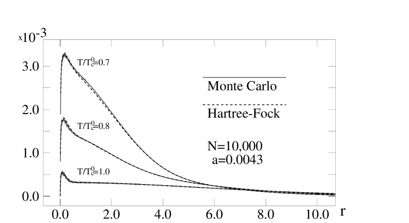
FIG. 1.: Pair correlation function $\varphi^{(2)}(r,\beta)$ vs $r$ in units of the harmonic oscillator length $(\hbar/m\omega)^{1/2}$ from the Monte-Carlo and the Hartree-Fock calculations for $\beta=0.05(\hbar\omega)^{-1}$, $\beta=0.06(\hbar\omega)^{-1}$, and $\beta=0.07(\hbar\omega)^{-1}$ (from the bottom to the top). The corresponding condensate fractions $N_{0}/N$ are $0.0$ ($T/T_{c}^{0}\simeq 1.0$), $0.22$ ($T/T_{c}^{0}\simeq 0.8$), and $0.45$ ($T/T_{c}^{0}\simeq 0.7$). $T_{c}^{0}$ is the Bose-Einstein condensation temperature for the ideal gas. For clarity we removed the part of short $r$ for the upper curves.

B The quasi-pure condensate: Bogoliubov approach

The Hartree-Fock description must fail near zero temperature: Since the anomalous operators $\hat{\psi}^{\dagger}\hat{\psi}^{\dagger}$ and $\hat{\psi}\hat{\psi}$ have been neglected, it describes not well the low energy excitations of the systems. It is known that the zero temperature behavior can be well described by the Bogoliubov approximation [23]. In this paper it is not our purpose to calculate the correlation function using the complete Bogoliubov approach in the inhomogeneous trap potential. This could be performed using approaches developed in [24, 25]. Here we use the homogeneous description of the Bogoliubov approximation and adapt it to the inhomogeneous trap case with a local density approximation. This approach already includes the essential features which the Hartree-Fock description neglects at low temperatures.

We start with the description of the homogeneous system with quantization volume $V$ and uniform density $n=N/V$. As in [26] we split the field operator $\hat{\Psi}$ into a macroscopically populated state $\Phi$ and a remainder, which accounts for the noncondensed particles:

$$\hat{\Psi}(r)=\Phi(r)\hat{a}_{\Phi}+\delta\hat{\Psi}(r).$$ (32)

In the thermodynamic limit $N\rightarrow\infty$, $V\rightarrow\infty$, keeping $N/V=n$ and $Ng=const$, the typical matrix elements of $\delta\hat{\Psi}$ at low temperatures are $\sqrt{N}$ times smaller than $\hat{a}_{\Phi}$. Hence we can neglect terms cubic and quartic in $\delta\hat{\Psi}$, when we insert (32) in the expression of the density-density correlation function (20). Since the condensate density is given by the total density minus the density of the excited atoms, we have to express the operator of the condensate density in the same order of approximation for consistency,

$$\hat{a}_{\Phi}^{\dagger}\hat{a}_{\Phi}=\hat{N}-\frac{1}{N}\int\,d^{3}r\,\delta\hat{\Psi}^{\dagger}(r)\hat{a}_{\Phi}\hat{a}_{\Phi}^{\dagger}\delta\hat{\Psi}(r)+O(N^{-1/2}).$$ (33)

Finally we use the mode decomposition of the homogeneous system

$$\frac{1}{\sqrt{N}}\hat{a}_{\Phi}^{\dagger}\delta\hat{\Psi}(r)=\frac{1}{\sqrt{V}}\sum_{\vec{k}\neq 0}\left[\hat{b}_{\vec{k}}e^{i\vec{k}\cdot\vec{r}}u_{k}+\hat{b}^{\dagger}_{\vec{k}}e^{-i\vec{k}\cdot\vec{r}}v_{k}^{*}\right]$$ (34)

where $\hat{b}_{\vec{k}}$ annihilates a quasiparticle with momentum $\vec{k}$. The components $u_{k}$ and $v_{k}$ satisfy the following equations:

$$\left(\begin{array}[]{cc}\frac{\hbar^{2}k^{2}}{2m}+gn&gn\\ -gn&-\left(\frac{\hbar^{2}k^{2}}{2m}+gn\right)\end{array}\right)\left(\begin{array}[]{c}u_{k}\\ v_{k}\end{array}\right)=E_{k}\left(\begin{array}[]{c}u_{k}\\ v_{k}\end{array}\right)$$ (41)

together with the normalization:

$$|u_{k}|^{2}-|v_{k}|^{2}=1.$$ (42)

At low temperatures the quasiparticles have negligible interactions and we can use Wick’s theorem to get the following expression for the correlation function

$$\varrho_{BG}(\vec{r}\,^{\prime};\vec{r}\,^{\prime\prime},\beta)=n^{2}+2n\int\,d^{3}k\,e^{i\vec{k}\cdot(\vec{r}\,^{\prime}-\vec{r}\,^{\prime\prime})}\left[(u_{k}^{2}+v_{k}^{2}+2u_{k}v_{k})\langle\hat{b}_{\vec{k}}^{\dagger}\hat{b}_{\vec{k}}\rangle+v_{k}^{2}+u_{k}v_{k}\right]+O(\sqrt{n})$$ (43)

where we used $\Phi(r)=V^{-1/2}$. The quasiparticles obey Bose statistics, so that the mean number of quasiparticles with momentum $\vec{k}$ and energy $E_{k}$ is given by

$$\langle\hat{b}_{\vec{k}}^{\dagger}\hat{b}_{\vec{k}}\rangle=\frac{1}{e^{\beta E_{k}}-1}.$$ (44)

We see from eq.(43) that in the homogeneous system the density-density correlation function depends only on the relative distance $r=|\vec{r}\,^{\prime}-\vec{r}\,^{\prime\prime}|$. The derivation of the properties of the pair correlation function is given in the appendix. At $T=0$ the pair correlation function has the following behavior [14, 27]

$$\varphi_{n=const}^{(2)}(r,T=0)\simeq\left\{\begin{array}[]{cc}\frac{1}{V}\left[1-\frac{2a}{r}\right]\simeq\frac{1}{V}\left[1-\frac{a}{r}\right]^{2}&(r\ll\xi)\\ &\\ \frac{1}{V}\left[1-16\sqrt{\frac{na^{3}}{\pi}}\left(\frac{\xi}{r}\right)^{4}\right]&(r\gg\xi)\end{array}\right.$$ (48)

where $\xi=(8\pi na)^{-1/2}$ is the healing length of the condensate. For finite but small temperatures this structure is only slightly changed (see appendix). The modification of the low energy spectrum due to the Bogoliubov approach is responsible for the long range part of the correlation function.

Apart from the edge of the condensate, the total density $n(r)$ for low temperature in the trapped system varies rather slowly compared to the healing length $\xi$ for the considered parameters. So it is possible to adapt the result of the homogeneous system to the inhomogeneous trap case. For a given density $n(r)$ we get with a local density approximation for the pair correlation function instead of eq.(43)

$$\varphi_{BG}^{(2)}(r,\beta) \simeq \int\,d^{3}\vec{R}\,\left\{n(|\vec{R}+\vec{r}/2|)n(|\vec{R}-\vec{r}/2|)\right.$$ (50)

$$+2n(R)\left.\int\,d^{3}k\,e^{i\vec{k}\cdot\vec{r}}\left[(u_{k}^{2}(R)+v_{k}^{2}(R)+2u_{k}(R)v_{k}(R))\left(e^{\beta E_{k}(R)}-1\right)^{-1}+v_{k}^{2}(R)+u_{k}(R)v_{k}(R)\right]\right\}$$

where $u_{k}(R)$, $v_{k}(R)$, and $E_{k}(R)$ are solutions of eq.(41) for the given density $n(R)$.

As shown in fig.2 this gives an excellent agreement with the Quantum Monte Carlo results at low temperature. We have checked that at this temperature the difference with the Bogoliubov solution at $T=0$ is almost negligible. The good agreement with the simulation reflects that the long range behavior of the pair correlation function in this approximation is correctly described by eq.(48). We note that in an intermediate temperature regime, which is not shown, both approaches, the Hartree-Fock and the local density Bogoliubov calculation, do not reproduce the simulation results quantitatively: The maximum local error is about $5\%$.

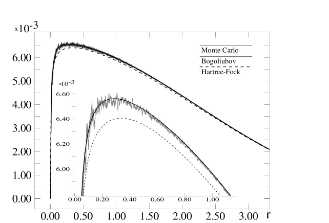
FIG. 2.: Pair correlation function $\varphi^{(2)}(r,\beta)$ vs $r$ in units of the harmonic oscillator length $(\hbar/m\omega)^{1/2}$ from the Monte Carlo, the Bogoliubov and the Hartree-Fock calculations for $\beta=0.20(\hbar\omega)^{-1}$ with a condensate fraction $N_{0}/N\simeq 0.95$ ($T/T_{c}^{0}\simeq 0.25$). The healing length is roughly $\xi\simeq 0.3$ in this units

V Connection to the interaction energy

The knowledge of the pair correlation function permits us to calculate the total energy of the trapped atoms $E_{tot}$:

$$E_{tot}=\frac{1}{\mbox{Tr}\{\rho\}}\left[\mbox{Tr}\{H_{0}\rho\}+\mbox{Tr}\{H_{I}\rho\}\right]$$ (51)

One has to pay attention that the regularized form of the contact potential, $V=g\delta(\vec{r})\frac{\partial}{\partial r}\left(r\cdot\right)$, acts on the off-diagonal elements $r_{12}$ and $r_{12}^{\prime}$ of the density-density correlation function $\varphi(r_{12}^{\prime},r_{12},\beta)=\langle\vec{r}_{1}\,^{\prime},\vec{r}_{2}\,^{\prime}|\rho|\vec{r}_{1},\vec{r}_{2}\rangle$ in the space of relative coordinates $r_{12}$ and $r_{12}^{\prime}$. As the 2-body density matrix $\varphi(r_{12}^{\prime},r_{12},\beta)$ diverges as $(1-a/r_{12}^{\prime})(1-a/r_{12})$ we actually get the simple form:

$$\frac{1}{\mbox{Tr}\{\rho\}}\mbox{Tr}\{H_{I}\rho\} = \frac{N(N-1)g}{4}\int\,d\vec{r}\frac{\delta(\vec{r})}{r}\frac{\partial}{\partial r}\left(r^{2}\varphi^{(2)}(r,\beta)\right).$$ (52)

This form involves only the diagonal elements of the correlation function $\varphi^{(2)}(r,\beta)$. Both the improved Hartree-Fock solution and the Bogoliubov solution behave for small distances ($r\ll\xi$) like

$$\varphi^{(2)}(r\simeq 0,\beta)\simeq(1-a/r)^{2}\widetilde{\varphi}^{(2)}(0,\beta)$$ (53)

where $\widetilde{\varphi}^{(2)}(0,\beta)$ can be obtained graphically by extrapolating the pair correlation function to zero, neglecting the short range behavior ($r<\xi$); numerically it can be obtained from the Hartree-Fock calculation of (23) (see [13] for analysis of the temperature dependence of $\widetilde{\varphi}^{(2)}(0,\beta)$ ). This behavior of the correlation functions shows that eq.(52) gives a finite contribution linear in $a$, which we can identify with the mean interaction energy $\langle H_{I}\rangle$:

$$\langle H_{I}\rangle\simeq g\frac{N(N-1)}{2}\widetilde{\varphi}^{(2)}(0,\beta).$$ (54)

In order $g^{2}$, eq.(52) contains a diverging part, We note without proof that this divergency is compensated within the Bogoliubov theory by a divergent part of the kinetic energy, so that the mean total energy, eq.(51), is finite. This lacks in the Hartree-Fock calculation, which is, however, limited to linear order of $g$.

In the Thomas-Fermi limit the kinetic energy is negligible, and the interaction energy eq.(54) dominates the total energy, which can be measured. This measurement provides some information about the correlation function, however, the true correlation function is not accessible. Only the fictive correlation function $\widetilde{\varphi}^{(2)}(0,\beta)$ for vanishing interparticle distances is obtained.

VI Conclusion

We numerically calculated the pair correlation function of a trapped interacting Bose gas with a Quantum Monte Carlo simulation using parameters typical for recent experiments of Bose-Einstein condensation in dilute atomic gases. At temperatures around the critical point, an improved Hartree-Fock approximation was found to be in good quantitative agreement with the Monte Carlo results. The improved Hartree-Fock calculation presented in this paper takes the short-range behavior of the correlation function into account, especially the fact that two particles can never be found at the same location. At low temperature we compared our simulation results to a local density approximation based on the homogeneous Bogoliubov approach. The phonon spectrum changes the behavior of the pair correlation function for distances $r$ of the order of the healing length $\xi$. With the knowledge of the pair correlation function we calculated the total interaction energy. We showed that the results of recent experiments on second order coherence do not measure the true correlation function, which has to vanish for small interparticle distances. Only an extrapolated correlation function is determined, where the exact short range behavior disappears.

VII Appendix

In this appendix we give the explicit formulas for the pair correlation function in the Bogoliubov approach for an homogeneous system and discuss its behavior at short and long distances, since only some aspects have been discussed in literature [14, 28]. Starting from eq.(43), the pair correlation function $\phi^{(2)}_{n=const}$ can be be written explicitly as:

$$\phi^{(2)}_{n=const}(r,\beta)=\frac{1}{V}\left[1+\frac{16a}{\pi r}\,\int_{0}^{\infty}\,dq\,\sin(qR)f(q)\right],$$ (55)

with $R=\sqrt{2}r/\xi$ ($\xi=(8\pi na)^{-1/2}$ is the definition of the healing length) and

$$f(q)=\frac{q^{2}}{\sqrt{1+q^{2}}}\left[e^{\frac{\lambda_{T}^{2}}{2\pi\xi^{2}}q\sqrt{1+q^{2}}}-1\right]^{-1}+\frac{q}{2}\left(\frac{q}{\sqrt{1+q^{2}}}-1\right).$$ (56)

To get the behavior of eq.(55) for small distances ($r\ll\xi$), we can replace $f(q)$ by its behavior for large wavevectors, $q\rightarrow\infty$

$$f(q)\sim-\frac{1}{4q},\quad q\rightarrow\infty.$$ (57)

Using the value of the integral [29]

$$\int_{0}^{\infty}\,dx\,\frac{\sin x}{x}=\frac{\pi}{2},$$ (58)

we get the short range behavior of the pair correlation function [27]:

$$\phi^{(2)}_{n=const}(r,\beta)=\frac{1}{V}\left[1-2\frac{a}{r}\right]\simeq\frac{1}{V}\left[1-\frac{a}{r}\right]^{2},\quad r\ll\xi.$$ (59)

To get the long range behavior ($r\gg\xi$), we integrate several times by part:

$$\int_{0}^{\infty}\,dq\,\sin(qR)f(q)=\frac{1}{R}f(0)-\frac{1}{R^{3}}f^{(2)}(0)+\frac{1}{R^{5}}f^{(4)}(0)-...$$ (60)

For the function $f(q)$ and its derivatives at $q=0$ we get

$$T = 0:\quad f(0)=0,\quad f^{(2)}(0)=1$$ (61)

$$T \neq 0:\quad f(0)=0,\quad f^{(2)}(0)=0,\quad f^{(4)}(0)=0,...$$ (62)

and the long range behavior at zero temperature given in (48) is obtained. For finite temperature it can be shown that $f(q)$ is an odd function of $q$, so that $f^{(2n)}(0)=0$ for all $n$. Due to that the correlation function vanishes faster than any power law in $1/R$.

To work out an explicit expression for finite temperatures we use this antisymmetry to extend the range of the integral (55) to $-\infty$ and we can analytically calculate the expression for two limiting cases via the residue calculus. For large distances we only have to take the poles $q_{0}$ of $f(q)$ with the smallest modulus into account. For $\lambda_{T}/2\pi\ll\xi$ corresponding to $k_{B}T\gg ng$, and $r\gg\xi$, we get $q_{0}=i$, so that

$$\phi^{(2)}_{n=const}(r,\beta)=\frac{1}{V}\left[1+2\frac{1}{n\lambda_{T}^{3}}\frac{\lambda_{T}}{r}\exp\left(-\sqrt{2}\frac{r}{\xi}\right)\right].$$ (63)

Note the $+$ sign in this expression, leading to $\phi^{(2)}_{n=const}>1/V$, that we interpret as a bosonic bunching effect for thermal atoms. In the opposite limit, $\lambda_{T}/2\pi\gg\xi$ and $r\gg\lambda_{T}^{2}/4\pi^{2}\xi$, the pole with the smallest imaginary part is given by $q_{0}=i4\pi^{2}\xi^{2}/\lambda_{T}^{2}$ and we get [28]

$$\phi^{(2)}_{n=const}(r,\beta)=\frac{1}{V}\left[1-\frac{(2\pi)^{3}}{n}\frac{4\pi\xi^{4}}{\lambda_{T}^{6}r}\exp\left(-4\pi^{2}\frac{\sqrt{2}\xi r}{\lambda_{T}^{2}}\right)\right].$$ (64)

REFERENCES

- [1] M. H. Anderson, J. R. Ensher, M. R. Matthews, C. E. Wieman, and E. A. Cornell, Science 269, 198 (1995).
- [2] K. B. Davis, M.-O. Mewes, M. R. Andrews, N. J. van Druten, D. S. Durfee, D. M. Kurn, and W. Ketterle, Phys. Rev. Lett. 75, 3969 (1995).
- [3] C. C. Bradley, C. A. Sackett, J. J. Tolett, and R. G. Hulet, Phys. Rev. Lett. 75, 1687 (1995); C. C. Bradley, C. A. Sackett, and R. G. Hulet, Phys. Rev. Lett. 78, 985 (1997).
- [4] M. R. Andrews, C.G. Townsend, H.-J. Miesner,D.S. Durfee, D.M. Kurn, and W. Ketterle, Science 275, 637 (1997).
- [5] A. Röhrl, M. Naraschewski, A. Schenzle, and H. Wallis, Phys. Rev. Lett. 78, 4143 (1997).
- [6] C.N. Yang, Rev. Mod. Phys. 34, 694 (1962).
- [7] W. Ketterle and H.-J. Miesner, Phys. Rev. A 56, 3291 (1997).
- [8] E.A. Burt, R.W. Ghrist, C.J. Myatt, M.J. Holland, E.A. Cornell, and C.E. Wieman, Phys. Rev. Lett. 79, 337 (1997).
- [9] Yu. Kagan, B.V. Svistunov, and G.V. Shlyapnikov, Pisma. Zh. Eksp. Teor. Fiz. 42, 169 (1985) [JETP Lett. 42, 209 (1985)].
- [10] L. Van Hove, Phys. Rev. 95, 249 (1954).
- [11] F. London, J. Chem. Phys. 11, 203 (1942).
- [12] F. Brosens, J.T. Devreese, and L. F. Lemmens, Phys. Rev. E 55, 6795 (1997).
- [13] M. Naraschewski and R. J. Glauber, preprint cond-mat/9806362.
- [14] K. Huang, Statistical Mechanics, (John Wiley & Sons, MA 1987), chapter 13; T.D. Lee, K. Huang, and C.N. Yang, Phys. Rev. 106, 1135 (1957).
- [15] E.L. Pollock and D.M. Ceperley, Phys. Rev. B30, 2555 (1984); B36, 8343 (1987); D.M. Ceperley, Rev. Mod. Phys. 67, 1601 (1995).
- [16] W. Krauth, Phys. Rev. Lett. 77, 3695 (1996).
- [17] R.P. Feynman, Statistical Mechanics (Benjamin/ Cummings, Reading, MA, 1972).
- [18] J.A. Barker, J. Chem. Phys. 70, 2914 (1979).
- [19] S.Y. Larsen, J. Chem. Phys. 48, 1701 (1968).
- [20] V.V. Goldman, I.F. Silvera, and A.J. Leggett, Phys. Rev. B 24, 2870 (1981); S. Giorgini, L.P. Pitaevskii, and S. Stringari, Phys. Rev. A 54, R4633 (1996).
- [21] M. Holzmann, M. Naraschewski, and W. Krauth, preprint cond-mat/9806201.
- [22] E.P. Gross, Nuovo Cimento 20, 454 (1961); L.P. Pitaevskii, Sov. Phys. JETP 13, 451 (1961).
- [23] N.N. Bogoliubov, J. Phys. (Moscow) 11, 23 (1947).
- [24] A.-C. Wu and A. Griffin, Phys. Rev. A 54, 4204 (1996).
- [25] A. Csordás, R. Graham, and P. Szépfalusy, Phys. Rev. A 57, 4669 (1998).
- [26] C. Gardiner, Phys. Rev. A 56 1414 (1997); Y. Castin, and R. Dum, Phys. Rev A57, 3008 (1998).
- [27] For the short range contribution we get in our approach instead of , which is the true short range behavior. But the correcting term in order is of higher order than the calculation. See also [14].
- [28] E.M. Lifshitz and L.P. Pitaevskii, Statatistical Physics, Part 2 (Pergamon Press, Oxford, 1980), Chapter 9.
- [29] M. Abramowitz and I.A. Stegun, Handbook of mathematical functions, (Dover Publications, New York, 1972), Chapter 5.