Taber Vibration Isolator for Vacuum and Cryogenic Applications

Abstract

Abstract

We present a procedure for the design and construction of a passive, multipole, mechanical high–stop vibration isolator. The isolator, consisting of a stack of metal disks connected by thin wires, attenuates frequencies in the kilohertz range, and is suited to both vacuum and cryogenic environments. We derive an approximate analytical model and compare its predictions for the frequencies of the normal modes to those of a finite element analysis. The analytical model is exact for the modes involving only motion along and rotation about the longitudinal axis, and it gives a good approximate description of the transverse modes. These results show that the high–frequency behavior of a multi–stage isolator is well characterized by the natural frequencies of a single stage. From the single–stage frequency formulae, we derive relationships among the various geometrical parameters of the isolator to guarantee equal attenuation in all degrees of freedom. We then derive expressions for the attenuation attainable with a given isolator length, and find that the most important limiting factor is the elastic limit of the spring wire material. For our application, which requires attenuations of 250 dB at 1 kHz, our model specifies a six–stage design using brass disks of approximately 2 cm in both radius and thickness, connected by 3 cm steel wires of diameters ranging from 25 to 75 $\mu$m. We describe the construction of this isolator in detail, and compare measurements of the natural frequencies of a single stage with calculations from the analytical model and the finite element package. For translations along and rotations about the longitudinal axes, all three results are in agreement to within 10% accuracy.

I Introduction

A Taber vibration isolator (TVI) is a passive, multipole, mechanical high-stop filter for vibration isolation at audio frequencies.[1] It provides isolation in six degrees of freedom and may reach attenuations of 200–300 dB for all motions. TVIs can be made completely metallic and hence suitable to both cryogenic and vacuum environments.

The TVI was invented by R. C. Taber for use with resonant–mass gravitational wave antennas.[2] These experiments typically involve a massive, well–isolated, high–Q resonator with a fundamental frequency near 1 kHz. The original application used the TVI to attenuate vibrations transmitted by wiring leading to the massive resonator. In our application, TVIs are used in an apparatus designed to detect gravitational–strength forces between test masses separated by distances less than 1 mm.[3, 4] Specifically, the TVIs support the test masses, which are centimeter–scale, 1 kHz mechanical oscillators, similar in design to those developed at Bell Labs and Cornell for use in condensed matter physics experiments.[5]

Other types of passive, multipole, high-stop vibration isolators have been described by Aldcroft, et al.[6] and Blair et al.,[7] also in connection with resonant–mass gravitational wave antennas. A design involving elastomers for use with laser interferometric gravitational wave detectors has been described by Giaime, et al.[8]

The basic geometry of the TVI is shown in Fig. 1. It consists of a vertical stack of cylindrical masses connected by springs made from straight wires under tension. The hexagonal arrangement (viewed from above) of the wire attachment points gives the structure bending stiffness, which raises the frequency of the pendulum–type modes. With careful design, this arrangement can yield approximately equal attenuation in all six degrees of freedom. For the particular design developed below, the cylindrical brass masses are on the centimeter scale, and the springs are made of steel wires with diameters of tens of microns.

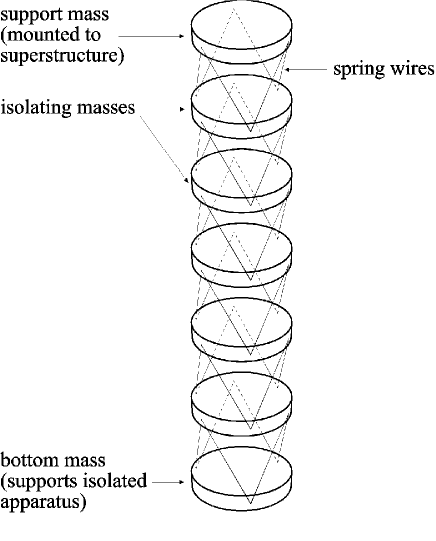
FIG. 1.: Basic geometry of six-stage Taber vibration isolator.

Sec. II presents an approximate analytical model of a TVI. The model yields simple formulae for the natural frequencies of an isolator with a single spring–mass pair (or “stage”), and an accurate solution for the normal modes of a complete isolation stack. Sec. III presents a numerical analysis of the normal modes of a multi–stage isolator and shows that the results agree very well with the analytical model. Sec. IV uses the single–stage natural frequency formulae to optimize the design of a multi–stage isolator for uniform attenuation in all degrees of freedom, given the specific geometrical constraint of finite stack length. The subsequent predictions for the number of stages and for the spring wire diameter are used to construct an actual TVI, which is described in Sec. V. The measurements of the natural frequencies of a single stage are compared with calculations from the analytical model and the numerical analysis.

II Approximate Analytical Model

The analytical model of the TVI is based on a combination of the lumped–element one–dimensional spring–mass chain shown in Fig. 2, and the single stage in Fig. 3. This model is exact for translations along and rotations about the vertical axis, and, as shown below, it gives a good approximation of the transverse motions as well.

A single stage with one degree of freedom (DOF) is useful for understanding the attenuation of a multi-stage isolator. If the spring is displaced at the top by a vibration of frequency $\omega$ (the frequency to be filtered by the isolator, or operating frequency) and amplitude $x(\omega)$, the equation of motion for this system may be written:

$$-m\omega^{2}x_{0}(\omega)=k[x(\omega)-x_{0}(\omega)],$$ (1)

where $m$ is the mass, $k$ is the spring constant, and $x_{0}(\omega)$ is the amplitude of the suspended mass. Re-arranging this equation yields the single–stage transfer function for one DOF:

$$T_{0}(\omega)\equiv\frac{x_{0}(\omega)}{x(\omega)}=\frac{\omega_{0}^{2}}{\omega_{0}^{2}-\omega^{2}},$$ (2)

where $\omega_{0}=\sqrt{k/m}$ is the natural frequency of the single–stage isolator.

The rest of this analysis considers operation frequencies well above the resonant frequencies of the system ($\omega\gg\omega_{0}$). In this regime, $T_{0}(\omega)=(\omega_{0}/\omega)^{2}$. In the case of an isolator of $n$ identical stages, each with natural frequency $\omega_{0}$ (Fig. 2), $x_{\mu}(\omega)\gg x_{\mu+1}(\omega)$ for the $\mu$th stage, so that Eq. 1 may be applied to each successive stage. The displacement of each stage with respect to that immediately above is then simply another factor of $(\omega_{0}/\omega)^{2}$, so that the attenuation in displacement from the support to the $n$th suspended mass, for one DOF, is given by $(\omega_{0}/\omega)^{2n}$. The extremely rapid dependence of the attenuation on frequency is, of course, the reason why multi-stage isolators are so effective.

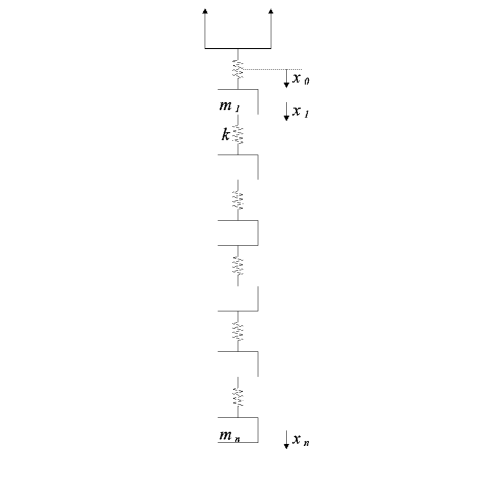
FIG. 2.: One–dimensional lumped–element spring–mass chain; basis of simple analytical model of Taber isolator.

The complete expression for the transfer function for an undamped system of $n$ stages with masses $m_{\mu}$, spring constants $k_{\mu}$, and one DOF is given by:[6]

$$T_{n}(\omega)\equiv\frac{x_{n}(\omega)}{x(\omega)}=\prod_{\mu=\nu=1}^{n}{\frac{k_{\mu}/m_{\mu}}{\Omega_{\nu}^{2}-\omega^{2}}}.$$ (3)

Here, $\sqrt{k_{\mu}/m_{\mu}}=\omega_{\mu}$ is the natural frequency of the $\mu$th stage, and $\Omega_{\nu}$ is the frequency of the $\nu$th normal mode. In the high frequency regime, this result reduces to $(\omega_{0}/\omega)^{2n}$, for an isolator with identical stages ($\omega_{\mu}=\omega_{0}$).

In order to use Eq. 3 to estimate the total attenuation of the TVI for each DOF, the analytical model can be used to approximate the single–stage frequencies $\omega_{\mu}$ and to calculate the normal mode frequencies $\Omega_{\nu}$. The first step is to derive the linear and torsional spring constants for each DOF.

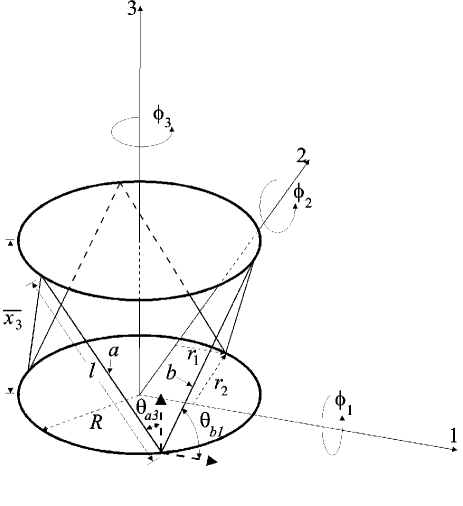
FIG. 3.: Single TVI stage with parameters used for calculation of spring constants.

A Spring Constants

Using the axes defined in Fig. 3, the normal modes of the TVI are modeled as pure translations along and rotations about the 1-, 2-, and 3-axes. This is an approximation because in reality the 1- and 2- translations and rotations are coupled. The evaluation of the spring constant for translation along the 3-axis is the most straightforward. In Fig. 3, $\theta_{a3}$ is the angle between the 3-axis and wire $a$, $\overline{x_{3}}$ is the equilibrium spacing between any two stages, $l$ is the length of the wire, $A$ is the cross-sectional area of the wire, and $E$ is the modulus of elasticity of the wire. In this analysis, each of these parameters is assumed to have a unique value for a particular stage. Since the basic geometry of all stages is the same, however, the functional form of the spring constants for each stage is also the same. The stage subscript, $\mu$, can therefore be dropped to economize the notation. The relationship between an infinitesimal force $dF$ along a spring wire and displacement $dl$ is then:

$$dF=-E\frac{A}{l}dl.$$ (4)

For an initial longitudinal displacement $dx_{3}$, the displacement along the wire is:

$$dl=dx_{3}\cos{\theta_{a3}}$$ (5)

so that:

$$dF=-E\frac{A}{l}\cos{\theta_{a3}}dx_{3}.$$ (6)

The longitudinal component of the force is then:

$$dF_{3}=-E\frac{A}{l}\cos^{2}{\theta_{a3}}dx_{3}.$$ (7)

This expression is equivalent for all six wires per stage, so that the total spring constant for motion along the 3-axis is:

$$k_{x_{3}}=6E\frac{A}{l}\cos^{2}{\theta_{a3}}=\frac{6EA(l^{2}-R^{2})}{l^{3}},$$ (8)

where $R$ is the radius of the stage, and we have used $R^{2}=l^{2}-x_{3}^{2}$ from the hexagonal geometry of the attachment points. In general, if $\theta$ is the angle between a wire and the direction of translation, the corresponding contribution to the spring constant for that DOF is $k=EA\cos^{2}{\theta}/l$.

Referring again to Fig. 3, two wires per stage have angle $(\pi/2)-\theta_{a3}$ with respect to the 1-axis. Their contribution to the corresponding spring constant is therefore $k=2EAR^{2}/l^{3}$. The remaining four wires each have angle $\theta_{b1}$ with respect to this axis, bringing the total spring constant to $k_{x_{1}}=3EAR^{2}/l^{3}$.

Finally, from the figure, four wires per stage have angle $\theta_{b2}$ with respect to the $2$-axis, so that their total contribution to the spring constant is $k=3EAR^{2}/l^{3}$. This is the complete expression for $k_{x_{2}}$, since the remaining two wires are orthogonal to the $2$-axis. These results are summarized in Table I.

Computation of the torsional spring constants is simplified by expressing the infinitesimal torques $d\tau_{j}$ about each axis in terms of the infinitesimal displacements $dx_{j}$ of the attachment points. If $d\phi_{j}$ is the infinitesimal rotation of the effective lever arm $r_{k}$ about the $j$th axis, we have, for each wire on the stage:

$$d\tau_{1}=r_{2}dF_{3}=-k_{\tau_{1}}d\phi_{1},$$ (9)

$$d\tau_{2}=r_{1}dF_{3}=-k_{\tau_{2}}d\phi_{2}.$$ (10)

Substituting $dF_{3}=-(k_{x_{3}}/6)dx_{3}$, $d\phi_{1}=dx_{3}/r_{2}$, and $d\phi_{2}=dx_{3}/r_{1}$ yields:

$$k_{\tau_{1}}=r_{2}^{2}\frac{k_{x_{3}}}{6},\ k_{\tau_{2}}=r_{1}^{2}\frac{k_{x_{3}}}{6}.$$ (11)

From the geometry in Fig. 3, only four wires contribute to the rotation of the stage about the 1-axis, each attached at a distance $r_{2}=R\sqrt{3}/2$ from that axis. The total torsional constant is therefore:

$$k_{\tau_{1}}=4\left(\frac{R\sqrt{3}}{2}\right)^{2}\frac{k_{x_{3}}}{6}=3EA\frac{R^{2}(l^{2}-R^{2})}{l^{3}}.$$ (12)

All six wires contribute to the rotation about the 2-axis, with two attached at a distance $r_{1}=R$ from the axis and the remaining four at $r_{1}=R/2$:

$$k_{\tau_{2}}=2R^{2}\frac{k_{x_{3}}}{6}+4\left(\frac{R}{2}\right)^{2}\frac{k_{x_{3}}}{6}=3EA\frac{R^{2}(l^{2}-R^{2})}{l^{3}}.$$ (13)

For the remaining torque about the 3-axis, we consider the force due to one wire at the attachment point lying on the 1-axis. Here, the force is along the 2-axis, so that

$$d\tau_{3}=r_{3}dF_{2}=-k_{\tau_{3}}d\phi_{3}.$$ (14)

Substituting $dF_{2}=-(k_{x_{2}}/4)dx_{2}$, $d\phi_{3}=dx_{2}/r_{3}$ yields:

$$k_{\tau_{3}}=r_{3}^{2}\frac{k_{x_{2}}}{4}.$$ (15)

From the symmetry of the stage about the 3-axis, the contribution of all six wires, each at a distance $r_{3}=R$ from the axis, must be the same. The total torsional constant is therefore:

$$k_{\tau_{3}}=6R^{2}\frac{k_{x_{2}}}{4}=\frac{9}{2}EA\frac{R^{4}}{l^{3}}$$ (16)

These results are included in Table I.

TABLE I.: Single-stage spring constants and natural frequencies for each DOF in the analytical model.

Motion	Spring Constant	Natural Frequency
Translation, 1- and 2-axes	$k_{x_{1}}=k_{x_{2}}=3EAR^{2}/l^{3}$	$w_{x_{1}}=w_{x_{2}}=R\sqrt{\frac{3EA}{ml^{3}}}$
Translation, 3-axis	$k_{x_{3}}=6EA(l^{2}-R^{2})/l^{3}$	$w_{x_{3}}=\sqrt{\frac{6EA(l^{2}-R^{2})}{ml^{3}}}$
Rotation, 1- and 2-axes	$k_{\tau_{1}}=k_{\tau_{2}}=3EAR^{2}(l^{2}-R^{2})/l^{3}$	$w_{\tau_{1}}=w_{\tau_{2}}=2\sqrt{\frac{3EA(l^{2}-R^{2})}{ml^{3}(1+\frac{1}{3}(\frac{t}{R})^{2})}}$
Rotation, 3-axis	$k_{\tau_{3}}=9EAR^{4}/(2l^{3})$	$w_{\tau_{3}}=3R\sqrt{\frac{EA}{ml^{3}}}$

B Resonant Frequencies

The natural frequencies for the translational modes of a particular stage are simply $\omega_{x_{j}}=\sqrt{k_{x_{j}}/m}$, where $j=1-3$ refers to each axis and $m$ is the mass of the disk. For the rotational modes, the natural frequencies are $\omega_{\tau_{j}}=\sqrt{k_{\tau_{j}}/I_{\tau_{j}}}$. Here, $I_{\tau_{3}}=mR^{2}/2$ is the moment of inertia of the disk about the 3-axis, and $I_{\tau_{1}}=I_{\tau_{2}}=mR^{2}(1+(t/R)^{2}/3)/4$ is the moment about the 1- and 2-axes, where $t$ is the disk thickness. The natural frequencies for each DOF are included in Table I.

For each DOF, the normal mode frequencies $\Omega_{\nu}$ must be calculated in a complete solution to the one–dimensional lumped–element spring–mass chain in Fig. 2. The choice of six stages for the model, while technically arbitrary at this point, is motivated by the results of the design optimization in Sec. IV. The analytical solution leads to a twelfth–order polynomial in $\omega$ for translation or rotation in the relevant coordinate. The normal mode frequencies $\Omega_{\nu}$ are computed by substituting the expressions for the spring constants in Table I into the characteristic equation and finding the roots numerically. The parameters entering into the characteristic equation (mass radii and thickness, wire length, diameter, and elastic modulus) also derive from the results of the optimization procedure in Sec. IV, and are listed in Tables II and III. The frequencies are plotted in Figs. 4 and  5. The twelve translational frequencies and twelve rotational frequencies for the 1- and 2-axes are two–fold degenerate.

Fig. 6 shows the transfer function evaluated for the case of six stages and $\omega_{\mu}=\omega_{0}$ for each stage. The highest normal mode frequency is close to $2\omega_{0}$ (this would be exact for an infinite chain), and the asymptotic attenuation is nearly reached at $\omega\approx 3\omega_{0}$.

The single–stage natural frequency $\omega_{0}$ nearly completely characterizes the behavior of a multi-stage TVI with identical stages. This frequency depends on the design parameters of the TVI in a simple and explicit way, and therefore can be used directly for design optimization. Before discussing optimization, the analytical model is compared to a numerical analysis.

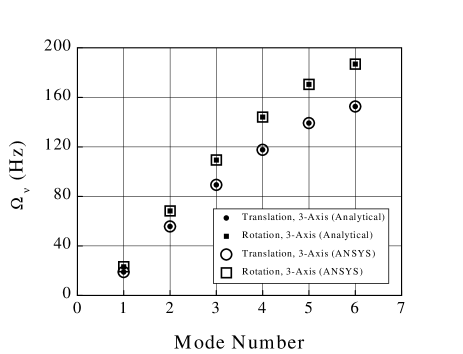
FIG. 4.: Resonant frequencies $\Omega_{\nu}$ vs. mode number for translations and rotations (3-axis).

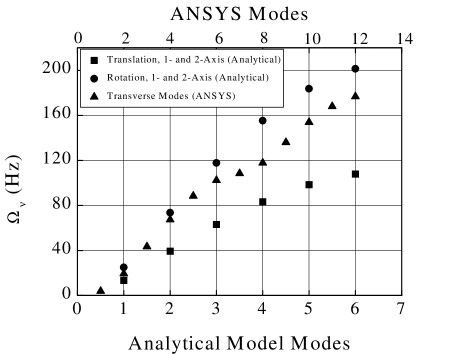
FIG. 5.: Resonant frequencies $\Omega_{\nu}$ for translations and rotations (1- and 2-axes). For the numerical analysis, frequencies are arranged by mode number (upper axis). For the analytical model, frequencies are arranged in increasing order for each DOF.

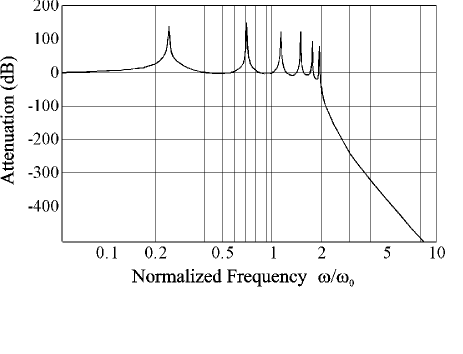
FIG. 6.: Transfer function vs. operation frequency for six–stage isolator.

III Finite Element Analysis

A numerical model of a six stage TVI is constructed using the ANSYS[9] finite element analysis software package. Rigid bodies with six DOF model the brass disks, and elastic beams, also with six DOF, model the steel wires. The beams are arranged in the geometry of the wires in Fig. 3, and are coupled rigidly at their endpoints to the point masses representing the disks. In addition to mass, the required input parameters for the point masses include the moments of inertia for each rotational DOF. The required input parameters for the beams include density and modulus of elasticity. All input parameters are derived from the data in Tables II and III.

The frequencies of the 36 normal modes calculated by ANSYS are compared to the frequency calculations from the analytical model in Figs. 4 and  5. The results in Fig. 4 show that the analytical model is exact for translations along and rotations about the 3-axis. In Fig. 5, remaining frequencies calculated in ANSYS are arranged by mode number (upper axis). The results from the analytical model are arranged by increasing frequency for each DOF. The plot illustrates that the true normal mode frequencies fall between the uncoupled translation and rotation frequencies found analytically.

This analysis suggests that the approximate analytical model of the TVI is sufficiently accurate for use in the development of a working design. Furthermore, for an isolator with identical stages operating in the high frequency domain, the single–stage resonant frequency $\omega_{0}$ for each DOF from the model is a sufficient parameter with which to optimize the design.

IV Design Optimization

From Eq. 3, the attenuation for a multi-stage isolator is most strongly dependent on the number of stages, $n$. While it is important to choose a sufficient number of stages for the degree of attenuation desired, the maximization of $n$ given the geometrical constraints of the system must be balanced with at least two other important factors. First, attention should be given to the extent to which attenuation is desired in each DOF of the isolated system. Second, it is essential that the transverse vibrational modes of the spring wires be kept well above the operational frequency, $\omega$, so that the wires function as simple springs.

A Uniform Isolation in each DOF

The particular application in our laboratory requires the isolation of vibrations in the kilohertz range in all DOF. The normal modes for each DOF of the TVI should therefore be essentially the same. Using the single–stage analytical model, relations between the geometrical parameters of the TVI can be found by equating the natural frequencies for each DOF.

From the expressions in Table I, the natural frequencies $\omega_{x_{1,2}}$ and $\omega_{\tau_{3}}$ always differ by a factor of $\sqrt{3}$. Taking an approximate average of these two terms and equating it to the other natural frequencies in the table yields:

$$\frac{6EAR^{2}}{ml^{3}}\approx\frac{6EA(l^{2}-R^{2})}{ml^{3}}\approx\frac{12EA(l^{2}-R^{2})}{ml^{3}(1+\frac{1}{3}(\frac{t}{R})^{2})}.$$ (17)

Simplifying:

$$R^{2}\approx(l^{2}-R^{2})\approx\frac{2(l^{2}-R^{2})}{(1+\frac{1}{3}(\frac{t}{R})^{2})}.$$ (18)

Equating the first two terms gives the relation $R=l/\sqrt{2}$. The second two terms yield $t=R\sqrt{3}$, and the remaining equality yields no new information. In terms of the wire length $l$, the disk radius and thickness are related by

$$R=l/\sqrt{2},\ t=l\sqrt{3/2}.$$ (19)

Ideally, Eq. 19 guarantees equal single–stage frequencies and therefore equal attenuation of vibrations for each DOF of the multi–stage TVI with identical stages. In practice this condition is relaxed somewhat, as explained in Sec. V and reflected in Figs. 4 and  5.

B Optimal Number of Stages

The maximum attenuation per DOF can now in principle be obtained by maximizing the number of stages $n$, subject to the above constraints. At this point, however, the design is of course limited by the geometrical constraints of the containment system and the properties of appropriate TVI construction materials.

With the equality of the natural frequencies of each DOF guaranteed by the constraints in the previous section, the attenuation may optimized based on motion in only one particular DOF. For the choice of longitudinal motion along the 3-axis, the single-stage transfer function is given by:

$$T_{0x_{3}}=\frac{\omega_{0}^{2}}{\omega^{2}}=\frac{1}{\omega^{2}}\frac{6EA(l^{2}-R^{2})}{ml^{3}}.$$ (20)

Expressing the disk mass $m$ in terms of the density $\rho_{d}$ and the dimensions of the disk yields:

$$T_{0x_{3}}=\frac{1}{\omega^{2}}\frac{6EA(l^{2}-R^{2})}{\pi\rho_{d}R^{2}tl^{3}},$$ (21)

and substituting Eq. 19 gives:

$$T_{0x_{3}}=\frac{1}{\omega^{2}}\frac{12EA}{\sqrt{3}\pi\rho_{d}l^{4}}.$$ (22)

The geometrical constraint of the containment system is modeled by limiting the total possible height of the stack to some finite value. This translates into a total finite length $L$ for all wires along one side of the stack. With $n$ total stages of equal length, the wire length $l$ per stage is $l=L/n$.

The cross-sectional area $A$ of the spring wires is limited by the elastic limit stress $s$, or the stress at which acoustic emission becomes intolerable. If $F$ is the force on one of the six wires supporting a single–stage isolator, the minimum cross-section is given by

$$A_{0}=\frac{F}{s}=\frac{\pi R^{2}t\rho_{d}g}{6s}.$$ (23)

As this point, the requirement that each stage in the multi-stage TVI model have equivalent geometry is relaxed in order to permit the minimum wire cross–section per stage. This results in a range of natural frequencies $\omega_{\mu}$ in the stack. However, as long as Eq. 19 is made to hold for each stage, and as long as $\omega_{\mu}\ll\omega$ for all $\mu$, the multi–stage TVI will still operate effectively in all DOF.

For the $\mu$th stage in a stack of $n$ stages (with $\mu=1$ corresponding to the top stage), the minimum wire cross section for that stage requires a factor of $(n-\mu+1)$ due to the weight of the stages below it. Substituting Eq. 19,

$$A_{\mu}=\frac{\pi l^{3}\rho_{d}g(n-\mu+1)}{4\sqrt{6}s}.$$ (24)

Ensuring the maximum tolerable force on each wire also has the effect of maximizing the frequencies of the transverse modes on the spring wires, an important point to be considered below.

Inserting the last expression into Eq. 22, and again using Eq. 19, the transfer function for the $\mu$th stage of the $n$-stage isolator is given by:

$$T_{\mu x_{3}}=\frac{\omega_{\mu}^{2}}{\omega^{2}}=\frac{n}{\omega^{2}}\frac{Eg(n-\mu+1)}{\sqrt{2}sL}.$$ (25)

The complete transfer function for the $n$-stage isolator is then the product of the factors for each stage:

$$T_{x_{3}} = \left(\frac{n}{\omega^{2}}\frac{Egn}{\sqrt{2}sL}\right)\left(\frac{n}{\omega^{2}}\frac{Eg(n-1)}{\sqrt{2}sL}\right)\left(\frac{n}{\omega^{2}}\frac{Eg(n-2)}{\sqrt{2}sL}\right)$$ (27)

$$\times\cdot\cdot\cdot\times\left(\frac{n}{\omega^{2}}\frac{Eg}{\sqrt{2}sL}\right)=\left(\frac{n}{\omega^{2}}\frac{Eg}{\sqrt{2}sL}\right)^{n}n!$$

This expression illustrates importance of using spring materials of low elastic modulus and high elastic limit. Fig. 7 shows a plot of $T_{x_{3}}$, using the parameters in Table II. The constraints specified in this model limit the exponential rise in attenuation with the number of stages ($T\approx(\omega_{1}/\omega)^{2n}$). At first glance, one might expect to attain a maximum attenuation of about 500 dB with 30 stages (1 dB $\equiv 20\log{T}$). However, this analysis applies only to the asymptotic regime, the upper limit of which, from Fig. 6, is defined by $\omega\simeq 3\omega_{0}$. From Eq. 25, the highest $\omega_{\mu}$ in the model corresponds to $\mu=1$:

$$w_{1}=\sqrt{\frac{n^{2}Eg}{\sqrt{2}sL}}.$$ (28)

Requiring $\omega_{1}<\omega/3$ in this expression yields $n<16$, suggesting that attenuations above 400 dB may still be possible.

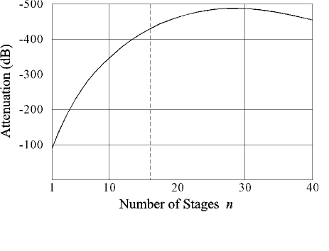
FIG. 7.: Attenuation ($T$) in dB vs. number of stages for analytical model of a TVI with operation frequency of 1 kHz and properties in Table II. The dashed line indicates the approximate limit of the asymptotic regime. Scale: 1 dB = 20 $\log{T}$.

C Effect of Spring Transverse Modes

In the design of a TVI, care must be taken to ensure that the frequencies of the transverse modes of the spring wires lie well above the operation frequency. Otherwise, the wires will not act as lumped–element springs.

The fundamental transverse frequency of a wire of length $l$ is given by:

$$\omega_{t}=\frac{\pi}{l}\sqrt{\frac{T}{\eta}},$$ (29)

where $T$ is the tension in the wire and $\eta$ is the wire mass per unit length. From the previous section, the tension in the wire is automatically maximized; it is just the elastic limit times the cross-section: $T=sA$. The mass per unit length is $\eta=\rho_{w}A$, where $\rho_{w}$ is the wire mass density. Applying Eq. 19, the lowest transverse frequency becomes:

$$\omega_{t}=\frac{n\pi}{L}\sqrt{\frac{s}{\rho_{w}}}.$$ (30)

This function is plotted in Fig. 8, using the parameters in Table II. For this model, any choice of $n$ greater than 3 insures that all transverse spring frequencies are at least twice the operational frequency.

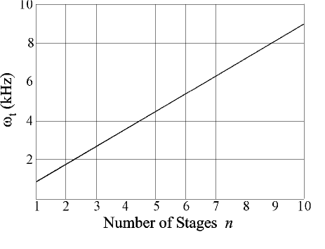
FIG. 8.: Frequency of spring wire fundamental transverse mode $\omega_{t}$ vs. number of stages for analytical model of a TVI with operation frequency of 1 kHz and properties in Table II.

An important assumption made in the optimization procedure is that the diameter of the spring wires is allowed to decrease on successively lower stages in the stack. From Eq. 24 for the cross-sectional area of the spring wires on a given stage, and using Eq. 19, the diameter of the spring wires on the $\mu$th stage of an $n$-stage TVI is given by:

$$d_{w}=\sqrt{\frac{L^{3}\rho_{d}g(n-\mu+1)}{\sqrt{6}n^{3}s}}.$$ (31)

The diameter is plotted as a function of stage number in Fig. 9, for the cases $\mu=1$ (top stage) and $\mu=n$ (bottom stage), using the parameters in Tables II and III. The values of the curves at a given $n$ define the range of wire diameters needed for the construction of a TVI with the attenuation shown in Fig. 7.

For $n>10$, the diameters required fall well below 25 $\mu$m, which may be a practical limit. Note the dependence of Eq. 31 on $\rho_{d}$, illustrating the importance of choosing stage masses of high density. Wires of larger diameter may be used at some cost of attenuation, but care should be taken to avoid transverse modes in the operating range.

V Construction and Test of Six–Stage Isolator

A Choice of Materials

The preceding discussion mandates a choice of a high–density material for the construction of the TVI masses. For our specific application, the masses must non-magnetic, and be vacuum and cryogenically compatible. An ideal choice would be tungsten, but brass is selected for its low cost and ease of machining.

The spring wires should have a combination of low elastic modulus and density, and, most importantly, high elastic limit. Beryllium copper and certain aluminum alloys have ideal characteristics, and have the added advantage of being non-magnetic. However, type 304 stainless steel is chosen for its availability at low cost in many different diameters.[10]

The construction of a TVI for a small laboratory application is considerably simplified if the spring wires can be made to attach to a set of coplanar screws bolted to the outer rim of each suspended disk, as suggested by Fig. 1. This makes impractical the requirement $t>l$, as derived in Sec. IV A. If the screws are set into the midplane of each disk, the hexagonal geometry of the attachment points guarantees the stage spacing to be $R$, as long as $R=l/\sqrt{2}$.

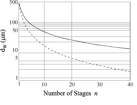
FIG. 9.: Wire diameter vs. number of stages for top stage (solid curve) and bottom stage (dashed curve) in analytical model of a TVI with operation frequency of 1 kHz and properties in Tables II and  III.

A simple choice would be to set both the stage thickness and the inter-stage gap to $R/2$. However, smaller disk thicknesses drive the frequencies of the 1- and 2-rotational modes higher relative to the other modes, so that $t\approx R/\sqrt{2}\approx l/2$ is a better choice. The rotational modes increase, but not enough to reach into the domain of the 1 kHz operating frequency (as seen in Fig. 5). In fact, this choice changes the optimization expressions used in Secs. IV B and IV C only by small numerical factors.

The size of our vacuum chamber limits the total height of the stack to 11.5 cm. With a stage separation distance $R$, the total wire length is then simply $L=R\sqrt{2}$, or 16.2 cm.

The total wire length needed and the properties of the mass and spring wire materials are listed in Tables II and  III. (These properties, and the operation frequency $\omega=$1 kHz, were used to generate the optimization curves in section  IV). To reduce the likelihood of acoustic emission, a value for the elastic limit of stainless steel equal to 1/3 the tabulated value is assumed.

TABLE II.: Properties of spring wires used in TVI model and construction.

Parameter	Value
Material	Type 304 Stainless Steel
Density, $\rho_{w}$	$8.05\times 10^{3}\mbox{\ kg/m}^{3}$
Elastic Modulus, $E$	$2.8\times 10^{11}\mbox{\ N/m}^{2}$
Elastic Limit a , $s$	$2.1\times 10^{9}\mbox{\ N/m}^{2}$
Total Length (along single row of posts), $L$	16.2 cm
Length per Stage, $l$	2.7 cm
Diameter, $d_{w}$	stage 1: $45\ \mu\mbox{m}$
	stages 2,3: $40\ \mu\mbox{m}$
	stages 4,5: $30\ \mu\mbox{m}$
	stage 6: $25\ \mu\mbox{m}$

TABLE III.: Properties of mass disks used in TVI model construction.

Parameter	Value
Material	Brass
Density, $\rho_{d}$	$8.5\times 10^{3}\mbox{\ kg/m}^{3}$
Radius, $R$	1.9 cm
Thickness, $t$	1.3 cm

The required degree of vibration isolation can be roughly estimated as the ratio of the force exerted by our gram–mass oscillator resonating at 1 kHz to the gravitational force between it and a similar oscillator spaced 1 mm away. This is roughly $10^{12}$, or 240 dB.

Reading off Fig. 7, 240 dB requires a stack of at least five stages. A six–stage design is chosen to conserve on labor and maintenance, which with fine wires can be delicate and time–consuming. Fig. 8 indicates that any transverse spring modes in a six–stage stack will have frequencies greater 5 kHz, safely above the operating range. Finally, Fig. 9 shows that a six–stage stack requires spring wire diameters ranging from about 30 to 80 $\mu$m.

The expected loss in attenuation due to the sub–optimal disk thickness can be compensated by choosing smaller wire gauges than specified in Fig. 9. The design is optimized assuming an elastic limit below the actual maximum, so the final design uses wire diameters ranging from 25 to 45 $\mu$m.

B Assembly

The choice of six stages fixes the length of each wire per stage to $l=L/n=16.2/6=2.7$ cm. The disks have dimensions $R=l/\sqrt{2}=1.9$ cm, $t=l/2=1.3$ cm, and are easily machined from brass stock. Seven disks are machined, with the first intended to attach to the support structure.

Holes are drilled and tapped into the center plane of each disk at 60 degree intervals to provide for the six 6-32 screws which serve as wire attachment posts. Additional holes are drilled into the top and bottom surfaces of the first and seventh disk, for mounting to the support structure and for attaching the isolated instruments.

Since the attachment of the wires is a delicate procedure, the seven disks must first be mounted securely. For this purpose, additional holes are drilled into the center plane of each disk, at 120 degree intervals. Three thin brass strips, each with seven holes spaced 1.9 cm apart, can then be attached to the stack using the extra holes, firmly fixing the disks in a vertical stack (Fig. 10).

With the strips in place, the wire attachment posts are assembled using the remaining holes in each disk. Each post consists of a vented aluminum spacer, a thin brass washer, and a thin nylon washer, secured to the disk with a vented screw (Fig. 11 and Table IV).

The posts are designed so that a single strand of spring wire can be used to support each stage, rather than six separate strands of wire. For example, in Fig. 10, one end of a 16.2 cm piece of wire is attached between the brass and aluminum washers at point A, and the other end is attached to a small weight. The wire is then woven between the washers at points B through F successively, and re-attached at point A. During this operation, as soon as the wire is woven around a particular post, the weighted end is left to hang while the post screw is tightened, thereby insuring uniform wire tension between each post. The nylon washer on each post is lubricated with vacuum pump oil, so that it does not rotate the brass washer (and thereby apply torque to the wire) as the screw is tightened.

As per the optimization procedure, wires of smaller gauges are used to connect successively lower stages, as specified in Table II. After all post screws are tightened on each stage, the brass strips are removed and the finished isolator is ready for use (Fig. 12).

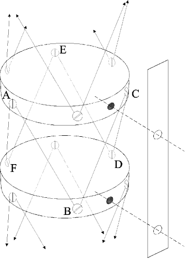
FIG. 10.: Wiring procedure for construction of multi–stage TVI (not to scale), showing a segment of one of the three temporary brass holding strips.

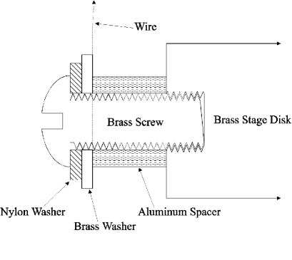
FIG. 11.: Cross–section of wire post construction on edge of stage disk (not to scale).

TABLE IV.: Items used in spring wire post construction.

Item	Material	Dimensions (mm)
6-32 Screw	Brass	9.5
Spacer	Aluminum	3.2 $\times$ 3.7 I.D. $\times$ 6.3 O.D.
Clamp Washer	Brass	0.8 $\times$ 3.7 I.D. $\times$ 9.5 O.D.
Guide Washer	Nylon	0.8 $\times$ 3.7 I.D. $\times$ 7.9 O.D.

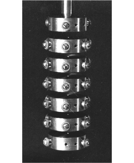
FIG. 12.: Photo of completed TVI.

C Single–Stage Test

The experimental verification of a multi–stage TVI is a challenging problem due to the difficulty of observing the multiple, closely–spaced normal modes and the highly attenuated motion of the lower stages. We limit ourselves here to checking the natural frequencies of a single stage.

The single–stage isolator is constructed using the materials and specifications in Tables II–IV (the diameter of the single wire is 30 $\mu$m). Using the same set of design parameters, plus some small refinements to include the wire posts, a finite element analysis is performed with ANSYS. The normal mode frequencies are also calculated analytically using formulae similar to those in Table  I, but with corrections for the effect of attaching the spring wires at points outside the disk radii, and for the additional rotational inertia due to the wire posts. These results are summarized in Table V.

TABLE V.: Natural frequencies for each DOF of a single–stage TVI.

	Analytical	ANSYS	Measurement
Motion	Model (Hz)	Result (Hz)	(Hz)
Translation, 1-axis	56	42	38
Translation, 2-axis	56	42	38
Translation, 3-axis	57	62	65
Rotation, 1-axis	86	96	98
Rotation, 2-axis	86	96	98
Rotation, 3-axis	110	101	102

As in the multi–stage case in Sec. III, the methods are in better agreement (within 9%) for translations along and rotations about the 3-axis. The 10–30% discrepancies between the other modes arise because the pure 1- and 2- translations and rotations assumed by the analytical model are only approximations of the actual motion for these modes. The ANSYS graphics indicate that these modes involve pendulum–type motions. The modes labeled “translations” in the transverse directions in Table V actually mix the translations with slight rotations about the transverse axes. Similarly, “rotations” mix with slight translations, so that the labels in Table V are to some extent misnomers for the case of the numerical analysis (and for the measurements).

The resonant frequencies of the single–stage TVI are measured with a PZT transducer. The transducer is bolted to the stage using one of the spare holes for the brass assembly strips, and the output is fed to a spectrum analyzer. Six frequencies are observed. In order to identify an observed frequency with a particular mode, the spectrum analyzer response is monitored as the sensitive axis of the PZT is oriented in each direction associated with the predominant motion of the predicted modes. The largest signal on the analyzer for a particular orientation is then recorded as the frequency of the associated mode.

Using this procedure, the six frequencies can be identified with expected modes. The measurements are plotted in Fig. 13, against the predictions from the finite element analysis. The results agree to within 10% for each frequency.

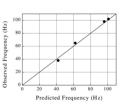
FIG. 13.: Measured resonant frequencies for single–stage isolator vs. numerical analysis predictions. The frequencies near 40 and 95 Hz are two–fold degenerate. Line indicates unit slope.

A conservative assumption is that the attenuation of the six–stage TVI at the operating frequency $\omega=1$ kHz is limited by the highest natural frequency. From Fig. 13, the highest frequency is $\omega_{0}\approx$ 100 Hz. The estimate of the attenuation is then $-20\log{(\omega_{0}/\omega)^{2n}}$ = 260 dB, in accordance with the model in Sec. V.

VI Conclusions

An approximate analytical model for a multi–stage TVI can be constructed from a one–dimensional spring–mass chain, in which the spring constants are derived from the geometry of a single stage. The full solution to this model makes exact predictions for the normal modes involving translations along and rotations about the longitudinal axis of the isolator, as computed with a finite element analysis. The model gives good approximations for the transverse modes as well.

The high–frequency behavior of an isolator with identical (or nearly identical) stages is well characterized by the natural frequencies of a single stage in all DOF, which are easily calculated with the model. These frequencies depend on the design parameters of the TVI in a straightforward way and are very useful for the design of a multi–stage isolator.

We have used the single–stage frequency formulae to design a fixed–length TVI for operation at 1 kHz in all DOF. The model illustrates the importance of selecting stage masses of high density, and spring materials of low elastic modulus and high elastic limit. The last quality is important for both the maximization of the attenuation and for ensuring that the transverse modes of the spring wires are well above the operating frequency.

The model makes accurate predicitons for the single–frequencies in the final design, which are in the range of 100 Hz. With six stages, the attenuation of our centimeter–scale TVI is estimated at 260 dB.

REFERENCES

- [1] W. M. Fairbank, M. Bassan, C. Chun, R. P. Giffard, J. N. Hollenhorst, E. Mapoles, M. S. McAshan, P. F. Michelson, and R. C. Taber, in Proceedings of the Second Marcel Grossmann Meeting on General Relativity, ed. R. Ruffini (Amsterdam, North-Holland, 1982).
- [2] P. F. Michelson, J. C. Price, and R. C. Taber, Science 237 150 (1987).
- [3] J. C. Long, H. W. Chan, and J. C. Price, Los Alamos Preprint hep-ph/9805217 (1998) (accepted for publication in Nuc. Phys. B, 16 Oct. 1998).
- [4] J. C. Price, in Proceedings of the International Symposium on Experimental Gravitational Physics, ed. P. Michelson, H. En-ke, and G. Pizzella (D. Reidel, Dordrecht, 1987).
- [5] R. N. Kleiman, G. Agnolet, and D. J. Bishop, Phys. Rev. Lett. 59 2079 (1987).
- [6] T. L. Aldcroft, P. F. Michelson, R. C. Taber, and F. A. McLoughlin, Rev. Sci. Instrum. 63 3815 (1992).
- [7] D. G. Blair, F. J. Van Kann, and A. L. Fairhall, Meas. Sci. Tech. 2 846 (1991).
- [8] J. Giaime, P. Saha, D. Shoemaker, and L. Sievers, Rev. Sci. Instrum. 67 208 (1996).
- [9] ANSYS/ED Release 5.3, SAS IP (1996), provided by ANSYS, Inc., 201 Johnson RD, Houston PA 15342-1300.
- [10] Wire purchased from California Fine Wire Co., Grover City CA 93433.