Classical evolution of quantum elliptic states

Abstract

The hydrogen atom in weak external fields is a very accurate model for the multiphoton excitation of ultrastable high angular momentum Rydberg states, a process which classical mechanics describes with astonishing precision. In this paper we show that the simplest treatment of the intramanifold dynamics of a hydrogenic electron in external fields is based on the elliptic states of the hydrogen atom, i.e., the coherent states of SO(4), which is the dynamical symmetry group of the Kepler problem. Moreover, we also show that classical perturbation theory yields the exact evolution in time of these quantum states, and so we explain the surprising match between purely classical perturbative calculations and experiments. Finally, as a first application, we propose a fast method for the excitation of circular states; these are ultrastable hydrogenic eigenstates which have maximum total angular momentum and also maximum projection of the angular momentum along a fixed direction.

32.80.Rm, 32.60.+i, 03.65.-w, 02.20.-a – Accepted for publication in Phys. Rev. A

I Introduction

In the past few years innovative experimental techniques have made possible the study of the dynamics of “Rydberg” electrons, that is, atomic electrons that are promoted to very high energy levels and that are only weakly bound to the atomic core [1]. The spectrum of such electrons is well described by a Rydberg-like formula (hence their name), and their wave functions are well approximated by eigenfunctions of the hydrogen atom with very large principal quantum number (typically $n\gtrsim 100$) [2]. Indeed, to a very good approximation the dynamics of Rydberg electrons is hydrogenic, and more complex atoms are often used in experiments merely as substitutes for hydrogen, because it is much easier to excite their valence electron to a Rydberg state, and yet the far-flung Rydberg electron senses a field which does not differ much from a pure Coulomb field. The recent experimental results have led to a renewed theoretical interest in the hydrogen atom in external fields in the limit of large quantum numbers, which is an exemplar for the study of quantum-classical correspondence in nonintegrable systems [3].

Indeed, recent experiments have shown that the intramanifold dynamics of large-n Rydberg electrons depends strongly on the presence of even surprisingly weak fields. This observation strongly suggests that it must be possible to manipulate accurately the quantum state of the electron by applying the appropriate combination of weak, slowly varying electric and magnetic fields. In fact, the theory of the hydrogen atom in weak fields is the basis of the treatment of slow ion-Rydberg collisions, which are generally considered to be the mechanism for the stabilization of the high-n states used in ZEKE (zero-electron-kinetic-energy) spectroscopy [4, 5, 6]. It also constitutes the starting point for the study of alkali atoms in weak, circularly polarized microwave fields [7, 8, 9, 10, 11].

An external electric field ${\mathbb{F}}$ is “weak” when its magnitude is small compared to the average Coulomb field sensed by the electron, that is, in atomic units (which we use throughout this paper)

$$F<<\frac{1}{n^{4}}\;.$$ (1)

In classical mechanics Eq. (1) implies that the energy of the Rydberg electron does not change significantly over a Kepler period, and classical perturbation theory applies. The condition on a magnetic field ${\mathbb{B}}$ is that the magnitude of the field must be much smaller than the Kepler frequency $\omega_{K}=1/n^{3}$ of the electron.

On the other hand, the quantum constraint on electric fields for negligible intermanifold mixing is the Inglis-Teller limit [2]

$$F<\frac{1}{3n^{5}}\;,$$ (2)

and for a very large n it may become a more stringent constraint than the classical one. The quantum constraint on a magnetic field $B$ is

$$B<\frac{1}{n^{4}}\;.$$ (3)

However, it has been recently shown that the more relaxed classical constraints hold also in quantum mechanics. That is, even in the presence of some intermanifold mixing the slow secular dynamics, due to the external fields, is essentially the same as if the Rydberg electron were still confined within a given n-manifold, because the time-averaged corrections due to n-mixing are negligible for large n [12]. Therefore in this paper we consider only the intramanifold dynamics of the Rydberg electron, and we assume that the external fields satisfy the Inglis-Teller limit, and also Eq. (3).

This paper is organized as follows: in Sec. II we discuss the evolution in time of atomic elliptic states in weak fields, and we show that they evolve exactly like the underlying classical ellipse; in Sec. III we propose an original approach to the production of circular Rydberg states, which is based on the dynamics of the coherent states of $SO(4)$; finally, in Sec. IV we draw some general conclusions.

II Perturbative dynamics in quantum and classical mechanics

The Hamiltonian for a hydrogen atom in crossed electric and magnetic fields reads

$$H=\frac{p^{2}}{2}-\frac{1}{r}+\frac{B}{2}L_{z}+Fx+\frac{B^{2}}{8}(x^{2}+y^{2})\;,$$ (4)

where the electric field is parallel to the $x$ axis and its strength is $F$; the magnetic field is parallel to the $z$ axis and its strength is $B$.

For weak fields the diamagnetic term, which is proportional to the square of the field, can be neglected. The simplified problem has been first solved quantum mechanically by Demkov et al. [13, 14]. However, their formal solution does not provide physical insight in the dynamics of the angular momentum of the Rydberg electron; it also becomes computationally intractable in the limit of large n’s.

The analysis of the intramanifold dynamics in the hydrogen atom rests on Pauli’s replacement, which is an operator identity between the position operator ${\bf{\hat{r}}}$ and the scaled Runge-Lenz vector operator ${\bf{\hat{a}}}$ (throughout this paper we use boldface letters for vectors, and we indicate a quantum operator with a caret), and which holds only within a hydrogenic n-manifold [15, 16]:

$${\bf{\hat{r}}}=-\frac{3}{2}n{\bf{\hat{a}}}\;.$$ (5)

The scaled Runge-Lenz vector operator ${\bf{\hat{a}}}$ is a hermitian operator, which for a bound state is defined as

$${\bf{\hat{a}}}=\frac{1}{\sqrt{-2E}}\left\{\frac{1}{2}\left({\bf{\hat{p}}}\times{\bf{\hat{L}}}-{\bf{\hat{L}}}\times{\bf{\hat{p}}}\right)-\frac{{\bf{\hat{r}}}}{r}\right\}\;,$$ (6)

where $E=-1/2n^{2}$ is the Kepler energy of the electron.

The angular momentum and the Runge-Lenz vector are invariants of the Kepler problem, and they commute with the hydrogenic Hamiltonian. By neglecting the diamagnetic term and using the identity of Eq. (5), in the interaction representation the perturbation Hamiltonian for external fields of arbitrary orientation becomes

$${\hat{H}}_{1}=-{\boldsymbol{\omega}}_{S}\cdot{\bf{\hat{a}}}-{\boldsymbol{\omega}}_{L}\cdot{\bf{\hat{L}}}\;,$$ (7)

where ${\boldsymbol{\omega}}_{S}=3n{\bf F}/2$ is the Stark frequency of the electric field, and ${\boldsymbol{\omega}}_{L}=-{\bf B}/2$ is the Larmor frequency of the magnetic field (we define the vector Larmor frequency with a minus sign, so that the dynamics is formally identical to the one of a negative charge in a noninertial rotating frame - see below).

The components of the angular momentum, plus those of the Runge-Lenz vector constitute the generators of $SO(4)$, which is the dynamical symmetry group of the Kepler problem [16]. It is convenient to decompose $SO(4)$ in the direct product of two rotation groups, i.e. $SO(4)=SO(3)\times SO(3)$, and we consider the following operators:

$$\begin{split}{\bf{\hat{J}}}_{1}&=\frac{1}{2}\left({\bf{\hat{L}}}+{\bf{\hat{a}}}\right)\\ {\bf{\hat{J}}}_{2}&=\frac{1}{2}\left({\bf{\hat{L}}}-{\bf{\hat{a}}}\right)\;.\end{split}$$ (8)

It is well known that ${\bf{\hat{J}}}_{1}$ and ${\bf{\hat{J}}}_{2}$ commute with each other and that their components constitute a realization of the angular momentum algebra [16]. The perturbation Hamiltonian can be rewritten as

$${\hat{H}}_{1}=-{\boldsymbol{\omega}}_{1}\cdot{\bf{\hat{J}}}_{1}-{\boldsymbol{\omega}}_{2}\cdot{\bf{\hat{J}}}_{2}\;,$$ (9)

where

$$\begin{split}{\boldsymbol{\omega}}_{1}&={\boldsymbol{\omega}}_{L}+{\boldsymbol{\omega}}_{S}\\ {\boldsymbol{\omega}}_{2}&={\boldsymbol{\omega}}_{L}-{\boldsymbol{\omega}}_{S}\;.\end{split}$$ (10)

Moreover ${\bf{\hat{L}}}$ and ${\bf{\hat{a}}}$ obey two constraints:

$$\begin{split}&{\bf{\hat{L}}}\cdot{\bf{\hat{a}}}=0\\ &{\bf{\hat{L}}}^{2}+{\bf{\hat{a}}}^{2}=n^{2}-1\;,\end{split}$$ (11)

and so one has

$$\begin{split}&{\bf{\hat{J}}}_{1}^{2}={\bf{\hat{J}}}_{2}^{2}=j(j+1)\\ &2j+1=n\;.\end{split}$$ (12)

Therefore both irreducible representations of $SO(3)$ have the same dimension, which is related to the principal quantum number n of the hydrogenic manifold.

Equation (9) reduces the problem to the dynamics of two uncoupled spins in the external “magnetic fields” ${\boldsymbol{\omega}}_{1}$ and ${\boldsymbol{\omega}}_{2}$. The analysis is particularly simple when the two “magnetic fields” ${\boldsymbol{\omega}}_{1}$ and ${\boldsymbol{\omega}}_{2}$ have constant orientation in space. However, all the considerations below also hold in the more general situation of arbitrary fields within the constraints of perturbation theory [17, 18], and we discuss explicitly the greater generality of our analysis later in this section. In the case of “magnetic fields” with constant orientation the propagator is simply

$${\hat{U}}(t^{\prime\prime},t^{\prime})=e^{i\int_{t^{\prime}}^{t^{\prime\prime}}{\boldsymbol{\omega}}_{1}\cdot{\bf{\hat{J}}}_{1}dt}e^{i\int_{t^{\prime}}^{t^{\prime\prime}}{\boldsymbol{\omega}}_{2}\cdot{\bf{\hat{J}}}_{2}dt}\;.$$ (13)

The elliptic eigenstates of the hydrogen atom [19, 20, 21, 22, 23] are nothing other than the coherent states of $SO(4)$ and therefore they can be expressed as the direct product of two coherent states of $SO(3)$. In turn, the coherent states of $SO(3)$ can be constructed quite generally by applying any operator of the group (i.e., any rotation) to the angular momentum eigenstate with maximum projection of the angular momentum along the z axis [17, 18]:

$$|j{\bf n}_{1},j{\bf n}_{2}\rangle=e^{i{\boldsymbol{\Omega}}_{1}\cdot{\bf{\hat{J}}}_{1}}e^{i{\boldsymbol{\Omega}}_{2}\cdot{\bf{\hat{J}}}_{2}}|jj_{1,z}=j\rangle\otimes|jj_{2,z}=j\rangle\;,$$ (14)

where ${\boldsymbol{\Omega}}_{1}$ and ${\boldsymbol{\Omega}}_{2}$ represent 3-dimensional active rotations, which respectively overlap the z axis with the unit vectors ${\bf n}_{1}$ and ${\bf n}_{2}$.

Clearly, angular momentum eigenstates that have maximum projection along the z axis are minimum uncertainty states for the angular momentum [17, 18], and the rotations of Eq. (14) preserve this property. The coherent states of $SO(3)$ are then states of minimum uncertainty for the angular momentum, and in their representation on the unit sphere they are sharply localized along the direction of the corresponding classical angular momentum. Similarly, elliptic states are localized along the directions of both classical “angular momenta” ${\bf J}_{1}$ and ${\bf J}_{2}$, i.e. along the unit vectors ${\bf n}_{1}$ and ${\bf n}_{2}$. It follows from Eq. (8) that they also possess well localized, quasiclassical angular momentum L and Runge-Lenz vector a.

FIG. 1.: Probability density (averaged along the z axis) of an atomic elliptic state localized on the xy plane. The principal quantum number is $n=30$, and the eccentricity is $e_{c}=0.6$. Both x and y vary between $-2n^{2}$ and $+2n^{2}$ (recall that in atomic units the Bohr radius is equal to one), and the nucleus is at the origin of the frame of reference. The probability density is sharply concentrated on the xy-plane, and we have averaged it over the z axis to show that the electron is more likely to be far from the nucleus. The peak at the aphelion which reflects the larger probability of finding the electron away from the nucleus is a purely classical effect. Because the classical electron is slower at the aphelion than at the perihelion it spends a longer time away from the nucleus than in its proximity, and the classical probability of finding a Rydberg electron far from the nucleus is larger. The figure was produced using the elegant formula for the wave function of atomic elliptic states derived in Ref. [20].

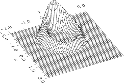
The classical objects that correspond to elliptic states are points in the phase space of the Kepler problem. In the more familiar configuration space these points are the trajectories of a classical electron in a pure Coulomb potential, i.e., Kepler ellipses, which are completely identified by the magnitude and direction of the two classical vectors ${\bf L}$ and ${\bf a}$ [24]. Indeed, the probability density of a hydrogenic electron in an elliptic state is peaked precisely along a Kepler ellipse (see Fig. 1).

Most importantly, it is easy to see that the propagator of Eq. (13) is also an operator of SO(4), and so when the propagator acts on an elliptic state it naturally yields some other elliptic state. More precisely, elliptic states are constructed by applying two rotation operators which map the z axis (that is, the direction of the angular momenta of the original states) onto some desired directions ${\bf n}_{1}$ and ${\bf n}_{2}$. Similarly, the propagator of Eq. (13) consists of two rotations respectively around the spatial axes given by the “magnetic fields” ${\boldsymbol{\omega}}_{1}$ and ${\boldsymbol{\omega}}_{2}$. The net effect of the propagator onto an elliptic state is:

$${\hat{U}}(t^{\prime\prime},t^{\prime})|j{\bf n}_{1},j{\bf n}_{2}\rangle=|j{\bf n^{\prime}}_{1},j{\bf n^{\prime}}_{2}\rangle\;,$$ (15)

where the two final unit vectors ${\bf n^{\prime}}_{1}$, ${\bf n^{\prime}}_{2}$ can be obtained from the initial ones by a clockwise classical precession around ${\boldsymbol{\omega}}_{1}$ and ${\boldsymbol{\omega}}_{2}$.

The original idea of studying the dynamics of elliptic states in weak fields is due to Nauenberg [23], who treated in detail the case of orthogonal, time-dependent electric and magnetic fields. In his analysis the connection with classical mechanics emerges for a configuration of the fields which constitutes a realization of $SO(3)$. We generalize his results to arbitrary fields, that is, to realizations of $SO(4)$, the full dynamical symmetry group of the Hydrogen atom. Indeed, most of the interest concerning elliptic states has been focused on the quasiclassical localization properties of the electron in real space [19, 20, 21, 22, 23], and the representation of elliptic states as a direct product of two coherent states of $SO(3)$ (which yields their time dependence so naturally and so generally) is not particularly suited for the study of the probability density of Rydberg electrons in real space.

In general, the classical object which corresponds to a coherent state is the classical phase space point which labels the state itself [17, 18]. A point in phase space is equivalent to a trajectory of the electron, which in the case of the Coulomb potential is a Kepler ellipse. Therefore the classical counterpart to the motion of the coherent states of $SO(4)$ is the dynamics of classical ellipses in weak fields, which is the object of study in classical perturbation theory, where the ellipse becomes the dynamical object itself [25, 26, 27, 5] .

In classical perturbation theory it is assumed that the electron still moves along an unperturbed ellipse, and the equations of motion describe how the elements (in the sense of celestial mechanics [28]) of the ellipse slowly vary in time. Clearly, an ellipse can be described by several equivalent sets of elements, however, if one chooses the angular momentum ${\bf L}$ and the Runge-Lenz vector ${\bf a}$ (the magnitude of the latter being proportional to the eccentricity of the ellipse) the equations of motion turn out to be particularly simple. More formally, in classical mechanics the angular momentum and the Runge-Lenz vector are constants of motion for the pure Kepler problem, i.e., their Poisson brackets with the Hamiltonian vanish, just like the commutators of the corresponding quantum operators. However, L and a become time-dependent as soon as applied external fields break the SO(4) symmetry of the Hamiltonian. In the case of very weak fields the effects of the perturbation take place on a time scale much longer than the Kepler period $T_{K}=2\pi n^{3}$. By simply averaging the equations of motion over a Kepler period and along an unperturbed Kepler ellipse one can easily derive the dynamics for the time-averaged angular momentum and the time-averaged Runge-Lenz vector, which for the sake of simplicity we still indicate with ${\bf L}$ and ${\bf a}$, and one has [25, 26, 27, 5]:

$$\begin{split}\frac{d{\bf L}}{dt}&=-{\boldsymbol{\omega}}_{S}\times{\bf a}-{\boldsymbol{\omega}}_{L}\times{\bf L}\\ \frac{d{\bf a}}{dt}&=-{\boldsymbol{\omega}}_{S}\times{\bf L}-{\boldsymbol{\omega}}_{L}\times{\bf a}\;.\end{split}$$ (16)

Like in quantum mechanics, the dynamics is particularly straightforward when it is expressed in terms of the “angular momenta” ${\bf J}_{1}$ and ${\bf J}_{2}$, which obey simple, uncoupled equations:

$$\begin{split}\frac{d{\bf J}_{1}}{dt}&=-{\boldsymbol{\omega}}_{1}\times{\bf J}_{1}\\ \frac{d{\bf J}_{2}}{dt}&=-{\boldsymbol{\omega}}_{2}\times{\bf J}_{2}\;,\end{split}$$ (17)

where the two frequencies are the same as in Eq. (10). The two classical spin vectors ${\bf J}_{1}$ and ${\bf J}_{2}$ simply precess clockwise around the “magnetic fields” ${\boldsymbol{\omega}}_{1}$ and ${\boldsymbol{\omega}}_{2}$, just like their quantum counterparts.

This shows that elliptic states in weak fields not only do evolve into elliptic states, and therefore retain their coherence properties and their localization along a classical Kepler ellipse, but they also evolve exactly according to the laws of classical mechanics (in the perturbative limit). This result has been already observed numerically and discussed theoretically for special fields configurations in Refs. [29, 30], and also in Ref. [23], where the case of orthogonal electric and magnetic fields is discussed. Most importantly, the same result has been observed also experimentally [7].

Indeed, we have illustrated explicitly the connection between quantum and classical mechanics only for a special configuration of the fields. However, our approach is based on the dynamics of the coherent states of $SO(4)$ and that guarantees -see below- that our conclusions hold for arbitrary fields (within the constraints of perturbation theory). Therefore, our study provides an analytical explanation of the numerical results and it also generalizes the previous theoretical arguments [29, 30, 23]. The main conclusions of our analysis do not depend on the particular choice of external fields; instead, they rest on the equivalence between the intramanifold dynamics of a Rydberg electron in weak external fields, and the motion of two uncoupled spins in external magnetic fields, and also on the properties of the coherent states of the angular momentum. It is well known that the coherent states of $SO(3)$ in arbitrary magnetic fields evolve in time exactly like the corresponding classical spin vectors [17, 18], and that is the reason why our demonstration holds for arbitrary electric and magnetic fields. Although the arguments for the classical evolution of quantum elliptic states hold in general, for fields with complicated time-dependence the explicit form of the propagator may be difficult to derive analytically. However, it is easy to see that it must be given by some combination of rotation operators. It is easy to see that in general the Euler angles of the propagator for a spin in a magnetic field obey some complicated, nonlinear differential equations that must be solved numerically, when the time dependence of the field is not trivial [17, 18]. However, when a numerical treatment is necessary, it is clearly much simpler to solve the classical, linear Eqs. (17). In fact, the classical equations yield directly the unit vectors ${\mathbb{n}^{\prime}}_{1}$ and ${\mathbb{n}^{\prime}}_{2}$, which label and determine completely the coherent state after it has evolved in time.

The quantum propagator of Eq. (13) is just the solution for a very special configuration of the external fields, however it is very useful because of its illustrative character, and of its relevance to ion-Rydberg collisions, which have been investigated experimentally. Moreover, for such fields the classical dynamics of the unit vectors labeling the elliptic state becomes amenable to an exact analytical treatment and it yields a most intuitive understanding of the dynamics, and we exploit this final characteristic in the next section.

A slowly rotating electric field is equivalent to crossed electric and magnetic fields in the noninertial frame rotating with the field [24, 14, 5]. Therefore our analysis explains why calculations based on purely classical methods account so well for several experimental results, ranging from slow ion-Rydberg collisions [4, 5, 6] to the dynamics of circular states in circularly polarized fields [7, 9], and to the anomalous scaling of the autoionization lifetimes of alkaline-earth Rydberg atoms also in circularly polarized microwave fields [8, 10]. Indeed, a classical trajectory Monte Carlo simulation based on Eqs. (17) is almost equivalent to a quantum treatment, in which the initial state is represented as a superposition of coherent states of $SO(4)$. That is, an elliptic state which is localized along a classical ellipse follows that same ellipse during its time evolution. Clearly, the quantum state is always somewhat diffuse, which is not true for a classical orbit. On the other hand, the overlap between two elliptic states with different angular momentum and Runge-Lenz vector is [17, 18]:

$$\left|\langle j{\bf n}_{1},j{\bf n}_{2}|j{\bf n^{\prime}}_{1},j{\bf n^{\prime}}_{2}\rangle\right|^{2}\\ =\left(\frac{1+{\bf n}_{1}\cdot{\bf n^{\prime}}_{1}}{2}\right)^{n-1}\left(\frac{1+{\bf n}_{2}\cdot{\bf n^{\prime}}_{2}}{2}\right)^{n-1}\;,$$ (18)

and because ${\bf n}_{i}\cdot{\bf n^{\prime}}_{i}\leq 1$ in the limit of large quantum numbers elliptic states behave more and more like sharply localized classical ellipses.

The time evolution of the classical vectors ${\bf J}_{1}$ and ${\bf J}_{2}$ which describe a Kepler ellipse can be expressed in terms of a classical propagator, that is

$${\bf J}_{i}(t^{\prime\prime})=U^{\rm cl}_{i}(t^{\prime\prime},t^{\prime}){\bf J}_{i}(t^{\prime})\;\;\;\;i=1,2\;,$$ (19)

and we conclude this section by writing explicitly the classical propagator for the important case when ${\boldsymbol{\omega}}_{1}$ and ${\boldsymbol{\omega}}_{2}$ have constant orientation in space, that is

$${\boldsymbol{\omega}}_{i}=\omega_{i}(t){\bf n}_{\omega_{i}}\;,\;{\bf n}_{\omega_{i}}=\left({\tilde{\omega}}_{ix},{\tilde{\omega}}_{iy},{\tilde{\omega}}_{iz}\right)\;\;\;\;i=1,2\;,$$ (20)

where ${\tilde{\omega}}_{ix}$, ${\tilde{\omega}}_{iy}$ and ${\tilde{\omega}}_{iz}$ are the components of the unit vector ${\bf n}_{\omega_{i}}$ that points along ${\boldsymbol{\omega}}_{i}$. First we set

$$\phi_{i}=\int_{t^{\prime}}^{t^{\prime\prime}}dt\omega_{i}(t)\;\;\;\;i=1,2\;,$$ (21)

and the classical propagator is

$$U^{\rm cl}_{i}(t^{\prime\prime},t^{\prime})=\cos\phi_{i}\cdot I-\sin\phi_{i}\cdot N_{i}\\ +(1-\cos\phi_{i})P_{i}\;\;\;\;i=1,2\;,$$ (22)

where $I$ is the identity matrix and the matrices $N_{i}$ and $P_{i}$ are respectively defined as follows:

$$N_{i}=\begin{pmatrix}0&-{\tilde{\omega}}_{iz}&{\tilde{\omega}}_{iy}\\ {\tilde{\omega}}_{iz}&0&-{\tilde{\omega}}_{ix}\\ -{\tilde{\omega}}_{iy}&{\tilde{\omega}}_{ix}&0\end{pmatrix}\;\;\;\;i=1,2\;,$$ (23)

and

$$P_{i}=\begin{pmatrix}{\tilde{\omega}}_{ix}^{2}&{\tilde{\omega}}_{ix}{\tilde{\omega}}_{iy}&{\tilde{\omega}}_{ix}{\tilde{\omega}}_{iz}\\ {\tilde{\omega}}_{iy}{\tilde{\omega}}_{ix}&{\tilde{\omega}}_{iy}^{2}&{\tilde{\omega}}_{iy}{\tilde{\omega}}_{iz}\\ {\tilde{\omega}}_{iz}{\tilde{\omega}}_{ix}&{\tilde{\omega}}_{iz}{\tilde{\omega}}_{iy}&{\tilde{\omega}}_{iz}^{2}\end{pmatrix}\;\;\;\;i=1,2\;.$$ (24)

As we argued before, the very same classical propagator also maps the unit vectors ${\bf n}_{1}$ and ${\bf n}_{2}$, which identify an elliptic state, precisely into the new unit vectors ${\bf n^{\prime}}_{1}$ and ${\bf n^{\prime}}_{2}$ of Eq. (15), i.e. the unit vectors which label the elliptic state after it has evolved in time according to the quantum-mechanical propagator.

However, when ${\boldsymbol{\omega}}_{1}$ and ${\boldsymbol{\omega}}_{2}$ have constant orientation the dynamics can be understood more intuitively by a geometric interpretation, as we illustrate more clearly in the next section.

III excitation of circular states

As a first application, in this section we describe an alternative method for the excitation of circular states, that is, hydrogenic states of maximum angular momentum.

Several diverse techniques have already been proposed and successfully implemented for the excitation of circular states and more generally of large-L elliptic states [31, 32, 33, 34, 35]. However, all these methods are based on the adiabatic manipulation of the Rydberg electron wave function. First, the electron is excited to an eigenstate of the Hamiltonian of the hydrogen atom in weak fields, and next the external fields are slowly varied in time while the electron always remains adiabatically in the same eigenstate of the Hamiltonian. Therefore in all such techniques the time scale that defines the adiabatic regime is determined by the inverse of the spacing of the energy levels of the hydrogen atom in weak fields. In practice, this means that a transformation is “adiabatic” if it takes place during a time much longer than the Stark or Larmor period of the Rydberg electron.

However, ground state electrons are typically excited to high-n Rydberg states via a few optical transitions, and initially they are confined to low angular momentum states. This causes some problems, because low-l Rydberg electrons are strongly coupled to the atomic (or molecular) core, which enhances the probability of decaying out of the Rydberg state. To the end of stabilizing the Rydberg electron it is then useful to increase the angular momentum of the state as quickly as possible [36]. We propose a technique which is adiabatic with respect of the Kepler period of the electron, which is a much shorter time than the Stark or Larmor periods (by a factor $\sim 1/n$). In fact, we do not try to maintain the electron in an eigenstate of the Hamiltonian at all times, and we only require that the dynamics must be confined within a hydrogenic n-manifold.

Our approach is based on the dynamics of elliptic states in weak external fields (a method based on the same dynamics was suggested in Refs. [29, 23]), and because we have shown that the evolution of these states is purely classical, we can discuss the excitation of circular states using classical mechanics. For a hydrogen atom in an electric field the red and blue Stark states with $m=0$ ($m$ being the usual magnetic quantum number) are two limit cases of elliptic states [19, 20, 21, 22, 23]. They correspond to two classical ellipses with maximum eccentricity, which have collapsed to a straight line. Individual high-n Stark states can be accessed directly from low energy states via an optical transition, and we assume that the Rydberg electron is initially placed in the blue Stark state, with $m=0$ (the same derivation applies also to electrons initially in the red Stark state). The fields configuration under which the Stark state evolves into a circular state could be derived analyzing the classical propagator of Eq. (22), however we present a more intuitive interpretation of the dynamics, which is based on a geometrical description of the time evolution.

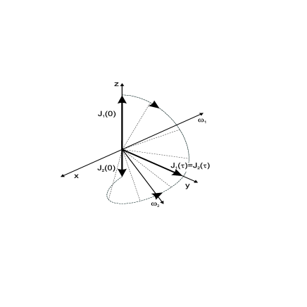
The external Stark field points along the positive z axis, and so does the Runge-Lenz vector of the blue Stark state, which means that the two angular momenta ${\bf J}_{1}$ and ${\bf J}_{2}$ point respectively along the $+z$ and $-z$ axis (see Fig. 2). Clearly, the angular momentum ${\bf L}$ of the state vanishes, as it must for an extreme Stark state. Our goal is to maximize ${\bf L}$, and therefore we need a configuration of external fields which will align ${\bf J}_{1}$ and ${\bf J}_{2}$ so to maximize their sum (${\bf L}={\bf J}_{1}+{\bf J}_{2}$) and minimize their difference (${\bf a}={\bf J}_{1}-{\bf J}_{2}$). We construct such fields by rotating the Stark field counterclockwise (recall that a rotating electric field is equivalent to crossed electric and magnetic fields [24, 14, 5]) around the y axis, and we also vary in time both the magnitude of the field and its rotation frequency, that is:

$${\bf F}(t)=F(t)\left[\cos\left(\int_{0}^{t}\omega_{R}(t^{\prime})dt^{\prime}\right){\bf n}_{z}\right.\\ +\left.\sin\left(\int_{0}^{t}\omega_{R}(t^{\prime})dt^{\prime}\right){\bf n}_{x}\right]\;,$$ (25)

where ${\bf n}_{z}$ and ${\bf n}_{x}$ are respectively unit vectors along the z and x axis, and $\omega_{R}(t)$ is the time dependent rotation frequency. We also set some final time $\tau$, which must be long compared to the Kepler period to insure that the motion is confined within an n-manifold. We require that at such time $\tau$ the field vanishes, so that the evolution of the elliptic state halts exactly when it becomes a circular state, that is,

$$F(\tau)=0\;.$$ (26)

In other words, as we slowly rotate the Stark field we also slowly turn it off.

The effect of the field of Eq. (25) is best analyzed in a frame rotating with the field. A rotating frame is not a Galilean frame, and the inertial effects of the Coriolis forces can be described exactly by introducing an effective Larmor frequency equal to the rotation frequency ${\boldsymbol{\omega}}_{R}$ of the frame of reference [24, 14, 5]. Therefore the equations of motion in the rotating frame are

$$\begin{split}\frac{d{\bf J}_{1}}{dt}&=-\left({\boldsymbol{\omega}}_{R}+{\boldsymbol{\omega}}_{S}\right)\times{\bf J}_{1}\\ \frac{d{\bf J}_{2}}{dt}&=-\left({\boldsymbol{\omega}}_{R}-{\boldsymbol{\omega}}_{S}\right)\times{\bf J}_{2}\;,\end{split}$$ (27)

where ${\boldsymbol{\omega}}_{R}$ and ${\boldsymbol{\omega}}_{S}$ point respectively along the y and z axis. We then require that at all times

$$\omega_{R}(t)=\omega_{S}(t)\;,$$ (28)

so that the axes of precession for ${\bf J}_{1}$ and ${\bf J}_{2}$ have constant orientation in space. The axes of precession have constant orientation in space also when the two frequencies are simply proportional to each other, but the analysis of the dynamics is much simpler when the Stark and rotation frequencies are exactly equal.

As we argued before, the two spin vectors precess around the two following “magnetic fields”:

$$\begin{split}{\boldsymbol{\omega}}_{1}&={\boldsymbol{\omega}}_{R}+{\boldsymbol{\omega}}_{S}\\ {\boldsymbol{\omega}}_{2}&={\boldsymbol{\omega}}_{R}-{\boldsymbol{\omega}}_{S}\;,\end{split}$$ (29)

where ${\boldsymbol{\omega}}_{1}$ and ${\boldsymbol{\omega}}_{2}$ lie in the yz plane, and ${\boldsymbol{\omega}}_{1}$ bisects the angle between the $+y$ and $+z$ axes, whereas ${\boldsymbol{\omega}}_{2}$ bisects the angle between the $+y$ and $-z$ axes.

It is easy to see from Fig. 2 that a clockwise precession of ${\bf J}_{1}$ around ${\boldsymbol{\omega}}_{1}$ by an angle $\phi=\pi$ (or any odd integer multiple of $\pi$) overlaps that spin vector with the $+y$ axis. Similarly, a clockwise precession by the same angle and around ${\boldsymbol{\omega}}_{2}$ aligns ${\bf J}_{2}$ along the $+y$ axis. The net result of the time evolution is to align the two vectors with one another exactly, and so the blue Stark state evolves into the desired circular state, with angular momentum pointing along the $+y$ axis. Therefore, we impose a final constraint on the total angle of precession, which translates to a condition on the magnitude of the Stark frequency of the external field:

$$\int_{0}^{\tau}\sqrt{\omega_{S}^{2}(t)+\omega_{R}^{2}(t)}dt=\sqrt{2}\int_{0}^{\tau}\omega_{S}(t)dt=(2p+1)\pi\;,$$ (30)

where $p$ is some integer. Equation (30) also means that the total angle of rotation of the electric field is $(2p+1)\pi/\sqrt{2}$, which concludes our prescription for the excitation of circular states.

FIG. 2.: Dynamics in the rotating frame of the classical spin vectors ${\bf J}_{1}$ and ${\bf J}_{2}$ in an external field which satisfies the requirements described in the text, with $p=0$. At time $t=0$ the two vectors point respectively along the $+z$ and $-z$ axis, which maximizes their difference, i.e. the Runge-Lenz vector, as it must be for the initial blue Stark state. Next, they precess clockwise respectively around the two axes ${\boldsymbol{\omega}}_{1}$ and ${\boldsymbol{\omega}}_{2}$ (which lie in the yz plane), and at the final time $\tau$ both vectors are aligned along the y axis. This means that the state has maximum angular momentum, and it is the desired circular state. The dashed curved lines show the trajectories described by the tips of ${\bf J}_{1}$ and ${\bf J}_{2}$, while the dashed straight lines represent the same vectors at some intermediate times. From the point of view shown in the figure, ${\bf J}_{1}$ precess behind its axis of rotation ${\boldsymbol{\omega}}_{1}$, whereas ${\bf J}_{2}$ passes in front of ${\boldsymbol{\omega}}_{2}$.

Finally, note that our analysis does not impose any constraint on “how” the field is switched off. The only constraint is on the total angle of precession, and the functional form of the time dependence of the field amplitude may be chosen in the experimentally most convenient way [36].

IV conclusions

In this paper we have shown that the dynamics of quantum elliptic states in weak external fields is described exactly by classical perturbation theory. Therefore, the problem of evaluating a complicated quantum propagator is reduced to the solution of the simple, linear equations of motion of the classical system. Clearly, in the case of fields with complicated time-dependence, one may have to solve the classical equations numerically, but that is still a relatively simple task. Moreover, our work explains previous merely numerical observations connection between classical and quantum dynamics; it also generalizes to arbitrary fields some theoretical arguments which were limited to some special configurations of the fields [29, 30, 23]. Indeed, because of the properties of the coherent states of $SO(4)$ [17, 18], our demonstration of the classical evolution of elliptic states in weak fields holds for arbitrary fields (although in this paper we did not solve such case analytically). That is why our analysis provides a solid theoretical explanation for the surprising agreement between calculations based on classical mechanics [9, 5, 6, 10] and several experimental results [4, 7, 8]. It also indicates that it would be appropriate to use perturbative, classical methods to analyze the dynamics of Rydberg electrons in the complicated, time dependent fields that are expected under realistic ZEKE conditions [36].

Atomic elliptic states “sit” on classical Kepler ellipses, and in a sense they sew the wave flesh on the classical bones [37] made of periodic orbits. Indeed, as the classical orbits slowly evolve in time under the perturbation due to external weak fields, elliptic states follow exactly the same dynamics, and remain confined along the very same ellipse throughout its motion. Clearly, the argument can also be stated the other way around, and one may prefer to say that it is the classical orbit which is following the more fundamental quantum state. Be it as it may, note that in the theory of atomic elliptic states there is no semiclassical approximation, and the correspondence with classical mechanics is made directly from the purely quantum domain.

More technically, the dynamical equivalence between the motion of quantum elliptic states and the time-averaged dynamics of classical orbits relies on the properties of the coherent states of $SO(4)$, and on the fact that the external perturbations can be expressed in terms of the generators of the group. Our work then opens the question of the generality of our results. That is: is the present example of quantum-classical equivalence a special property of the Hydrogen atom only, or can it be extended to a wider class of weakly perturbed integrable systems? This is a fundamental problem in modern physics, as it has been shown in the last few decades by the amount of research on the quantum-to-classical transition in nonintegrable systems [3].

Finally, we have proposed an alternative, fast method for the production of ultrastable circular Rydberg states, which is based on the dynamics of atomic elliptic states. In our derivation we make use of the exact quantum propagator for the purely hydrogenic Hamiltonian, which is only an approximation to the case of more complex atoms. There, it is to be expected that the efficacy of the method may be partially spoiled by complex core effects. It is likely that these effects are of minor magnitude and that they can be compensated by a slight modification of the electric field, or by the introduction of some magnetic field. Our prescription provides then a starting point for the search of the most effective fields configuration, which can be reasonably expected to be “in the neighborhood” of the hydrogenic solution, and the tools of optimal control theory can in principle be used to improve the efficiency of the method. Further research in this area is currently in progress in our group.

REFERENCES

- [1] I. Amato, Science 273, 307 (1996).
- [2] T. F. Gallagher, Rydberg Atoms (Cambridge University Press, Cambridge, 1994).
- [3] M. C. Gutzwiller, Chaos in Classical and Quantum Mechanics (Springer Verlag, New York, 1990).
- [4] X. Sun and K. B. MacAdam, Phys. Rev. A 47, 3913 (1993).
- [5] P. Bellomo, D. Farrelly, and T. Uzer, J. Chem. Phys. 107, 2499 (1997).
- [6] P. Bellomo, D. Farrelly, and T. Uzer, J. Chem. Phys. 108, 5295 (1998).
- [7] M. Gross and J. Liang, Phys. Rev. Lett. 57, 3160 (1986).
- [8] R. R. Jones, P. Fu, and T. F. Gallagher, J. Chem. Phys. 106, 3578 (1997).
- [9] P. Bellomo, D. Farrelly, and T. Uzer, J. Phys. Chem. 101, 8902 (1997).
- [10] P. Bellomo, D. Farrelly, and T. Uzer, J. Chem. Phys. 108, 402 (1998).
- [11] P. Kappertz and M. Nauenberg, Phys. Rev. A 47, 4749 (1993).
- [12] P. Bellomo, C. R. Stroud, Jr., D. Farrelly, and T. Uzer, Phys. Rev. A 58, 3896 (1998).
- [13] Y. N. Demkov, B. S. Monozon, and V. N. Ostrovsky, Sov. Phys. JETP 30, 775 (1970).
- [14] Y. N. Demkov, V. N. Ostrovsky, and E. A. Solov’ev, Sov. Phys. JETP 39, 57 (1974).
- [15] W. Pauli, Z. Phys. 36, 336 (1926).
- [16] M. J. Englefield, Group Theory and the Coulomb Problem (John Wiley & Sons, New York, 1972).
- [17] J. R. Klauder and B. S. Skagerstam, Coherent States (World Scientific, Singapore, 1985).
- [18] A. Perelomov, Generelized Coherent States and their Applications (Springer, Berlin, 1986).
- [19] J. C. Gay, D. Delande, and A. Bommier, Phys. Rev. A 39, 6587 (1989).
- [20] A. Bommier, D. Delande, and J. C. Gay, in Atoms in strong fields, edited by C. A. Nicolaides, C. W. Clark, and H. M. Nayfeh (Plenum Press, New York, 1990), p. 155.
- [21] C. Lena, D. Delande, and J. C. Gay, Europhys. Lett. 15, 697 (1991).
- [22] M. Nauenberg, Phys. Rev. A 40, 1133 (1989).
- [23] M. Nauenberg, in Coherent states: Past, present and future, edited by D. H. Feng, J. R. Klauder, and M. R. Strayer (World Scientific, Singapore, 1994), p. 345.
- [24] H. Goldstein, Classical Mechanics, 2nd ed. (Addison-Wesley, Reading, 1980).
- [25] M. Born, Mechanics of the Atom (Bell, London, 1960).
- [26] I. C. Percival and D. Richards, J. Phys. B. 12, 2051 (1979).
- [27] T. P. Hezel, C. E. Burkhardt, M. Ciocca, and J. J. Leventhal, Am. J. Phys. 60, 324 (1992).
- [28] V. Szebehely, Theory of Orbits (Academic Press, New York, 1967).
- [29] J. A. West, Ph.D. thesis, The Institute of Optics, University of Rochester, Rochester New York, 1997.
- [30] J. A. West, Z. D. Gaeta, and C. R. Stroud, Jr., Phys. Rev. A 58, 186 (1998).
- [31] G. Hulet and D. Kleppner, Phys. Rev. Lett. 51, 1430 (1983).
- [32] W. A. Molander, C. R. Stroud, Jr., and J. A. Yeazell, J. Phys. B. 19, L461 (1986).
- [33] D. Delande and J. C. Gay, Europhys. Lett. 5, 303 (1988).
- [34] L. Chen, M. Cheret, F. Roussel, and G. Spiess, J. Phys. B. 26, L437 (1993).
- [35] J. C. Day et al., Phys. Rev. Lett. 72, 1612 (1994).
- [36] P. Bellomo, C. R. Stroud, Jr., Coherent stabilization of zero-electron-kinetic-energy (ZEKE) states, to be published.
- [37] M. V. Berry and K. E. Mount, Rep. Prog. Phys. 35, 315 (1972).