Semiclassical time–dependent propagation in three dimensions: How accurate is it for a Coulomb potential?

Abstract

A unified semiclassical time propagator is used to calculate the semiclassical time-correlation function in three cartesian dimensions for a particle moving in an attractive Coulomb potential. It is demonstrated that under these conditions the singularity of the potential does not cause any difficulties and the Coulomb interaction can be treated as any other non-singular potential. Moreover, by virtue of our three-dimensional calculation, we can explain the discrepancies between previous semiclassical and quantum results obtained for the one-dimensional radial Coulomb problem.

Semiclassical propagation in time has been studied intensively in two dimensions [1, 2, 3, 4]. There are by far not as many applications to higher dimensional problems, in particular not in connection with the singular Coulomb potential. Our motivation for this study is three-fold: Firstly to see, if the advanced semiclassical propagation techniques in time, namely the Herman-Kluk propagator [5, 6, 7], can be implemented for realistic problems of scattering theory involving long range forces. Secondly to see, if we can avoid to regularize the Coulomb singularity in the classical equations of motion if we work in three (cartesian) dimensions, and thirdly, to clarify the reason for the small, but pertinent discrepancies with the quantum result in two previous, one–dimensional semiclassical calculations of the hydrogen spectrum from the time domain [8, 9]. As it will turn out, the Coulomb problem with the Hamiltonian (we work in atomic units unless stated otherwise)

$$H=\frac{{\bf p}^{2}}{2}+\frac{Z}{\left|{\bf r}\right|}$$ (1)

can be propagated in time semiclassically without taking any special care of the singularity in the potential which poses a lot of difficulties for the one-dimensional radial problem if $Z<0$, i.e., if the potential is attractive as in the case of hydrogen $(Z=-1)$ which we take as an example in the following. The relevant information in the time domain is the autocorrelation function

$$c(t)=\langle\psi|K|\psi\rangle$$ (2)

where

$$K({\bf r},{\bf r}^{\prime},t)=\langle{\bf r}|e^{-iHt/\hbar}|{\bf r}^{\prime}\rangle$$ (3)

is the propagator in the coordinate representation. By diagonalizing $K$ in Eq. (2) one can express the autocorrelation function with the time evolution operator $U(t)$,

$$c(t)=\langle\psi(0)|U(t)|\psi(0)\rangle\equiv\langle\psi(0)|\psi(t)\rangle.$$ (4)

This form has the obvious interpretation of correlating the time evolving wavefunction $\psi(t)$ at each time with its value at $t=0$. The extraction of the energy spectrum from Eq. (4) is routinely performed by Fourier transform,

$$\sigma(\omega)=\int c(t)\,e^{i\omega t}\,dt.$$ (5)

Expanding formally $\psi(t)$ in terms of eigenfunctions

$$\psi(t)=\sum_{nlm}a_{nlm}\,\Phi_{nlm}\,e^{iE_{n}t/\hbar}$$ (6)

and inserting Eq. (6) into Eq. (5) one sees that

$$\sigma(\omega)=\sum_{n}\delta(\omega-E_{n}/\hbar)\,b_{n}.$$ (7)

Hence, the power spectrum $\sigma(\omega)$ exhibits peaks at the eigenenergies of the system with weights given by

$$b_{n}=\sum_{lm}|a_{nlm}|^{2}\equiv\sum_{lm}\left|\langle\psi(0)|\Phi_{nlm}\rangle\right|^{2}$$ (8)

which are determined by the overlap with the initial wavepacket $\psi(0)$. For a finite propagation time $t$ the peaks will have a finite width $\Gamma$. Based on an idea by Neuhauser and Wall [10] Mandelshtam and Taylor [11] have devised the so called filter–diagonalization method as an alternative to the Fourier transform for extracting the energy spectrum from a finite time signal $c(t)$. Assuming a form

$$c(t)=\sum_{j}a_{j}\,e^{iE_{j}t/\hbar}$$ (9)

with $a_{j}$ and $E_{j}$ being complex the filter–diagonalization allows one to extract $E_{n}$ and $b_{n}$ directly from Eq. (7). We will use this stable and accurate method to obtain the spectral information from the time signal $c(t)$ which has been calculated semiclassically as follows. For the initial wavefunction we have taken a normalized Gaussian wavepacket, $\psi(0)=(\gamma^{2}/\pi)^{3/4}f_{\gamma}({\bf r},{\bf r}_{0},{\bf p}_{0})$ with

$$f_{\gamma}({\bf r},{\bf r}_{0},{\bf p}_{0})={\rm exp}\left(-\frac{\gamma^{2}}{2}({\bf r}-{\bf r}_{0})^{2}+\frac{i}{\hbar}{\bf p}_{0}({\bf r}-{\bf r}_{0})\right)$$ (10)

where the inverse width $\gamma$ of the wavepacket and its center $({\bf p}_{0},{\bf r}_{0})$ in phase space determine with which weight the hydrogenic eigenfunctions are covered by $\psi(0)$, see Eq. (8).

The semiclassical propagator according to Herman and Kluk [5] is formulated as an integral over phase space,

$$K_{\gamma}({\bf r},{\bf r}^{\prime},t) = \frac{1}{(2\pi\hbar)^{3}}\int\!\!\!\int\!d^{3}{\bf q}\,d^{3}{\bf p}\,\,R_{\gamma}({\bf p}_{t},{\bf q}_{t})\,\,{\rm exp}\left(\frac{i}{\hbar}S\left({\bf p}_{t},{\bf q}_{t}\right)\right)$$ (12)

$$f_{\gamma}\left({\bf r},{\bf q}_{t},{\bf p}_{t}\right)f^{*}_{\gamma}\left({\bf r}^{\prime},{\bf q},{\bf p}\right),$$

where ${\bf q}_{t}={\bf q}(t)$ and ${\bf p}_{t}={\bf p}(t)$ are the phase space values at time $t$ of the trajectory started at time $t=0$ with $({\bf q},{\bf p})$ and propagated under the classical Hamiltonian Eq. (1). The action $S=\int(p\dot{q}-H)\,dt$ accumulated along the trajectory enters Eq. (12) as well as the probability density of each trajectory $R_{\gamma}({\bf p}_{t},{\bf q}_{t})$ which contains all four blocks $M_{ij}$ of the monodromy matrix,

$$\left(\begin{array}[]{c}\delta{\bf q}_{t}\\ \delta{\bf p}_{t}\end{array}\right)=\left(\begin{array}[]{cc}M_{qq}(t)&M_{qp}(t)\\ M_{pq}(t)&M_{pp}(t)\end{array}\right)\,\left(\begin{array}[]{c}\delta{\bf q}\\ \delta{\bf p}\end{array}\right)\,.$$ (13)

The actual form of the probability density depends on a width parameter $\gamma$ which determines the admixture of the different blocks $M_{ij}$,

$$R_{\gamma}({\bf p}_{t},{\bf q}_{t})=\left|\frac{1}{2}\left(M_{qq}+M_{pp}-i\gamma^{2}\,\hbar M_{qp}-\frac{1}{i\gamma^{2}\hbar}\,M_{pq}\right)\right|^{1/2}.$$ (14)

Although this semiclassical propagator is not uniquely defined through its dependence from a suitable chosen parameter $\gamma$ it has several important advantages over other forms. Firstly, it is globally uniformized since at a caustic $R_{\gamma}$ remains always finite. Secondly, and this is of considerable relevance for practical applications, one does not have to keep track of Maslov indices. Instead one has to make $R_{\gamma}$ continuous as the radicant crosses the branch cut. Inserting Eq. (12) and Eq. (10) into Eq. (2) we obtain a particularly simple form for the semiclassical correlation function if the width of the initial Gaussian in $\psi(0)$ and of the propagator itself in $R_{\gamma}$ are chosen to be the same,

$$c_{sc}(t)=\frac{1}{(2\pi\hbar)^{3}}\int\!\!\!\int\!d^{3}{\bf q}\,d^{3}{\bf p}\,\,R({\bf p}_{t},{\bf q}_{t})\,\,{\rm exp}\left(\frac{i}{\hbar}S({\bf p}_{t},{\bf q}_{t})\right)\,g_{\gamma}\left({\bf q},{\bf p},{\bf r}_{0},{\bf p}_{0}\right)\,g_{\gamma}^{*}\left({\bf q}_{t},{\bf p}_{t},{\bf r}_{0},{\bf p}_{0}\right)\,,$$ (15)

where

$$g_{\gamma}\left({\bf q},{\bf p},{\bf q}^{\prime},{\bf p}^{\prime}\right)={\rm exp}\left(-\frac{\gamma^{2}}{4}({\bf q}-{\bf q}^{\prime})^{2}-\frac{1}{4\gamma^{2}}({\bf p}-{\bf p}^{\prime})^{2}+\frac{i}{2\hbar}({\bf p}+{\bf p}^{\prime})({\bf q}-{\bf q}^{\prime})\right)$$ (16)

The integrations over ${\bf r}$ and ${\bf r}^{\prime}$ have been carried out analytically which is possible due to our choice of the initial wavepacket as a Gaussian. The remaining integral in Eq. (15) is over the entire phase space and in practice $c_{sc}(t)$ is calculated by Monte Carlo integration where each randomly chosen phase space point $({\bf q},{\bf p})$ represents the initial conditions for a classical trajectory. It evolves in time under Hamilton’s equations generated by the Hamiltonian of Eq. (1) and with the values $({\bf q}_{t},{\bf p}_{t})$ entering Eq. (15). The number of sampling points (trajectories to be run) to achieve convergence depends very much on the initial wavepacket $\psi(0)$. In general it varies between a couple of thousand and a couple of million trajectories.

Our first objective is to compare our results with earlier one dimensional calculations [8, 9]. Although we work in three dimensions we can mimic the one dimensional results to some extent by choosing a similar initial wavepacket.

The result with parameters similar to those from [8] is shown in Fig. (1). One sees excellent agreement concerning the positions of the peaks with quantum mechanics (crosses) and small but noticeable deviations of the weights of the states. This observation, as the entire figure, is very similar to the findings of [8] and [9]. However, we would like to emphasize that our result has been obtained from a ‘routinely’ applied semiclassical propagator without explicit regularization or Langer corrections or any other means implemented to deal with the Coulomb singularity. These complication, dealt with in [9], occur only if one uses explicitly curved linear coordinates where the problem of the order of operators renders the classical–quantum correspondence difficult. This becomes obvious if the semiclassical propagator is derived from Feynman’s path integral, see e.g., Kleinert’s book on path integrals [12]. Of course, the prize one has to pay in order to avoid these complications in, e.g., a radial coordinate, is to work in a higher dimensional (cartesian) space as it has been done here.

However, even in our approach we should regularize trajectories which hit the Coulomb singularity directly (impact parameter zero). Fortunately, these ’head on’ trajectories are of measure zero among all trajectories contained in the initial conditions and with a Monte Carlo method they are hardly ever encountered. Even if such a trajectory is selected by chance, one can safely discard its contribution to the propagator.

The direct semiclassical integration is in principle able to reproduce the spectrum even for low excitation as can be seen in Fig. (2), and, less surprisingly, for medium excitation (Fig. (3)). However, a systematic trend is apparent from these two spectra: The agreement of the weights is much better to the left of the largest peak than to the right. To understand this effect we have plotted in Fig. (3) the average angular momentum fraction

$$<l>\,=\,\frac{1}{n-1}\frac{\sum_{lm}\,l\,\left|a_{nlm}\right|^{2}}{\sum_{lm}\left|a_{nlm}\right|^{2}}\,,$$ (17)

contained in the weights $b_{n}$ in addition. One sees that good agreement goes along with a large fraction of high angular momentum states in the initial wavepacket and vice versa.

To support this finding we have prepared a different wavepacket with an additional kick (initial momentum) perpendicularly to the axis connecting the center of the wavepacket and the Coulomb center. This creates a large fraction of high angular momentum states as can be seen in Fig. (4). The agreement with the quantum power spectrum is in this case, covering the same energy window as [8, 9], and Fig. (1), much better. Naturally, the one dimensional radial calculations of [8, 9] have only $l=0$ states and in Fig. (1) the average angular momentum $\ell$ is also low by construction through the initial state.

Hence, we can conclude that the power spectrum of hydrogen, including the weights, can be reproduced semiclassically. While the semiclassical energies $E_{n}$ are generally in good agreement with the quantum eigenvalues the semiclassical weights $b_{n}$ are only accurate in the limit of large quantum numbers, i.e. if the initial wave packet contains a large fraction of high angular momentum states in each degenerate manifold $n$. This reflects the larger sensitivity of the weights described by off–diagonal matrix elements, compared to the (diagonal) energies. Seen in a wider context, our result implies the consequence that a one dimensional radial quantum problem is not really one dimensional. Rather, it is the limit of angular momentum $l=0$ in three, or at least two dimensions. Hence, even for large quantum numbers $n$ in the radial problem the semiclassical limit is not reached since the angular momentum quantum number is zero. The incomplete semiclassical limit causes in the case of the hydrogen problem the remaining discrepancies in the purely radial semiclassical spectrum compared with the quantum spectrum. One may also view the failure of the one dimensional radial WKB treatment for $l=0$ even for large quantum numbers $n$ as a consequence of this incomplete semiclassical limit.

In summary, constructing the time correlation function semiclassically in three cartesian dimensions with the help of the Herman-Kluk propagator we have demonstrated that the singular Coulomb potential can be treated as any other non-singular interaction without any special precautions. Moreover, by virtue of our three-dimensional treatment, we could clarify the origin of the discrepancies between the quantum and the semiclassical calculation restricted to the radial dynamics only. We hope that this result stimulates future applications of semiclassical propagator techniques to Coulomb problems.

We would like to thank Frank Großmann for helpful discussions on semiclassical initial value methods. JMR acknowledges the hospitality of the Insitute for Advanced Study, Berlin, where part of this work has been completed.

This work has been supported by the DFG within the Gerhard Hess-Programm.

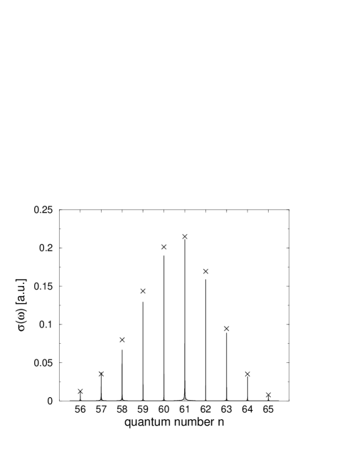
FIG. 1.: Semiclassical spectrum (full curve) compared to quantum spectrum (crosses) with parameters ${\bf r}_{0}=(0,0,6000\,a.u.)$, ${\bf p}_{0}=(0,0,0)$ and $\gamma^{2}=2/600^{2}$.

FIG. 2.: Semiclassical spectrum (full curve) compared to quantum spectrum (crosses) with parameters ${\bf r}_{0}=(0,0,20\,a.u.)$, ${\bf p}_{0}=(0,0,0)$ and $\gamma^{2}=0.1$.

FIG. 3.: Lower panel: Semiclassical spectrum (full curve) compared to quantum spectrum (crosses) with parameters ${\bf r}_{0}=(0,0,2500\,a.u.)$, ${\bf p}_{0}=(0,0,0)$ and $\gamma^{2}=0.0001$; upper panel: average normalized angular momentum according to Eq. (17) (circles).

FIG. 4.: Lower panel: Semiclassical spectrum (full curve) compared to quantum spectrum (crosses) with parameters ${\bf r}_{0}=(0,0,6000\,a.u.)$, ${\bf p}_{0}=(0,0.0075,0)$ and $\gamma^{2}=2/600^{2}$; upper panel: average normalized angular momentum according to Eq. (17) (circles).

REFERENCES

- [1] K. G. Kay, J. Chem. Phys. 101, 2250 (1994).
- [2] F. Großmann, Chem. Phys. Lett. 262, 470 (1996).
- [3] B. W. Spath and W. H. Miller, Chem. Phys. Lett. 262, 486 (1996).
- [4] S. Garashchuk and D. Tannor, Chem. Phys. Lett. 262, 477 (1996).
- [5] M. F. Herman and E. Kluk, Chem. Phys. 91, 27 (1984).
- [6] K. G. Kay, J. Chem. Phys. 100, 4377 (1994).
- [7] F. Großmann, Phys. Lett. A243, 243 (1998).
- [8] I. M. Suárez Barnes, M. Nauenberg, M. Nockleby and S. Tomsovic, Phys. Rev. Lett. 71, 1961 (1993); J. Phys. A 27, 3299 (1994).
- [9] R. S. Manning and G. S. Ezra, Phys. Rev. A 50, 954 (1994).
- [10] M. R. Wall and D. Neuhauser, J. Chem. Phys. 102, 8011 (1995).
- [11] V. A. Mandelshtam and H. S. Taylor, Phys. Rev. Lett. 78, 3274 (1997); J. Chem. Phys. 107, 6756 (1997).
- [12] H. Kleinert, Path integrals in quantum mechanics, statistics, and polymer physics, 2nd ed., (World Scientific, Singapore, 1995).