Ionization dynamics in intense pulsed laser radiation. Effects of frequency chirping.

Abstract

Via a non–perturbative method we study the population dynamics and photoelectron spectra of Cs atoms subject to intense chirped laser pulses, with gaussian beams. We include above threshold ionization spectral peaks. The frequency of the laser is near resonance with the 6s-7p transition. Dominant couplings are included exactly, weaker ones accounted for perturbatively. We calculate the relevant transition matrix elements, including spin–orbit coupling. The pulse is taken to be a hyperbolic secant in time and the chirping a hyperbolic tangent. This choice allows the equations of motions for the probability amplitudes to be solved analytically as a series expansion in the variable $u=(\tanh(\pi t/\tau)+1)/2$, where $\tau$ is a measure of the pulse length. We find that the chirping changes the ionization dynamics and the photoelectron spectra noticeably, especially for longer pulses of the order of $10^{4}$ a.u. The peaks shift and change in height, and interference effects between the 7p levels are enhanced or diminished according to the amount of chirping and its sign. The integrated ionization probability is not strongly affected.

• Physics Dept., New York University, New York, NY 10003, USA

1 Introduction

The ionization of an atom by a pulse of laser radiation is a fundamental process which is only well understood in certain regions of intensity, frequency and pulse length. The regime which is best understood is when perturbation theory may be applied, that is where the intensity is very low, the frequency not too low, and the pulse very long and constant or quasi constant in electric field amplitude (see e.g. [1]). In particular, the amplitude of the initial state is approximately equal to one for the entire duration of the process.

Since the intensity of the radiation field is nowadays often comparable with the internal field of the atom, perturbation theory is inadequate. Perturbation theory also breaks down at lower intensities if the field frequency is close to a resonance, or if saturation occurs. Thus, the applicability of lowest–order theory is limited to non–resonant absorption. Resonance effects involving intermediate states can make the picture much more complicated and must be described by a theory which allows for strong signals.

Another degree of complexity appears when the length of the pulse is shortened (less than $10^{-13}$ s) : the peaks shift, widen and develop substructures. For example the energies of the atomic states shift by amounts, which, to the first non–vanishing order, are proportional to the intensity of the laser field (A.C. Stark effect). Thus an intermediate atomic level can shift in such a way that it comes into resonance at certain times during the laser pulse.

The above processes have been approached theoretically in a few different ways and described in different, not always compatible languages, often corresponding to non–identical experimental situations.

Some calculations are based on the application of Floquet theory [2, 3], a semiclassical approach which takes advantage of the temporal periodicity of the Hamiltonian.

Other theories are based on the Keldysh–Faisal–Reiss (KFR) model [4, 5]. In an approximation originally due to Keldysh and developed by Reiss, the exact final state of the electron is replaced by solutions of the Schrödinger equation for a free electron in a laser field. The Keldysh approximation may be quite successful if the atomic potential is of very short range, at least for the position of spectral peaks. However KFR treatments have not fared particularly well in quantitative comparisons with experiments specifically designed to test their predictions regarding ATI electron spectra [6].

Another type of method is the essential states approach [7], which focuses on continuum–continuum interactions. States are called “essential” if they are populated during the entire process of ATI. Such a theory allows simple analytical solutions, provided some assumptions are made. These include the rotating wave approximation, the treatment of transitions into the continuum from the ground state as a direct non–resonant multiphoton process, and the assumption that all transition matrix elements between states belonging to different continua have one of several simple analytic forms.

In a number of studies, the time–dependent Schrödinger equation has been solved by direct numerical integration for model atoms. Studies have been done both on one–dimensional atoms (e.g. [8, 9]), and more realistic models [10], using various approximations. One of the limitations of this hard numerical approach is the time required for these simulations and attendant lack of flexibility. For example the space–temporal shape of the laser beam can only be roughly taken into account. This approach does not offer great insight into the physics, but since the experimental results can vary greatly even for very similar experiments, these results can be looked at as numerical experiments against which one can further test model theories.

The above–mentioned models usually represent only some important features of real systems and make simplifying assumptions. Many studies are done for constant fields, or cannot describe processes of resonant–enhanced multiphoton ionization. The same can be said about numerical computations, very sophisticated and time consuming even for one–dimensional atoms. They only partially contribute to a full understanding of the processes.

Due to the complexities involved in the dynamics of the interaction of an atom with strong short laser pulses, it is useful to try to unveil such dynamics using a model which is both realistic and offers a simple physical interpretation.

We report on a model of the system which is solvable, at least partially, by analytical methods, since these generally allow greater insight than a direct numerical integration. This also reduces the computer effort per parameter set, thus permitting the integration over spatial profiles, where many repetitions are needed.

The work is performed in the semiclassical approximation which has given very good results in the past and is justified given the high intensity of the radiation field. Furthermore the electric dipole approximation is indeed almost always valid at optical frequencies.

A starting point is the Rosen–Zener problem [11, 12, 13]. In this problem a two–level atom is subject to a pulse whose amplitude that varies in time as a hyperbolic secant. Such problem can be solved analytically via a transformation of the time variable $t$ to the “compressed time” $u=(\tanh(\pi t/\tau)+1)/2$. The solutions are hypergeometric functions.

Our model can be regarded as an extension of the basic Rosen–Zener problem to an atom with more that two active levels, including coupling to the continuum, to model ATI, and chirping of the laser.

By using an expansion of the wave function in the amplitudes of atomic states that are most relevant to the dynamics of the system, one obtains a simplification that allows one to get a clearer picture of what is going on during the interaction. These levels are those most strongly coupled to the ground state, and others coupled to that group. In other words, we use a truncated spectral representation of the wave function, which considers only the atomic states most strongly mixed with the ground state and includes the contribution of the remaining levels approximately.

In the application of the method we focus on the cesium atom, both because it is advantageous theoretically, since many of the atomic parameters involved have already been calculated in the literature, and it is also an element which is accessbile to experimental analysis.

We are interested in studying ATI, thus the coupling of the bound states to the continua corresponding to the second ionization peak will also be included. We also include frequency chirping in the laser pulse and account for a Gaussian spatial shape.

Section 2 introduces the model for the physical system under study and the method of solution of the time dependent Schrödinger equation is discussed. In section 3 the atomic and laser parameters are characterized. The results of the simulations are presented in section 4 and the conclusions in section 5.

2 Alkali Atoms in Strong Pulsed Resonant Laser Radiation

In this section we describe the theoretical model and the solutions of the corresponding equations of motion. Atomic units are used throughout this article, that is, one takes $e=m=\hbar=1$ a.u.

2.1 The Model

The system under study consists of an alkali atom, which has a single active electron, interacting with pulsed laser radiation. The electron wave function is expanded in the basis of unperturbed energy eigenstates. To simplify the notation the atomic levels are labeled with a single index, which stands for the standard set of quantum numbers completely identifying the electron state. In this notation the electron wave function can be written as

$$|\Psi(t)>=\sum_{n}c_{n}(t)\exp(-i\omega_{n}t)|n>$$ (1)

where the sum spans the bound states and includes an integration over the continuum.

As noted in the introduction, we make the dipole approximation. In addition, the work is done in the length gauge because it can be argued that it gives a better approximation than the velocity gauge when a truncated basis is used to represent the electronic wave function. If the unperturbed potentials are velocity–independent, the momentum matrix elements are related to the dipole matrix elements by $<n|p|0>=i(E_{n}-E_{0})<n|z|0>$. Thus, the momentum matrix elements decrease more slowly with the energy difference than do the length ones. Then, calculating multiphoton transition amplitudes, in the sum over intermediate states, the velocity gauge weighs states more distant in energy more than the length gauge does and the sum converges more slowly. Thus, a truncated basis using states close to resonance is a better approximation in the length gauge. The Hamiltonian in length gauge is given by

$$H=H_{0}+{\bf E}\cdot{\bf r}$$ (2)

where $H_{0}$ is the unperturbed atomic Hamiltonian.

The incident laser field can be written as

$${\cal E}(t)=2E(t)\cos(\Omega t+\alpha(t))$$ (3)

where $E$ represents the pulse shape and $\alpha$ the frequency chirping, i.e. a time-dependence of the optical frequency. Experimentally this effect usually accompanies the creation of short laser pulses, and to the best of our knowledge, has not been included in previous work on ionization.

We consider photoionization processes in which the laser frequency is nearly resonant with the transition between the ground and some excited levels, so that ionization is possible from the excited states through the absorption of one photon. Specifically we will study cesium subject to laser light in resonance with the 6s–7p transition. The level scheme is shown in Fig. 1.

If the frequency of the light is close to resonance for the transition between the ground state and some excited levels, the dynamics of the electron will be dominated by the corresponding contributions of such levels. In addition, other levels should be retained if, although nonresonant, they have a very strong coupling with the ground state. We call all these states “relevant” states and solve for their effect exactly. In addition we can correct for the contribution of the further atomic levels in a perturbative way, calculating the energy shifts they induce on the relevant states. We use the rotating wave approximation, since we are interested in optical frequencies, a regime where such an approximation is typically excellent.

We make the Weisskopf–Wigner approximation so that the coupling between the bound states and the continuum levels is modeled by decay coefficients and level shifts. This can be done also for the processes corresponding to excess photon absorption (i.e. ATI).

We now give an outline of the derivation of the equations of motion for the probability amplitude using the afore mentioned approximations. Using Eqs.(1) and (2) and assuming the electric field to be polarized in the $\hat{z}$ direction, the time–dependent Schrödinger equation yields:

$$i\dot{c}_{m}={\cal E}(t)\sum_{n}\kappa_{mn}\exp(-i\omega_{nm}t)c_{n}(t)$$ (4)

where $\omega_{mn}\equiv\omega_{m}-\omega_{n}$ and $\kappa_{mn}\equiv<m|z|n>$. Initially the atom is its ground state. Since we assume that the non–relevant states and the continuum are going to be scarcely populated, we can treat them perturbatively, so that for one of such states, $k$:

$$c_{k}(t)\approx-i\sum_{n}\kappa_{kn}\int_{-\infty}^{t}dt^{\prime}{\cal E}(t^{\prime})\exp(-i\omega_{nk}t^{\prime})c_{n}(t^{\prime}),$$ (5)

The sum is over the relevant states. We then substitute the above expression into the equation of motion for the relevant state $m$ and perform the time integration by parts, we get a term containing a time derivative which we can neglect in the Weisskopf–Wigner approximation.

Further we neglect terms containing factors such as $\exp(2i\Omega t)$. We then assume that $\Omega\approx\omega_{nm}$ (quasi–resonant approximation), keep only the resonant term explicitly and the first non–vanishing off–resonance correction. Finally, we set $c_{m}=a_{m}\exp(-i\lambda_{m}\int_{-\infty}^{t}dt^{\prime}E^{2}(t^{\prime}))$.

With these approximations the equations of motion for the probability amplitudes $\{a_{i},i=1,N\}$ are

$$\frac{da_{1}}{dt} = -i\sum_{l=2}^{N}\kappa_{1l}E(t)\exp\left[i(\Delta_{1l}t+\phi_{1l}(t)+\alpha(t))\right]a_{l}(t),$$ (6)

$$\frac{da_{m}}{dt} = -i\kappa_{1m}E(t)\exp\left[-i(\Delta_{1m}t+\phi_{1l}(t)+\alpha(t))\right]a_{1}(t)$$

$$-[\gamma_{m}E(t)^{2}/2]a_{m}(t),$$

$$\phi_{lj}(t) \equiv (\lambda_{l}-\lambda_{j})\int_{-\infty}^{t}dt^{\prime}E(t^{\prime})^{2}$$ (8)

where $\kappa_{ij}$ are the coupling coefficients between levels $i$ and $j$, i.e. $\kappa_{ij}=<i|z|j>$, $\Delta_{ij}\equiv\Omega-(\omega_{j}-\omega_{i})$ is the detuning from the transition frequency, the $l$ summation is over all excited states, $\lambda_{j}$ is the Stark coefficient for the $j$th level and $\gamma_{j}E(t)^{2}$ is the decay rate, i.e. $\gamma_{j}=2\pi|\kappa_{jk}|^{2}$, with $\omega_{j}-\omega_{k}=\Omega$. Since we will consider only a small range of frequencies near resonance, we assume that the decay coefficients are constant over this energy interval. The explicit Stark shift terms include contributions from all other levels and also the non–resonant contribution from the same level, which provides a correction to the rotating wave approximation. For an excited level $j$, the Stark shift is given by

$$\lambda_{j}=\frac{|z_{j1}|^{2}}{\Omega+\omega_{j1}}+{\sum_{k}}^{\prime}\left(\frac{|z_{jk}|^{2}}{\Omega+\omega_{jk}}+\frac{|z_{jk}|^{2}}{\omega_{jk}-\Omega}\right),\>(j\neq 1)$$ (9)

and by

$$\lambda_{1}=\sum_{n}\frac{|z_{1n}|^{2}}{\Omega+\omega_{1n}}+{\sum_{k}}^{\prime}\left(\frac{|z_{1k}|^{2}}{\Omega+\omega_{1k}}+\frac{|z_{1k}|^{2}}{\omega_{1k}-\Omega}\right)$$ (10)

for the ground state, where the sum over $k$ includes the principal value of the integral over the continuum states as well as the bound states not explicitly considered in the model, while the sum over n spans the “relevant” states. The equations for the continuum amplitude for a state of frequency $\omega_{\kappa}$ are

$$\frac{da_{k}}{dt}=-iE(t)\sum_{l=2}^{N}\kappa_{lk}\exp\left[-i\left(\Delta_{lk}t+\phi_{lk}(t)+\alpha(t)\right)\right]a_{l}(t)$$ (11)

for the first ionization peak, and

$$\frac{da_{q}}{dt}=-iE(t)^{2}\sum_{l=2}^{N}\chi_{lq}\exp\left[-i\left(\Delta^{\prime}_{lq}t+\phi_{lq}(t)+\alpha(t)\right)\right]a_{l}(t)$$ (12)

for the second ionization peak (ATI). Here the detuning is given by $\Delta^{\prime}_{lq}=2\Omega-(\omega_{q}-\omega_{l})$, the Stark coefficient $\lambda_{k}\equiv 1/\Omega^{2}$ and $\chi_{lq}$ is the two–photon coupling between the bound state $l$ and the continuum state $q$ (see Eq.(27).

In the above equations we consider only the lowest order terms in the field, i.e. cross terms corresponding to the absorption of one photon from an excited state and re–emission to a different one are neglected. A few test runs have shown this contribution to be negligible. In the same manner, we neglect the effect of the decay rate to the second continuum on the equations of motion for the excited bound states. One could readily allow for this effect, but it proves to be negligible for the conditions we encounter. We also neglect the process involving absorption of two photons from an excited state and re–emission of one photon to a continuum state.

While the equations can be generalized to any number of excess photons absorbed, we will consider only the first two peaks.

To enable the analysis to be carried out in closed form, we chose a field envelope in the shape of a hyperbolic secant and a frequency chirp proportional to a hyperbolic tangent :

$$E(t)=\sqrt{I_{0}}\mbox{$\rm{sech}(\pi t/\tau)$},\mskip 5.0mu plus 5.0mu\alpha(t)=\beta\int_{-\infty}^{t}dt^{\prime}\tanh(\pi t^{\prime}/\tau)$$ (13)

where the characteristic time, $\tau$, of the amplitude modulation is large compared to $1/\Omega$. This allows a solution in the form of a power series in the compressed time, which we will define below.

2.2 Solution of the Equations of Motion

In order to solve the equations of motion for the probability amplitude given in the previous section, we first let

$$b_{1} = a_{1}$$ (14)

$$b_{j} = \exp[i(\Delta_{1m}t+\phi_{1j}(t)+\alpha(t))]a_{m},$$ (15)

where $m=2,3,\dots,N$. The equations of motion for the new $b$ amplitude are

$$\frac{db_{1}}{dt} = -i\sum_{l=2}^{N}\kappa_{1l}E(t)b_{l}(t),$$ (16)

$$\frac{db_{m}}{dt} = -i\kappa_{1m}E(t)b_{1}(t)-\frac{\gamma_{m}E(t)^{2}}{2}b_{m}(t)$$ (17)

$$+i\left(\Delta_{1m}+\dot{\phi}_{1m}(t)+\dot{\alpha}(t)\right)b_{m},$$

where

$$\dot{\phi}_{lm} = (\lambda_{l}-\lambda_{m})E(t)^{2},$$ (18)

$$\dot{\alpha}(t) = \beta\tanh(\pi t/\tau).$$ (19)

The continuum probability amplitudes are found by formally integrating the corresponding equations of motion:

$$a_{k}(t)=-i\int_{-\infty}^{t}dt^{\prime}E(t^{\prime})\sum_{l=2}^{N}\kappa_{lk}\exp\left[-i\left(\Delta_{1k}t^{\prime}+\phi_{1k}(t^{\prime})+\alpha(t^{\prime})\right)\right]b_{l}(t^{\prime})$$ (20)

for the first ionization peak, and

$$a_{q}(t)=-i\int_{-\infty}^{t}dt^{\prime}E(t^{\prime})^{2}\sum_{l=2}^{N}\chi_{lq}\exp\left[-i\left(\Delta^{\prime}_{1q}t^{\prime}+\phi_{1k}(t^{\prime})+\alpha(t^{\prime})\right)\right]b_{l}(t^{\prime})$$ (21)

for the second ionization peak (ATI).

Letting $u\equiv(\tanh(\pi t/\tau)+1)/2$ and expanding the bound state amplitudes in a power series in $u$, we find :

$$b_{1}=\sum_{n=0}^{\infty}\alpha_{n}u^{n},\mskip 5.0mu plus 5.0mub_{j}=\sum_{n=0}^{\infty}\beta_{n}^{(j)}u^{n}\mbox{$\rm{sech}(\pi t/\tau)$}\equiv\sum_{n=0}^{\infty}\mu_{n}^{(j)}u^{n}.$$ (22)

The expansion coefficients can be calculated through the following recursion equations:

$$(j+1)\alpha_{j+1}+i\frac{2\tau}{\pi}E_{0}\sum_{l=2}^{N}\kappa_{1l}\beta_{j}^{(l)}=0$$ (23)

$$\left[n+{1\over 2}-i\frac{\tau}{2\pi}(\Delta_{1j}-\beta)\right]\beta_{n}^{(j)}=\left[n+i\frac{\tau}{2\pi}(4\lambda_{1j}I_{0}+2\beta)-\right.$$

$$\left.2\gamma_{j}E_{0}^{2}\frac{\tau}{2\pi}\right]\beta_{n-1}^{(j)}+(-i\lambda_{1j}I_{0}4\frac{\tau}{2\pi}+2\gamma_{j}I_{0}\frac{\tau}{2\pi})\beta_{n-2}^{(j)}-i\frac{\tau}{2\pi}\kappa_{1j}\sqrt{I_{0}}\alpha_{n}.$$ (24)

Using the expansion in powers of $u$ in the formula for the continuum amplitude and integrating term by term, we get

$$a_{k} = -i\frac{E_{0}\tau}{\pi}2^{i\beta\tau/\pi}\sum_{n=0}^{\infty}\sum_{l=2}^{N}\mu_{n}^{(l)}\kappa_{lk}$$ (25)

$$\times B\left(\frac{1}{2}+i\frac{\tau}{2\pi}(\Delta_{1k}+\beta),n+1-i\frac{\tau}{2\pi}(\Delta_{1k}+\beta)\right)$$

$$\times {}_{1}\!F_{1}\left(n+1-i\frac{\tau}{2\pi}(\Delta_{1k}-\beta),\frac{3}{2}+n+i\frac{\tau}{2\pi}2\beta,-i(\lambda_{1}-\lambda_{k})I_{0}\frac{2\tau}{\pi}\right)$$

and

$$a_{q} = -i\frac{I_{0}\tau}{\pi}4^{i2\beta\tau/\pi}\sum_{0}^{\infty}\sum_{l=2}^{N}\mu_{n}^{(l)}\chi_{lq}$$ (26)

$$\times B\left(1+i\frac{\tau}{2\pi}(\Delta^{\prime}_{1q}+2\beta),n+\frac{3}{2}-i\frac{\tau}{2\pi}(\Delta_{1k}-2\beta)\right)$$

$$\times {}_{1}\!F_{1}\left(n+\frac{3}{2}-i\frac{\tau}{2\pi}(\Delta_{1k}-\beta),\frac{5}{2}+n+i\frac{\tau}{2\pi}4\beta,-i(\lambda_{1}-\lambda_{k})I_{0}\frac{2\tau}{\pi}\right).$$

where $B$ is the beta function and ${}_{1}F_{1}$ the confluent hypergeometric function. These results have been implemented both with Mathematica and Fortran programs. Mathematica allows an arbitrary amount of precision, but it is about a hundred times slower than the Fortran version. For fields up to $10^{-5}$ atomic units and pulse lengths up to $10^{4}$ atomic units Fortran’s double precision proved to yield the same results as the Mathematica code.

3 Atomic and Laser Parameters

The model atom is characterized by several coupling and decay constants and level shifts, which need to be evaluated. Coefficients for one–photon transitions are given by the matrix elements $\kappa_{fi}=<f|z|i>$ and the Stark–shift parameters $\lambda_{j}$ by Eq.(9) and (10). The two–photon coupling between the excited states and the continuum is given by $\chi_{fi}$ in Eq.(27). For the case of the cesium atom the above parameters are already available in the literature (see e.g. [13]) except for the two–photon couplings above threshold.

We choose the laser field to be linearly polarized in the z direction and of frequency such that we can model this problem accurately with the retention of only four excited states, those of the 6p and the 7p doublets. The 7p states are quasi resonant, while the 6s-6p oscillator strengths are orders of magnitude larger than any other coupling to the ground state. Thus, retaining the 6p doublet takes non resonant ionization into account with negligible error. The level scheme is shown in Fig. 1. We take the ground state energy to be equal to zero. The ionization potential of cesium is 3.89 eV.

In Table 1, we list the energy levels and Stark shift coefficients of the relevant states of cesium.

Table 1: Energy levels and Stark shift coefficients of the relevant states of cesium

• State	Energy (a.u.)	Stark Shifts (a.u.)
  62s1/2	$\omega_{1}$=0.0	$\lambda_{1}$= -76.93493
  62p1/2	$\omega_{2}$=0.050931	$\lambda_{2}$= 159.221
  62p3/2	$\omega_{3}$=0.053456	$\lambda_{3}$= 232.48688
  72p1/2	$\omega_{4}$=0.0992	$\lambda_{4}$= 64.3317
  72p3/2	$\omega_{5}$=0.1000	$\lambda_{5}$= 386.861

The decay parameters were calculated in [13] by the method developed by Burgess and Seaton [14], the matrix elements coupling of the bound states were calculated using the quantum defect method and the non resonant couplings were calculated using data found in Stone [15]. In the present work we also need the coupling coefficients between the bound states and the continua associated with the second ionization. This corresponds to the absorption of 2 photons from the excited states, when the absorption of 1 photon is permitted (that is, we have “above threshold ionization”).

3.1 Calculation of the coupling to ATI channels

One needs to evaluate terms like :

$$\chi_{fi}=\lim_{\eta\to 0}\sum_{k}\frac{z_{fk}z_{ki}}{\Omega+\omega_{i}-\omega_{k}+i\eta}.$$ (27)

The sum spans all intermediate bound and continuum states. Here $\Omega$ is the laser frequency and $\omega_{i}$ is the energy of the initial bound state. The $\eta$ in the denominator was included because above threshold ($\Omega>|\omega_{i}|$) the denominator vanishes when $\omega_{n}=\omega_{i}+\Omega$. The small imaginary part prescribes the correct boundary conditions for a field adiabatically turned on in the remote past.

Several methods have been developed to calculate transition amplitudes involving infinite sums over intermediate states. For alkali atoms, quantum defect theory and model potentials have been used as weel as truncated summations over a finite number of states. Most calculations have taken the laser frequency to be below threshold.

We used a method based on the solution of an Inhomogeneous Differential Equation (IDE), which is equivalent to performing the sums over the entire spectrum of bound and continuum intermediate states. In this formulation we have

$$\chi_{fi}=<\Psi_{f}|z|\tilde{\Psi}_{i}>$$ (28)

where $|\tilde{\Psi}_{i}>$ is the solution of

$$[H_{0}-\omega]\tilde{\Psi}_{i}(\mbox{\bf r})=-z\Psi_{i}(\mbox{\bf r}),$$ (29)

with $\omega=\omega_{i}+\Omega$, which is a positive quantity for ATI.

This method, which is based on numerical computations in the framework of the central field approximation has a wider range of applicability than the afore mentioned analytical methods, and also leads to accurate results.

The central potential we used is calculated in [16] using the Hartree–Fock–Slater approximation. We add a spin–orbit interaction of the form

$$V_{SO}(r)={\bf\hat{L}\cdot\hat{S}}\frac{\alpha^{2}}{2r}\frac{dV}{dr}$$ (30)

where $V$ is the Hartree–Fock potential calculated without spin–orbit interaction. We work in the SLJM representation.

The initial state wave function $\Psi_{i}$, represents a state identified by the quantum numbers $i\equiv\{n_{i},j_{i},l_{i},m_{i}\}$ and can be expressed in terms of the product of a radial function and a generalized spherical harmonic :

$$\Psi_{i}(r,\hat{\Omega})=R_{i}(r){\cal Y}(j_{i},l_{i},m_{i};\hat{\Omega}).$$ (31)

We look for a solution in terms of a superposition of eigenstates of the total and orbital angular momentum.

$$\tilde{\Psi}_{i}(\omega,r,\hat{\Omega})=\sum_{j,l,m}\tilde{R}_{i}(\omega,j,l,m;r){\cal Y}(j,l,m;\hat{\Omega}).$$ (32)

Projecting Eq.( 29) on state $|jlm>\equiv{\cal Y}(j,l,m;\hat{\Omega}$), we obtain :

$$[H_{0}-\omega]\tilde{R}_{i}(\omega jlm;r)=-<jlm|\cos\theta|j_{i}l_{i}m_{i}>R_{n_{i}}(j_{i}l_{i}m_{i};r)r.$$ (33)

The matrix element of $\cos\theta$ can be calculated by an application of the Wigner–Eckart theorem [17] :

$$<l^{\prime}j^{\prime}m^{\prime}|r^{q}|ljm> = (-1)^{3/2+j^{\prime}+j-m^{\prime}-l_{>}}\sqrt{l_{>}}[(2j^{\prime}+1)(2j+1)]^{1/2}r$$ (38)

$$\times\left(\begin{array}[]{ccc}j^{\prime}&1&j\\ -m^{\prime}&q&m\end{array}\right)\left\{\begin{array}[]{ccc}l^{\prime}&j^{\prime}&1/2\\ j&l&1\end{array}\right\}$$

where $r^{0}=z,r^{\pm 1}=\mp 1/2(x\pm iy)$ and $l_{>}\equiv\max(l,l^{\prime})$. In our case $q=0$.

For cesium the ground state is 6S_1/2. Since the final result will not depend on the projection of the spin, we can pick a state with m_S=1/2 without loss of generality, i.e. n= 6, l=0, j=1/2, m=1/2. Since the interaction $z$ conserves the spin and m_l, m will always be equal to $+1/2$ and we will drop it in subsequent formulas.

After the absorption of one photon from the ground state, the electron will be in a state p_1/2 or p_3/2. Since we will consider laser frequencies close to the transition frequency between the ground state and the 7p’s states, our atomic model will consider these states explicitly, and as noted, also the 6p’s, because their coupling to the ground state is very large. Thus, the initial state for the transition to the continuum via the absorption of 2 photons can be any of the 6p’s or 7p’s states. Let $P(r)\equiv rR(r)$, then

$$\left[-\frac{d^{2}}{dr^{2}}+\frac{l(l+1)}{r^{2}}+V(jl;r)-\omega\right]\tilde{P}_{i}(\omega jl,r)=$$

$$-<jl{1\over 2}|\cos\theta|j_{i}l_{i}{1\over 2}>rP_{n}(j_{i},l_{i};r).$$ (39)

where $R_{n}$ is an eigenstate of the unperturbed atom with $n=6,7$, $j=1/2,3/2$ and $l_{i}=1$.

First we solve the unperturbed Schrödinger equation to calculate the initial bound state which enters in the inhomogeneous term of Eq.(39). This is done through a modification of Herman and Skillman’s code  [16] to include spin orbit interaction.

We solve Eq.(39) numerically using Numerov’s method (see e.g. [18]) integrating outward from the origin. The boundary conditions require the solution to be zero at the origin and to be an outgoing wave for large $r$. We start the integration using a Taylor expansion around the origin. In general the solution obtained does not satisfy the boundary conditions at infinity, so we add a solution of the homogeneous equation such that the combination satisfies the boundary conditions at infinity. The coefficients of the combination are determined using the asymptotic expansion of Coulomb functions. In fact, at a large distance from the origin, the potential approaches $-1/r$ so that the solutions have the form of phase–shifted Coulomb waves.

The transition matrix to a final state $|\omega_{q},l_{f},j_{f}>$ is given by

$$<\omega_{f},l_{f},j_{f}|z|\tilde{\Psi}_{i}({\omega})>=\sum_{l^{\prime}j^{\prime}}<\omega_{f},l_{f},j_{f}|z|l^{\prime}j^{\prime}><l^{\prime}j^{\prime}|\tilde{\Psi}_{i}(\omega)>$$ (40)

$$=\sum_{l^{\prime}j^{\prime}}\int drrP_{\omega_{f}}(j_{f},l_{f};r)\tilde{P}_{i}(\omega j^{\prime}l^{\prime};r)<j_{f}l_{f}|\cos(\theta)|jl>.$$

The radial integral is calculated by dividing the integration range in two parts. The integration is done numerically up to a certain distance $R_{\max}$. The remaining integral to infinity is evaluated using an expansion in terms of inverse powers of $r,n$ and, whose asymptotic expansion is given in [19] as

$$F_{l}(r) = f(r)\cos\theta_{l}-g(r)\sin\theta_{l},$$ (41)

$$G_{l}(r) = f(r)\sin\theta_{l}+g(r)\cos\theta_{l},$$ (42)

$$\theta_{l} = kr+\ln(2kr)/k-l\pi/2+\sigma_{l},$$ (43)

$$\sigma_{l} = \arg\Gamma(l+1-i/k),$$ (44)

where $f$ and $g$ can be expanded in inverse powers of $kr$ for large $kr$ ($k=\sqrt{2E}$). The resulting integrals have an analytical form, which maybe written as

$$\int_{R}^{\infty} dx\exp(iax)x^{\lambda-ib}=$$ (45)

$$-\frac{\exp(iaR)}{ia}R^{\lambda-ib}\left(1-\frac{\lambda-ib}{iaR}+\frac{(\lambda-ib)(\lambda-ib-1)}{(iaR)^{2}}-...\right).$$

3.2 Transition Amplitudes for Cesium and Laser Parameters

By virtue of the angular momentum selection rules, the 6s ground state couples to the 6p and 7p states, while the p states couple via one–photon absorption to the s and d continuum channels and to the p and f continuum channels via two–photon absorption. Fig. 2 presents a diagram of the various ionization channels considered in this study and Tabs. 2, 3 and 4 give the corresponding coefficients calculated with the methods described in the previous section.

Table 2: Coupling coefficients between the ground state and the excited states.

• Parameter	Value (a.u.)
  $\kappa_{12}$	-1.81
  $\kappa_{13}$	-2.56
  $\kappa_{14}$	0.11
  $\kappa_{15}$	0.23

Table 3: Decay rates from the excited states to the continuum channels via one–photon transitions, for a laser frequency quasi resonant with the 6s-7p transition. The corresponding coupling coefficients are given by $\sqrt{\gamma_{ij}/2\pi}$.

• Parameter	Value (a.u.)
  $\gamma_{21}$	117.5878	(6P${}_{1/2}\rightarrow{\rm S}_{1/2}$)
  $\gamma_{22}$	10.45479	(6P${}_{1/2}\rightarrow{\rm D}_{3/2}$)
  $\gamma_{31}$	13.83078	(6P${}_{3/2}\rightarrow{\rm S}_{1/2}$)
  $\gamma_{32}$	10.41901	(6P${}_{3/2}\rightarrow{\rm D}_{3/2}$)
  $\gamma_{33}$	93.11069	(6P${}_{3/2}\rightarrow{\rm D}_{3/2}$)
  $\gamma_{41}$	37.4357	(7P${}_{1/2}\rightarrow{\rm S}_{1/2}$)
  $\gamma_{42}$	3.50958	(7P${}_{1/2}\rightarrow{\rm D}_{3/2}$)
  $\gamma_{51}$	3.33084	(7P${}_{3/2}\rightarrow{\rm S}_{1/2}$)
  $\gamma_{52}$	3.003428	(7P${}_{3/2}\rightarrow{\rm D}_{3/2}$)
  $\gamma_{53}$	26.8404	(7P${}_{3/2}\rightarrow{\rm D}_{5/2}$)

Table 4: Coupling parameters to the continuum via two–photon transitions (ATI peak); $i$ is the imaginary unit.

• Parameter	Value (a.u.)
  $\chi_{24}$	$1972-2916i$	(6P${}_{1/2}\rightarrow{\rm P}_{1/2}$)
  $\chi_{25}$	$-960+484i$	(6P${}_{1/2}\rightarrow{\rm P}_{3/2}$)
  $\chi_{26}$	$-2568+4759i$	(6P${}_{1/2}\rightarrow{\rm F}_{5/2}$)
  $\chi_{34}$	$-616-884i$	(6P${}_{3/2}\rightarrow{\rm P}_{1/2}$)
  $\chi_{35}$	$3188+2068i$	(6P${}_{3/2}\rightarrow{\rm P}_{3/2}$)
  $\chi_{36}$	$844+456i$	(6P${}_{3/2}\rightarrow{\rm F}_{5/2}$)
  $\chi_{37}$	$-2672-1356i$	(6P${}_{3/2}\rightarrow{\rm F}_{7/2}$)
  $\chi_{44}$	$106.8+29i$	(7P${}_{1/2}\rightarrow{\rm P}_{1/2}$)
  $\chi_{45}$	$64-15.9i$	(7P${}_{1/2}\rightarrow{\rm P}_{3/2}$)
  $\chi_{46}$	$383.2-460i$	(7P${}_{1/2}\rightarrow{\rm F}_{5/2}$)
  $\chi_{54}$	$62.8-26.84i$	(7P${}_{3/2}\rightarrow{\rm P}_{1/2}$)
  $\chi_{55}$	$-142.8+23.92i$	(7P${}_{3/2}\rightarrow{\rm P}_{3/2}$)
  $\chi_{56}$	$-65.6+79.6i$	(7P${}_{3/2}\rightarrow{\rm F}_{5/2}$)
  $\chi_{57}$	$199.2-235.6i$	(7P${}_{3/2}\rightarrow{\rm F}_{7/2}$)

In this work we are interested in short laser pulses. After the first successful generation of short optical pulses via mode locking with Nd:glass in the sixties, steady progress in generating shorter and shorter pulses was achieved. For a review, see for example [20].

Nowadays the shortest pulses generated directly from a laser can be achieved with Ti:sapphire lasers. These lasers can be used to achieve $10^{-14}$ s pulse generation [21] by using nonlinear effects which induce frequency chirps. Complete compensation of the chirp is not possible with a finite number of linear optical elements.

With these experimental considerations in mind, we will consider laser pulses of durations in the 25-250 fs range, with frequency almost on resonance with the 6s-7p transition. The frequency chirping induced by the compression mechanisms, is characterized by a chirp parameter $\beta$ of the order of $\pi/\tau$. The parameters characterizing the laser beam are thus frequency, chirp parameter and intensity. The temporal dependence of the pulse is given by Eqs.(2.3) and (2.16). We will consider intensities in the range $10^{-7}-10^{-4}$a.u., and pulse lengths of $10^{3}-10^{4}$a.u., with chirp parameters $\beta\approx\pi/\tau$.

4 Ionization Dynamics of Cesium

In this section, the method described in section 2 is applied to the case of cesium, using the atomic and laser parameters calculated and listed in section 3. We will consider three different regimes according to the intensity of the laser beam and the case of Gaussian beams. The ‘atomic’ unit of intensity here is $1.4\times 10^{17}$ W/cm² – four times the unit used by many other authors.

4.1 Weak Field Limit

The spectrum for weak fields (in the adiabatic limit) is usually a single peak at an energy twice the photon energy above the ground state. In fact, for this case, one expects the final energy of the photoelectron to consist of the Fourier distribution of the pulse squared at an energy consistent with energy conservation. However, with relatively short, weak pulses tuned between the doublet, a double peak structure is found in the s_1/2 or d_3/2 continuum channels but not in the d_5/2 channel. This structure was first reported in [13] and attributed to the interference between the two different ionization paths to the afore mentioned channels, which results in the suppression of the central peak. However the d_5/2 channels can be reached only in one way, through the p_3/2 excited states and thus cannot show any interference effects.

Adler et al. [13] found that one sees a pair of peaks only when the condition $1<|\Delta_{1j}\tau|<10$ is roughly true. This behavior is consistent with the interpretation of such structure as a manifestation of destructive interference between the 7p levels, when the laser is tuned to the middle of the doublet. For very short pulses, the incident radiation’s spectrum covers a wider range of frequencies and the detuning is less significant so that the 7p’s are practically a new single state and the doublet disappears (see Fig. 3). For longer pulses, the central peak forms again and hides the side peaks, which are much smaller. The central peak is about at frequency $\omega_{1}+2\Omega$, while the two side peaks at $\omega_{4}+\Omega$ and $\omega_{5}+\Omega$. The relative heights are correlated with the average populations of the 7P levels during the pulse.

In Fig. 4 we show the spectra of the S_1/2 channel and the the spectra corresponding to the contribution from the 7p states separately, i.e. with no inteference. One can see here that each 7p state contributes to one of the side peaks. The central peak is not resolved, being very close to the side peaks. If there were no interference effects we would not have the dip between the two side peaks. The existence of two peaks is not due do oscillations in the populations, since we find that these do not occur for the intensities we are considering here, as can be seen for example in Fig. 7.

In the ATI peak the double peak structure is usually absent, in fact the mediation of several channels to the first continuum, makes interference effects less likely to occur. For some particular frequencies there is still some structure present in the P_3/2 channel, which is the channel receiving contributions from all first peak channels. See Fig. 5, where we plot ATI spectra for the P channels for different pulse lengths. As for the two–photon peaks, also here the structures are washed out for shorter pulses. In general the ATI peaks are at frequency $\omega_{1}+3\Omega$ and have a bandwidth larger than that of the $\omega_{1}+2\Omega$ peaks. Infact they entail the Fourier transform of the field pulse to the third power, which has a smaller width (in time) than the square of the pulse.

We note that the broadening of the ATI peaks was reported in the experimental results reported in 1992 by Nicklich et al in [22]. The calculation described by these authors did not predict broadening of the higher peaks, however, although their spectra did contain the oscillations similar to those in the experiment, while those oscillations are absent from our work.

The double peak structure is heavily influenced by the presence of chirping in the laser light, especially for the longer pulses in the above range. Varying the strength and the sign of the chirping changes the absolute and relative height of the peaks, see Fig. 6. In fact, the height of the peaks is determined by the amplitudes of the excited states and their phase relationship, which are influenced by a kind of self–induced phase modulation. Thus imposing external phase modulation (through chirping) on these can strongly influence the ionization probability.

The evolution of the population of the bound states also changes appreciably with chirping for the 7p levels which are quasi–resonant with the laser radiation. The 6p levels are only slightly affected (see Fig. 7). Infact the 6p’s are off–resonance and their populations follow the field adiabatically. In addition the relative height of the side peaks is related to the amount of population in the corresponding level. The sign of the chirping determines which levels will have a bigger average population during the pulse and thus the height of the spectral peak. With our conventions a positive chirp corresponds to a pulse whose instantaneous frequency is lower than the carrier frequency at the beginning of the pulse and increases to a value greater than the carrier frequency in the second half of the pulse. Thus the 7p_1/2 is closer to resonance at the beginning of the pulse and starts becoming populated earlier in the pulse. The 7p_3/2 on the contrary becomes populated at a higher rate later during the pulse, when it gets closer to resonance. Thus its average population during the pulse is lower than in the case of chirp free light. The situation is reversed for negative chirping.

4.2 Strong Field Limit

In the previous section we observed that the double peak structure disappears for short pulses. However, Adler et al. [23] have shown that when the pulse is short and the intensity of the beam increased, the spectra again contain a multipeak structure, which is also present when the laser frequency is tuned outside the doublet. Multiple peaks can appear also in the D_5/2 channel. We can see this in Fig. 8, where we plot the channel D_3/2 spectra for different intensities. Increasing the laser intensity we see a multipeak structure emerge, at the same time the populations also start showing oscillations, see Fig. 9.

As noted in the previous subsection, this result confirms that other mechanisms such as Rabi oscillations and Stark shifts play a role in the production of the multipeak structure in strong fields.

As in the case of weak fields, for such short pulses, the influence of chirping is minimal in the second continuum peaks, but it induces visible changes in the population dynamics and the relative peak heights of the doublet.

For long pulses, the chirping causes dramatic changes in the population dynamics and in the spectra of the threshold peaks, see Figs. 10, 11. The ATI peaks are instead not strongly affected as one expects because of the larger linewidth and general lack of structure, as shown in Fig. 12. It appears that chirping enhances or quenches the oscillations in the populations depending if it is an up–chirp or a down–chirp, while the frequency of the oscillation remains the same.

4.3 Gaussian Beams

In actual experiments the laser beam incident upon the atomic sample has an intensity spatial profile, so that the peak field seen by each bound system is a function of its distance from the axis. In weak fields this is not important, since the intensity is merely an overall factor. This is not the case in strong fields, however. Both the total ionization and the electron energy distribution become complicated functions of the optical field strength, as for example, in Fig. 8 in which we see a second peak developing in the D_3/2 channel with increasing intensity.

If the intensity of the field is weak enough to allow the neglect of depletion of the ground state and coupling between the excited states through multiple transition to the ground state and back, then none excited states is affected by the existence of the other ones. In this limit the solution of each bound state amplitude takes the form of the Rosen–Zener solution (see for example [12] and [11]) for a two–level system in which all energy shifts have been neglected. The spectra produced by this expression are identical to those produced by the exact result for weak laser intensities.

We examine for what intensities and pulse lengths perturbation theory breaks down. The evolution of the bound states start to deviate from the typical behavior at weak fields when the peak intensity and pulse length are such that $I_{\max}\tau\approx 10^{-3}$ a.u., for which nonlinear effects start to show. This onset of nonlinear effects seems to be approximately independent of chirping.

In the perturbative regime, the total ionization is proportional to the square of the intensity, since the dominant process is two–photon absorption.

The total ionization probability is not very sensitive to the presence of chirping, (Fig. 13). There is in general a small increase in the ionization rate, which can be attributed to the widening of the pulse bandwidth from the frequency chirp. The scaling parameter is $2I_{\rm max}\tau/\pi$ and the total ionization is practically the same when the length of the pulse or the current $I$ is changed maintaining the scaling parameter constant.

In the figures we show the evolutions of the populations and the spectra as a function of the distance from the center of the laser beam.

Figs. 14 show the total ionization probability and the excited state population after the passage of the pulse, as a function of the distance from the center of the beam. A curve showing the Gaussian shape of the beam spatial profile is shown for reference. We find that in general the total ionization probability roughly follows the intensity profile of the laser beam, while the population of the excited states after the passage of the pulse shows an oscillatory dependence on the laser peak intensity at the location of the atom. Looking at the temporal evolution of the excited states populations one can see that the gradual change is due to the change in the Rabi frequency and the number of oscillations the populations can do during the pulse. As an illustration in Figs. 15 and we show the population of the 7p_3/2 state as a function of the distance from the center of the laser beam without chirping and with chirping. The distance is normalized such that the FWHM of the beam is unity with the laser parameters given in the figure caption. The effect of chirping is mainly to change the height of the oscillations, a chirping of the opposite sign would flatten out the surface of the plot. In Fig. 16 and we show the spectra for the s_1/2 channel for the same set of parameters as Figs. 15 respectively. The presence of chirping here changes the shape and heights of the peaks. One can see that for this intensity and frequency the spectra does not depend in a monotonic way on the intensity. The final spectra will be a spatial average of all these contributions and the final population of the bound states will also change with position. Then in Fig. 17 we show a comparison between the spatially averaged spectra and the spectra at the peak intensity.

5 Conclusion

The goal of this work was to model the dynamics of an atom with a finite number of active levels interacting with short pulse of strong laser light using a non-perturbative approach in the dominant states. It was hoped to strike a balance between the competing needs of realism and numerical simplicity, extending prior analysis to the case of ATI and a “chirped” pulse.

As was done in prior work, we assumed only a few active levels whose coupling to other states was taken into account by means of time–dependent level shifts and decay rates. By assuming a hyperbolic secant pulse shape for the amplitude of the field, and a related form for the frequency modulation, we were able to extend the analytically solvable problem previously reported to the present case. The ATI was accounted for by means of an effective operator, whose coupling strength was obtained from the solution of an in- homogeneous Schrödinger equation.

The model was applied to the cesium atom for light nearly resonant with transitions between the 6s ground state and 7p excited doublet. Coupling to the 6p doublet is also included explicitly, since, even though its frequency is far from resonance, the interaction matrix element is very large. The approach could be further extended to include more atomic levels and a larger number of ATI peaks. Allowance for the temporal profile of the laser beam was made, and the dynamics of the excited state populations and spectra of the ejected electrons were efficiently calculated.

We found that chirping as a great influence on the dynamics of the quasi- resonant states, but much less of an effect on the off resonant states. This transpires because the chirping causes much less of a fractional change in the detuning of the nonresonant states. In fact, it appears that the dominant part of the change produced in the nonresonant amplitudes by the chirping is due to the modification in the ground state amplitude cause by the resonant intermediate couplings.

The effect of chirping is more pronounced for longer pulses. In this case, the pulse has a smaller linewidth the the fractional change due to the chirping is relatively more prominent.

Some of the spectral features, such as double peaks, can change drastically with the chirpings. Those effects in weak fields are due to the interference between the phases of the various atomic amplitudes when the laser is tuned between resonances, and is very sensitive to time dependent frequency shifrts. The interference is enhanced or suppressed depending on the sign and magnitude of the chirp.

The structure of the spectral peaks is quite sensitive to the length of the pulse. The doublet structure disappears for short pulses. The shorter pulses have a broader frequency spectrum, over which the populations dynamics are averaged, thus washing out the deleicate interference effect due to phase modulation.

It is interesting to note that the ATI peaks lack the structure of the principal two–photon peaks, even though both types are generated through the same quasi–resonant intermediate states. This appears to result from the following considerations. The weak–field structure in the the two photon case stems from the interference between the p1/2 and p3/2 amplitudes in a case when they are tending to cancel, so that the overall transition probability is small. In the three–photon peak, there are more channels, so that the net probability is dominated by the contributions that are not supressed by destructive in- terference.

However, according to our calculations, the three-photon peak is broader than the two photon by about a factor two. This can be understood in terms of the Fourier transforms of the effective operator coupling the intermediate states to the respective continua. For two photon ionization, that operator is just the transform of the hyperbolic secant, while for the ATI peak, it is the transform of the square of the hyperbolic secant, which is broader in frequency space.

We note that chirping affects not only the shape of the photoelectron structure , but also the total ionization probability, perhaps by making more frquencies available for ionization.

We also studied the effect of spatial dependence of the laser beam profile on the quantities accessible by experiment. The total ionization, the spectra and the residual population show deviations from perturbative behaviour which should be taken into account performing a spatial average, to find the measured quantity. The effects of a gaussian beam profile was discussed in [24] for the case of a one–dimensional atomic model. There the concurrence of significant amounts of ionization and residual excited–state populations is attributed to the fact that atoms are subjected to different peak intensities depending on position, also oscillations in the residual excited populations are found as a function of intensity.

As discussed previously we also find that for a certain range of intensities and pulse lengths, the total ionization is proportional to the product of peak intensity and pulse length. This seems to imply that the total ionization is behaving like a one–photon absorption out of the p states, and that this step is roughly given by first order perturbation theory.

Assuming a Gaussian beam, the space averaged spectra can show qualitatively different features from the spectra corresponding to the peak intensity. In fact some of the spectral features are very sensitive to the peak intensity. The residual excited state population shows an oscillatory dependence on the laser intensity, while the total ionization increases monotonically with the intensity.

In summary, we have shown that the methods used by Adler et al. can be extended to the case of chirped pulses and to the inclusion of ATI. The population dynamics and ionization spectra of cesium atoms subjected to strong short laser pulses has been analyzed. We have found that the behavior of that system is quite sensitive to the laser light characteristics, such as pulse lengths, frequency chirp and intensity spatial profile, that are not usually taken into account.

References

Figure captions

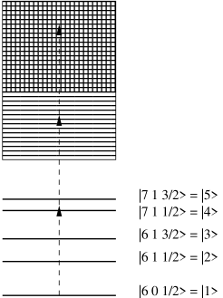
Figure 1: Energy level structure for the Cesium five level system, with the excited states coupled to a continuum of states

Figure 2: Ionization channels from the ground state of cesium

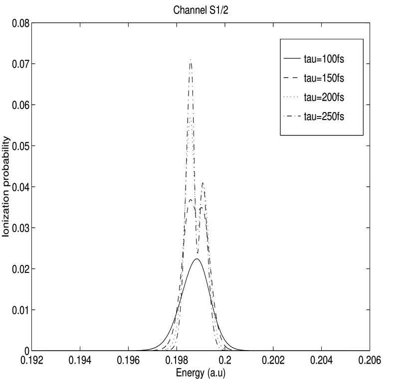
Figure 3: Probability per unit energy vs. energy for the photoelectron produced by a two photon ionization of cesium for various pulse lengths. Laser frequency 0.0994 a.u., peak intensity $10^{-7}$a.u. ($1.4\times 10^{10}\rm{W/cm}^{2}$), no chirping.

Figure 4: Probability per unit energy vs. energy for the photoelectron produced by a two photon ionization of cesium. The solid line is the spectrum for the S_1/2 channel, the other curves represent the contribution of ionization from the 7p levels separately (no interference effects). Laser frequency 0.0994 a.u., peak intensity $10^{-7}$a.u. ($1.4\times 10^{10}\rm{W/cm}^{2}$), pulse length 250fs, no chirping.

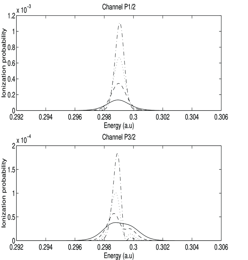
Figure 5: Probability per unit energy vs. energy for the photoelectron produced by a two photon ionization of cesium for various pulse lengths. Laser frequency 0.0997 a.u., peak intensity $10^{-7}$ a.u. ($1.4\times 10^{10}\rm{W/cm}^{2}$), no chirping; pulse length $\tau$ is $-$ 100 fs,$--$ 150 fs, $\cdot\cdot$ 200 fs,$\cdot-$ 250 fs.

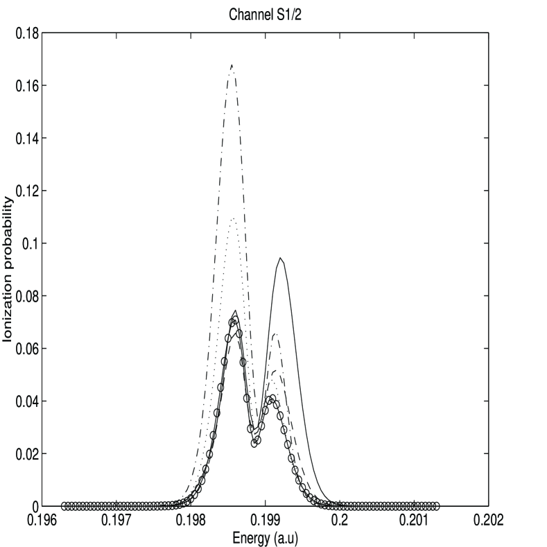
Figure 6: Probability per unit energy vs. energy for the photoelectron produced by a two photon ionization of cesium for different chirping parameters. The final continuum state is an S_1/2 channel. Laser frequency 0.0994 a.u., pulse length 250 fs, peak intensity $10^{-7}$ a.u. ($1.4\times 10^{10}\rm{W/cm}^{2}$), line type correspond to different chirp parameters $\beta$: $-$ -0.0003 a.u., $--$ -0.0002 a.u., o 0.0 a.u., $\cdot\cdot$ 0.0002 a.u., $-\cdot$ 0.0003 a.u.

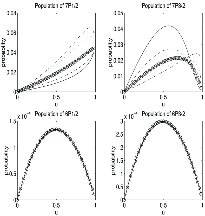
Figure 7: Populations of the 7p levels vs compressed time for different chirp parameters. Laser frequency 0.0994 a.u., pulse length 250 fs, peak intensity $10^{-7}$ a.u. ($1.4\times 10^{10}\rm{W/cm}^{2}$), line type correspond to different chirp parameters $\beta$: $-$ -0.0003 a.u., $--$ -0.0002 a.u., o 0.0 a.u., $\cdot\cdot$ 0.0002 a.u., $-\cdot$ 0.0003 a.u.

Figure 8: Probability per unit energy vs. energy for the photoelectron produced by a two photon ionization of cesium for various intensities. The final continuum state is an D_3/2 channel. The laser is tuned outside the 7p doublet, at the frequency 0.099 a.u., the pulse length is 25 fs. The peak intensity in the legend is given in atomic units.

Figure 9: Population of the 7p levels vs compressed time, for various intensities. The parameters are the same as in fig. 8

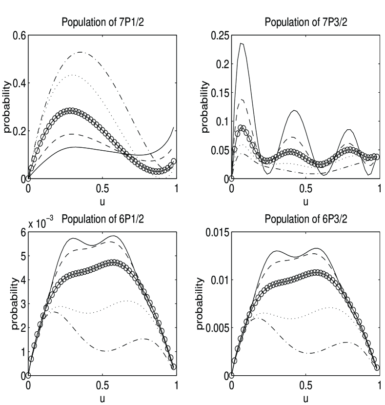
Figure 10: Populations of the 7p levels vs compressed time for different chirp parameters. Laser frequency 0.0994 a.u., pulse length 250 fs, peak intensity $0.7\times 10^{-5}$a.u., line type correspond to different chirp parameters $\beta$: $-$ -0.0003 a.u., $--$ -0.0002 a.u., o 0.0 a.u., $\cdot\cdot$ 0.0002 a.u., $-\cdot$ 0.0003 a.u.

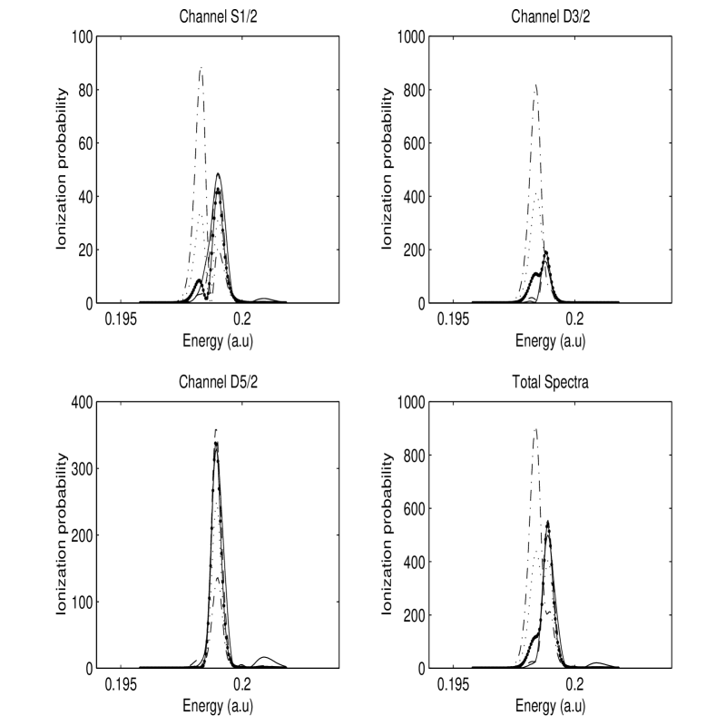
Figure 11: Probability per unit energy vs. energy for the photoelectron produced by a two photon ionization of cesium for different chirping parameters. The final continuum states are the S_1/2, D_3/2 and D_5/2 channels and the total probability for 2 photon ionization. Laser frequency 0.0994 a.u., pulse length 250 fs, peak intensity $0.7\times 10^{-5}$ a.u., line type correspond to different chirp parameters $\beta$: $-$ -0.0003 a.u., $--$ -0.0002 a.u., solid/dotted line 0.0 a.u., $\cdot\cdot$ 0.0002 a.u., $-\cdot$ 0.0003 a.u.

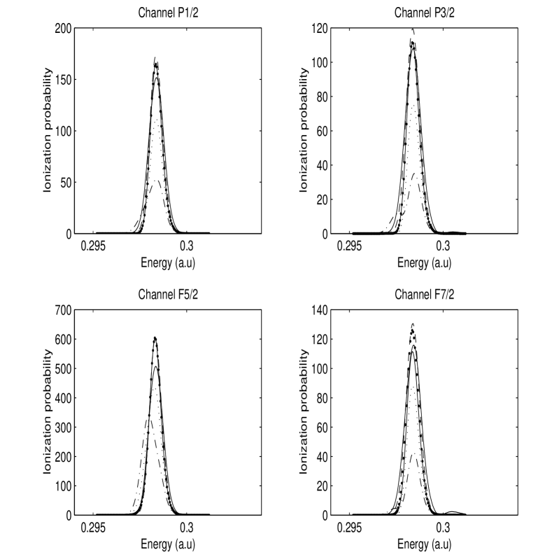
Figure 12: Probability per unit energy vs. energy for the photoelectron produced by a three photon ionization of cesium for different chirping parameters. Laser frequency 0.0994 a.u., pulse length 250 fs, peak intensity $0.7\times 10^{-5}$ a.u., line type correspond to different chirp paprameters $\beta$: $-$ -0.0003 a.u., $--$ -0.0002 a.u., solid/dotted line 0 a.u., $\cdot\cdot$ 0.0002 a.u., $-\cdot$ 0.0003 a.u.

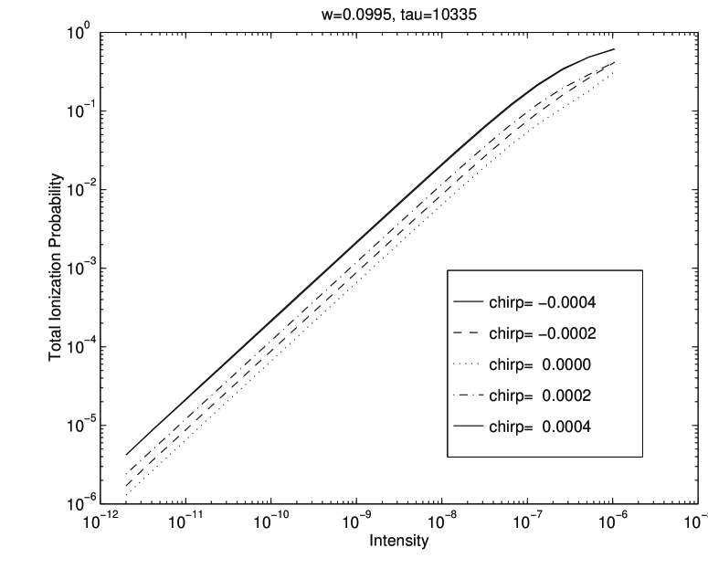
Figure 13: Total ionization probability as a function of intensity for different chirpings (in a.u.). The laser frequency is 0.0995 a.u. and the pulse length 250fs.

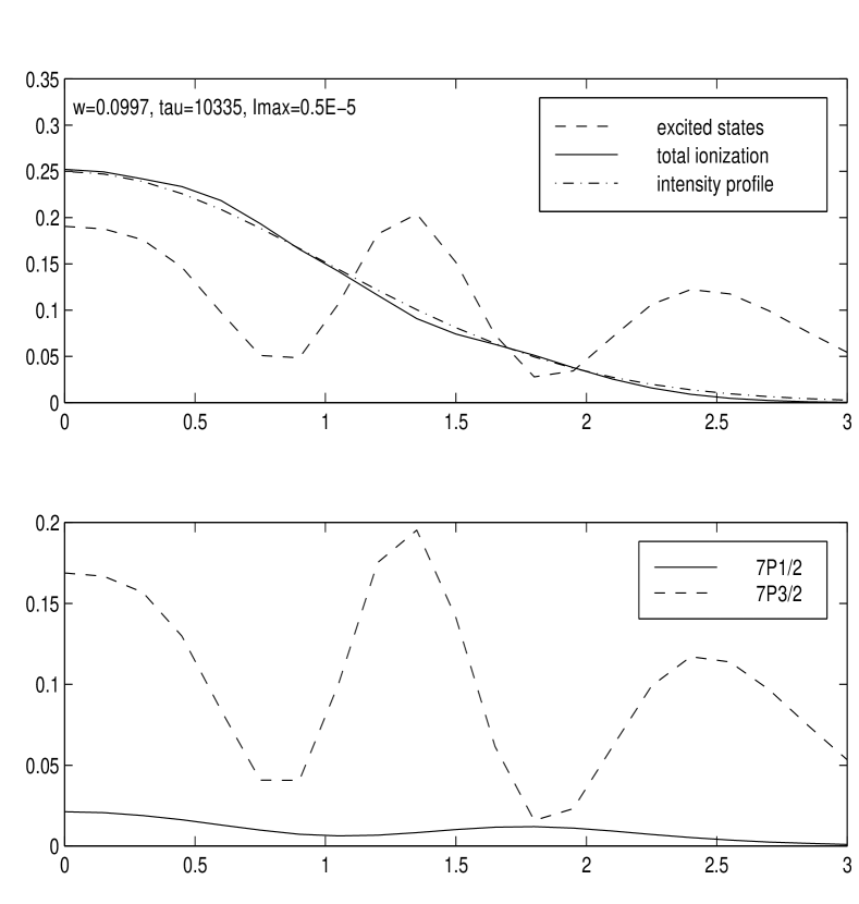
Figure 14: Residual total population of the excited states and total ionization probability vs. distance r from the axis of a Gaussian laser beam. The Gaussian beam profile is shown for reference (dash–dotted line). Laser frequency 0.0997 a.u., pulse length 250 fs, peak intensity 0.7$\times 10^{12}$ W/cm², no chirping.

Figure 15: Population vs. compressed time u and distance r from the axis of a Gaussian laser beam. Laser frequency 0.0993 a.u., pulse length 250 fs, peak intensity 0.7$\times 10^{12}$ W/cm², no chirping.

Figure 16: Probability per unit energy vs. energy for the photoelectron produced by a two photon ionization of cesium vs. energy Ef and distance r from the axis of a Gaussian laser beam. Laser frequency 0.0993 a.u., pulse length 250 fs, peak intensity 0.7$\times 10^{12}$ W/cm², no chirping.

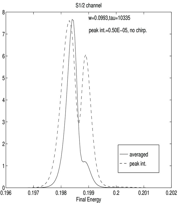
Figure 17: Probability per unit energy for the photoelectron produced by a two photon ionization of cesium vs. energy Ef. The final continuum states are the S_1/2 Laser frequency 0.0993 a.u., peak intensity 0.7 $\times 10^{12}$ W/cm², pulse length 250 fs, no chirping. Space averaged spectra (continuous line) and peak intensity spectra (dashed line).

References

- [1] N. B. Delone and V. P. Krainov, Atoms in Strong Light Fields, Vol. 28 of Springer series in chemical physics (Springer-Verlag, New York, 1984).
- [2] R. M. Potvliege and R. Shakeshaft, Phys. Rev. A 41, 1609 (1990).
- [3] M. Dörr et al., J. Phys. B 25, 2809 (1992).
- [4] H. R. Reiss, Phys. Rev. A 22, 1786 (1980).
- [5] H. R. Reiss, Phys. Rev. A 42, 1476 (1990).
- [6] G. Petite, P. Agostini, and H. G. Muller, J. Phys. B 21, 4097 (1988).
- [7] J. H. Eberly, J. Javanainen, and K. Rzazewski, Phys. Rep. 204, 331 (1991).
- [8] J. Javanainen, J. H. Eberly, and Q. Su, Phys. Rev. A 38, 3430 (1988).
- [9] S. Geltman, J. Phys. B 27, 1497 (1994).
- [10] K. C. Kulander, Phys. Rev. A 38, 778 (1988).
- [11] N. Rosen and C. Zener, Phys. Rev 40, 502 (1932).
- [12] R. T. Robiscoe, Phys. Rev. A 17, 247 (1978).
- [13] A. Adler, A. Rachman, and E. J. Robinson, J. Phys. B 28, 5057 (1995).
- [14] A. Burgess and M. J. Seaton, Mon. Not. R. Astron. Soc. 120, 121 (1960).
- [15] P. Stone, Phys. Rev. 127, 1161 (1962).
- [16] F. Herman and S. Skillman, Atomic Structure Calculations (Prentice Hall, Englewood Cliffs, NJ, 1963).
- [17] P. Lambropoulos and M. R. Teague, J. Phys. B 9, 587 (1976).
- [18] S. E. Koonin and D. C. Meredith, Computational Physics (Addison–Wesley, New York, 1990).
- [19] M. Abramowitz and I. A. Stegun, Handbook of Mathematical Functions with formulas, graphs, and mathematical tables (U.S. Govt. Print. Off., Washington, D.C., 1994).
- [20] Compact Sources of Ultrashort Pulses, Cambridge Series in Modern Optics, edited by I. N. I. Duling (Cambridge University Press, Great Britain, 1995).
- [21] M. T. Asaki et al., Opt. Lett. 18, 977 (1993).
- [22] W. Nicklich et al., Phys. Rev. Lett. 69, 3455 (1992).
- [23] A. Adler, A. Rachman, and E. J. Robinson, J. Phys. B 28, 5077 (1995).
- [24] M. Edwards and C. W. Clark, J. Opt. Soc. Am. B 13, 101 (1996).