One class of integrals evaluation in magnet solitons theory

Abstract

An analytical-numeric calculation method of extremely complicated integrals is presented. These integrals appear often in magnet soliton theory.

The appropriate analytical continuation and a corresponding integration contour allow to reduce the calculation of wide class of integrals to a numeric search of integrand denominator roots (in a complex plane) and a subsequent residue calculations. The acceleration of series convergence of residue sum allows to reach the high relative accuracy limited only by roundoff error in case when $10\div 15$ terms are taken into account.

The circumscribed algorithm is realized in the C program and tested on the example allowing analytical solution. The program was also used to calculate some typical integrals that can not be expressed through elementary functions. In this case the control of calculation accuracy was made by means of one-dimensional numerical integration procedure.

1 Introduction

Nonlinear excitations (topological solitons [1]) play an important role in the physics of low-dimensional magnets [2, 3]. They contribute greatly to a heat capacity, susceptibility, scattering cross-section and other physical characteristics of magnets. In particular, for two-dimensional (2D) magnets with discrete degeneracy it is important to take into account the localized stable (with quite-long life time) 2D solitons [2, 3]. According to the experiments [4], these solitons determine the relaxation of magnetic disturbance and can produce peaks in the response functions.

The traditional model describes the magnet state in terms of the unit magnetization vector $\vec{m}$, $\vec{m}^{2}=1$ with the energy function in the form

$$W=\int\limits d^{2}x\left\{A(\nabla\vec{m})^{2}+w_{0}(\vec{m})\right\},$$ (1)

where A is the nonuniform exchange constant and $w_{0}(\vec{m})$ - the anisotropy energy.

In an anisotropic case the solution is multi-dimensional, that is why the soliton structure is determined by the system of equations in partial derivatives. There are no general methods of finding the localized solutions to such equations and analyzing the stability of the solution. For this reason a direct variational method is often used. Consequently, a choice of a trial function plays a key role in such analysis [5, 6, 7]. In most cases a quite successful choice of trial function is as follows:

$$tg{\theta\over 2}={R\over r}\exp\left(-\frac{r}{a}\right)(1+C_{1}\cos 2\chi),\qquad\varphi=\chi+C_{2}\sin 2\chi+\varphi_{0},$$ (2)

where $r$, $\chi$ are the polar coordinates in a magnetic plane, $R$, $a$, $C_{1}$, $C_{2}$ and $\varphi_{0}$ - variated parameters.

In papers [5, 6, 7] the iterative Newton method of solving the non-linear system of algebraic equations [8] was used to find the variated parameters providing an energy minimum. The numerical algorithm mentioned above results in the necessity of multiple calculation of two-dimensional integrals (by the angle $\chi$ and radius $r$). Experience reveals that the calculation process could be essentially accelerated (and the calculation precision improved) if the analytical-numeric procedure for the integrals by radius are made beforehand. The typical form of these integrals is:

$$\int\limits_{0}^{\infty}{f(r)\exp(mr)dr\over\left[(r\exp(r))^{2}+a^{2}\right]^{n}}$$ (3)

where $n,m$ - integer numbers ($m<2n$), $f(r)$ - polynomial of degree $k$ in variable $r$. It is convenient to denote $g(r)\equiv f(r)\exp(mr)$. Possible expressions for $g(r)$ are $r\exp(r)$, $(1+r)\exp(r)$, $r^{2}\exp(r)$ and so on. Note, that $a$ is essential parameter - no substitution exists to eliminate it. Below we shall consider the case $n=1$. From the one hand it is, practically, always possible to reduce the calculation at $n>1$ to a sum of integrals at $n=1$. From the other hand it is not difficult to modify evaluation scheme if $n>1$.

Further we show that the indicated type of integrals may be calculated both analytically and numerically (by the use of joint analytical and numerical methods). To obtain the desired accuracy one should find integrand residues (numerically) and build approximate expression (see below).

Main analytical expressions that allow to find integrals like (3) are presented in Analytical Formulae and the C version of corresponding program is given in Program Realization.

The theory of function of a complex variable gives the powerful method of definite integrals calculation. In the considered case the algorithm realization is quite problematical because the expressions for the roots in a complex plane could not be written analytically. Correspondingly, one can not write down and analytically summarize expressions for residues.

Present paper pays attention to the fact that numerical methods (roots search in complex plane and calculation of residue sum) together with analytical ones allow to use the theory of complex variable with the same efficiency like in the traditional consideration.

2 Analytical formulae

The usual way of integral (3) evaluation is to continue analytically the integrand function in some complex domain $D$. In this case the evaluating integral will be the part of the integral over the closed contour $C$ in a complex plane. This contour comprises the real axis interval and the arc $S$ closing the integration contour. So, the solution of the problem can be readily obtained if integral value over arc $S$ tends to the zero. The integral value over contour $C$ can be calculated with a help of the Residue Theorem. In some cases the evaluating integral will be the real or imaginary part of a contour integral.

Let’s consider the function of a complex variable

$$F(z)={g(z)ln(z)\over\ (z\exp(z))^{2}+a^{2}},$$ (4)

For this integrand function the conditions of Cauchy’s theorem and Jordan’s lemma are fulfilled. So the integral along the arc of infinite radius is vanishing and $g(z)$ have no branch point. Note that all the examples above meet these conditions.

2.1 Integration contour

Since $\ln(z)$ is a multiple-valued function, it is necessary to use the cut plane. Usual method (see, for example [9]) of dealing with integrals of this type is to use a contour large circle $C_{\infty}$, center the origin, and radius $R$; but we must cut the plane along the real axis from $0$ to $\infty$ and also enclose the branch point $z=0$ in a small circle $c_{0}$ of radius $r$. The contour is illustrated in Fig 1.

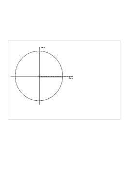
Figure 1: Integration contour

Evidently, we may write down the Cauchy’s theorem in a form:

$$\int\limits_{0}^{\infty}{g(x)\ln(x)dx\over(x\exp(x))^{2}+a^{2}}+\int\limits_{C_{\infty}}{g(z)\ln(z)dz\over(z\exp(z))^{2}+a^{2}}+\int\limits^{0}_{\infty}{g(x)(\ln(x)+2\pi i)dx\over(x\exp(x))^{2}+a^{2}}$$

$$+\int\limits_{c_{0}}{g(z)\ln(z)dz\over(z\exp(z))^{2}+a^{2}}=2\pi i\sum\limits_{k=0}^{\infty}resF(z_{k}),$$ (5)

where $C_{\infty}$ is an arc of infinitely great radius, $c_{0}$ - an arc of an infinitesimally one. Integrals over these circles are vanishing. Also taking into account the cancellation of integrals evaluated in opposite directions we obtain:

$$\int\limits_{0}^{\infty}{g(x)dx\over(x\exp(x))^{2}+a^{2}}=-\sum\limits_{k=0}^{\infty}resF(z_{k}).$$ (6)

Thus the evaluating integral is equal to a sum of integrand residues inside the contour. The direct calculation of the residue sum in integrand poles leads to extremely slow convergence of the partial sums. Nevertheless, we shall see below that the convergence series acceleration (Euler’s transformation [12]) allows to take at most $10\div 15$ terms into account.

Following the obvious method one must search the denominator roots and substitute the evaluated residues in series (6).

2.2 Denominator zeros

The denominator zeros are roots of two equations:

$$z\exp(z)-ia=0,\quad\mbox{and}\quad z\exp(z)+ia=0.$$ (7)

Further we will consider only the first equation of (7) as the solution of the second one is complex conjugate to the first one. Separating real ($x=Rez$) and imaginary ($y=Jmz$) parts of equation (7) leads to a set (system) of two nonlinear equations:

$$x\cos y-y\sin y=0,\qquad y\cos y+x\sin y-a\exp(-x)=0.$$ (8)

Simple algebraic transformations allow to reduce this system to:

$$\sin y={x\exp(x)\over a},\qquad x\cos y-y\sin y=0$$ (9)

As it will be shown below some roots of equation (7) have the positive real part ($x>0$). Nevertheless, in this case the magnitude $x\exp(x)/a$ does not exceed unit. For the roots with negative real part ($x<0$) at $a>1/e$ always $|x\exp(x)/a|<1$. At $a<1/e$ there exists a region of negative $x$ values where $x\exp(x)/a<-1$. But it’s easy to show that no roots of (7) meet this region.

Let’s write down the solution of the first equation (9) in a form:

$$y=(-1)^{N}\arcsin{x\exp(x)\over a}+N\pi,\qquad N=0,\pm 1,\pm 2,\pm 3,\ldots.$$ (10)

Integer number $N$ separate different branches of function $\mathop{\rm arctg}\nolimits$. The $y$ value for these branches lie in the limits:

$$(2N-1)\frac{\pi}{2}\leq y\leq(2N+1)\frac{\pi}{2},\quad N=0,\pm 1,\pm 2,\pm 3,\ldots.$$ (11)

After substitution expression (10) into the second equation of the system (8), we obtain:

$$(-1)^{N}\arcsin{x\exp(x)\over a}+N\pi=\pm a\exp(-x)\sqrt{1-\left({x\exp(x)\over a}\right)^{2}}.$$ (12)

If $N=\pm 2m$ ($m=0,1,2,\ldots$) $\cos y>0$ and we chose the upper sign (plus) in the right-hand side of equation (12). Contrary to this, $\cos y<0$ if $N=\pm(2m+1)$ and we must chose the lower sign (minus) in the right-hand side of equation (12). Thus at even $N$ ($N=\pm 2m$) we obtain:

$$\arcsin{x\exp(x)\over a}+N\pi=a\exp(-x)\sqrt{1-\left({x\exp(x)\over a}\right)^{2}},$$ (13)

and at odd $N$ ($N=\pm(2m+1)$) respectively:

$$\arcsin{x\exp(x)\over a}-N\pi=a\exp(-x)\sqrt{1-\left({x\exp(x)\over a}\right)^{2}}.$$ (14)

It is easy to see, that equation (13) have solutions only at $N\geq 0$, while (14) one only at $N<0$. Therefore, it is convenient to unite (13) and (14) and write down:

$$\arcsin{x\exp(x)\over a}+k\pi-a\exp(-x)\sqrt{1-\left({x\exp(x)\over a}\right)^{2}}=0,\quad k=0,1,2,\ldots$$ (15)

The point to keep in mind, that $\cos y>0$ at $k=2m$ and $\cos y<0$ at $k=2m+1$. At even $k=2m$ and $x<0$ it is not difficult to build an approximation for the real and imaginary parts of the root $z_{k}$:

$$x_{k}\approx-\left[1+{\ln{k\pi/a}\over 2(k\pi)^{2}}\right]\ln{k\pi\over a},\qquad y_{k}\approx k\pi.$$ (16)

As $x<0$ and $y>0$ the argument of the complex number is placed in the second quarter (less than $\pi$, but greater than $\pi/2$) and is equal to:

$$\arg z_{k}\approx{\pi\over 2}+\mathop{\rm arctg}\nolimits{k\pi\over\ln(k\pi/a)}.$$ (17)

Just note that complex conjugate number argument is placed in the third quadrant ($x<0$ and $y<0$) and:

$$\arg\overline{z}_{k}\approx{3\pi\over 2}-\mathop{\rm arctg}\nolimits{k\pi\over\ln(k\pi/a)}.$$ (18)

The comparison of these solutions with exact numerical one will be given below in Table 1.

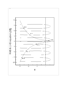
Figure 2: Denominator zeroes in complex plane

At odd $k=2m+1>0$ the argument of the root and complex conjugate value are equal respectively:

$$\arg z_{k}\approx{3\pi\over 2}-\mathop{\rm arctg}\nolimits{k\pi\over\ln(k\pi/a)}$$

$$\arg\overline{z}_{k}\approx{\pi\over 2}+\mathop{\rm arctg}\nolimits{k\pi\over\ln(k\pi/a)}.$$ (19)

The comparison of these solutions with exact numerical one will also be given in Table 1.

Hence, evaluation of the complex roots of equation (7) is reduced to a real part $z_{k}$ search (transcendental equation (15) solution) and further calculation of imaginary part $z_{k}$ by (10). The graphs of the sum of the first two terms of (15) and the third term of the equation (15) are presented on Fig 2.

Intersection points of these curves marked by circles correspond to the roots of equation (15). Any of the roots marked on Fig 2. can be evaluated numerically with the help of Newton-Rafson method (e.g. [10]). The approximations (16) are used as an initial guess. Necessary explanation will be made in the Program Realization. It is convenient to number these roots by corresponding values of $k$ as it is shown on the figure (the numeration is used in the program).

Table 1: Relative error between exact value and approximation
for different $a$

k	a=1/e	a=1.0	a=10
$1$	$9.21835\cdot 10^{-2}$	$1.11473\cdot 10^{-1}$
$2$	$2.40163\cdot 10^{-2}$	$2.52883\cdot 10^{-2}$
$3$	$1.09204\cdot 10^{-2}$	$1.11533\cdot 10^{-2}$
$4$	$6.21187\cdot 10^{-3}$	$6.27698\cdot 10^{-3}$	$6.35174\cdot 10^{-3}$
$5$	$4.00030\cdot 10^{-3}$	$4.02305\cdot 10^{-3}$	$4.06565\cdot 10^{-3}$
$6$	$2.78844\cdot 10^{-3}$	$2.79747\cdot 10^{-3}$	$2.82172\cdot 10^{-3}$
$7$	$2.05364\cdot 10^{-3}$	$2.05747\cdot 10^{-3}$	$2.07187\cdot 10^{-3}$
$8$	$1.57493\cdot 10^{-3}$	$1.57657\cdot 10^{-3}$	$1.58551\cdot 10^{-3}$
$9$	$1.24585\cdot 10^{-3}$	$1.24651\cdot 10^{-3}$	$1.25229\cdot 10^{-3}$
$10$	$1.01001\cdot 10^{-3}$	$1.01021\cdot 10^{-3}$	$1.01407\cdot 10^{-3}$

In case $Rez>0$ (it will be if $a>|k\pi|$) it is more convenient to find roots by bisection because it is difficult to get a necessary initial guess. At the same time it is obvious from Fig 2 that at $Rez>0$ each subsequent root lies between zero and a root found before.

2.3 Residue Calculation

2.3.1 The test integral

Let’s consider the test example of an integral (3) when $m=1$ and $g(r)=(1+r)\exp(r)$. Elementary analytic calculation yields $\frac{1}{2}\pi/a$. On the other hand function $F(z)$ residue in the pole of first order (at the same $g(x)$) is equal:

$$resF(z_{k})=\left.{(1+z)\exp(z)\ln(z)\over{\displaystyle{d\over dz}}[(z\exp(z))^{2}+a^{2}]}\right|_{z_{k}}=\left.{\ln(z)\over 2z\exp(z)}\right|_{z_{k}}=\left.\mp{i\ln(z)\over 2a}\right|_{z_{k}},$$ (20)

where upper sign (minus) corresponds to the first and lower (plus) to the second of the equations (7).

Let’s take the equation (6) in a form:

$$\int\limits_{0}^{\infty}{(1+x)\exp(x)dx\over(x\exp(x))^{2}+a^{2}}=-\sum\limits_{k=0}^{\infty}resF(z_{k})={i\over 2a}\sum\limits_{k=0}[\ln(z_{k})-\ln(\overline{z}_{k})]$$

$$={i\over 2a}\sum\limits_{k=0}[i\arg(z_{k})-i\arg(\overline{z}_{k})]={1\over 2a}\sum\limits_{k=0}[\arg(\overline{z}_{k})-\arg(z_{k})].$$ (21)

For the following evaluation it is important to determine root arguments correctly. Here and below in this article the complex value argument will be determined by principal value of $\mathop{\rm arctg}\nolimits$ in order to use the library function $\mathop{\rm arctg}\nolimits$ within the limits of first quadrant. The point to keep in mind is that the quadrant of the complex value one have to define ”by hand”. It allows to avoid mistakes connected with possible definitions of library functions of negative argument, etc.

Let’s consider first three terms of the series summarized:

1. If $k=0$ the root $z_{0}$ is placed in the first quadrant and its’ argument is equal to $\varphi_{0}=\mathop{\rm arctg}\nolimits|y_{0}/x_{0}|$. Evidently, that the complex conjugate value has the argument $2\pi-\varphi_{0}$. Contribution of these two poles in the right-hand side of equation (21) is:

   $$\arg(\overline{z}_{0})-\arg(z_{0})=2\pi-2\varphi_{0}$$

2. The next root $z_{1}$ (at $k=1$) is placed in the third quadrant and its’ argument is equal to $\pi+\varphi_{1}=\pi+\mathop{\rm arctg}\nolimits|y_{1}/x_{1}|$. Complex conjugate value argument is $\pi-\varphi_{1}=\pi-\mathop{\rm arctg}\nolimits|y_{1}/x_{1}|$. Corresponding contribution of these roots is:

   $$\arg(\overline{z}_{1})-\arg(z_{1})=-2\varphi_{1}$$

3. Consider one root more at $K=2$. Its’ argument is equal to $\pi-\varphi_{2}=\pi-\mathop{\rm arctg}\nolimits|y_{2}/x_{2}|$. For the complex conjugate value we obtain $\pi+\varphi_{2}=\pi+\mathop{\rm arctg}\nolimits|y_{2}/x_{2}|$. Thus, we find:

   $$\arg(\overline{z}_{2})-\arg(z_{2})=2\varphi_{2}$$

Structure of each term is clear that is why we simply quote the result:

$$\int\limits_{0}^{\infty}{(1+x)\exp(x)dx\over(x\exp(x))^{2}+a^{2}}={1\over 2a}\sum\limits_{k=0}[\arg(\overline{z}_{k})-\arg(z_{k})]=$$ (22)

$$= {1\over 2a}\left[2\pi-2\varphi_{0}-2\varphi_{1}+2\varphi_{2}-2\varphi_{3}+2\varphi_{4}-\ldots\right]$$

$$= {1\over a}\left[\pi-\left(\varphi_{0}+\varphi_{1}-\varphi_{2}+\varphi_{3}-\varphi_{4}+\ldots\right)\right]$$

The sum $\varphi_{k}$ is found numerically. This series is conventional convergent. Partial sums consecutively equal to $\simeq 0.81$ and $\simeq 2.3$ and converge very slowly. Nevertheless, the program of convergence acceleration [8] found the result $\pi/2$ with the relative error that does not exceed $10^{-8}$ ($10\div 15$ terms of the series are taken into account).

2.3.2 First order pole

In this section we will consider integral (3) at $m=1$ and $g(r)=\exp(r)$. The residue of integrand function $F(z)$ in the first order pole is evidently equal to:

$$resF(z_{k})=\left.{\exp(z)\ln(z)\over{\displaystyle{d\over dz}}[(z\exp(z))^{2}+a^{2}]}\right|_{z_{k}}=\left.{\ln(z)\over 2z\exp(z)(1+z)}\right|_{z_{k}}=\left.\pm{i\ln(z)\over 2a(1+z)}\right|_{z_{k}}.$$ (23)

As in the previous case the upper sign (minus) corresponds to the first and lower (plus) to the second of the equations (7).

It is convenient to write down residue expression in a form:

$$\int\limits_{0}^{\infty}{\exp(x)dx\over(x\exp(x))^{2}+a^{2}}=-\sum\limits_{k=0}^{\infty}resF(z_{k})={i\over 2a}\sum\limits_{k=0}\left[{\ln(z_{k})\over 1+z_{k}}-{\ln(\overline{z}_{k})\over 1+\overline{z}_{k}}\right]$$

$$={i\over 2a}\sum\limits_{k=0}\left[{\ln|z_{k}|+i\arg(z_{k})\over 1+z_{k}}-{\ln|\overline{z}_{k}|+i\arg(\overline{z}_{k})\over 1+\overline{z}_{k}}\right].$$ (24)

The argument value depends on denominator zeros placement. Obviously, there are four possibilities.

For the complex roots lying in the first quadrant (it will be if $k=0,2,4\ldots$, at $a>k\pi$) the first term in (24) is equal to:

$${\ln|z_{0}|+i\varphi_{0}\over 1+z_{0}}$$

Second term (for the complex conjugate value) yields:

$${\ln|\overline{z}_{0}|+i(2\pi-\varphi_{0})\over 1+\overline{z}_{0}}$$

Subtracting the terms and separating real and imaginary parts (factor $i/2a$ is taken into account) we obtain:

$${y_{0}\ln|z_{0}|+(1+x_{0})(\pi-\varphi_{0})\over a|1+z_{0}|^{2}}+i{\pi y_{0}\over a|1+z_{0}|^{2}}$$ (25)

Pay attention that the angle $\varphi_{0}$ is determined as the principal value of $\mathop{\rm arctg}\nolimits$ in the limits $[0,\pi/2]$.

Similary calculations for the second, third and fourth quadrants give respectively:

$${y_{2}\ln|z_{2}|+(1+x_{2})\varphi_{2}\over a|1+z_{2}|^{2}}+i{\pi y_{2}\over a|1+z_{2}|^{2}},$$ (26)

$${y_{3}\ln|z_{3}|-(1+x_{3})\varphi_{3}\over a|1+z_{3}|^{2}}+i{\pi y_{3}\over a|1+z_{3}|^{2}},$$ (27)

$${y_{1}\ln|z_{1}|-(1+x_{1})(\pi-\varphi_{1})\over a|1+z_{1}|^{2}}+i{\pi y_{1}\over a|1+z_{1}|^{2}},$$ (28)

As if structure of each term is already clear then it is not hard to write the sum of real residue parts (25-28) and all the subsequent ones.

$$\int\limits_{0}^{\infty}{\exp(x)dx\over(x\exp(x))^{2}+a^{2}}=-\sum\limits_{k=0}^{\infty}res(F(z_{k}))$$ (29)

$$= \frac{1}{a}\left[{y_{0}\ln|z_{0}|+(1+x_{0})(\pi-\varphi_{0})\over|1+z_{0}|^{2}}+{y_{1}\ln|z_{1}|-(1+x_{1})\varphi_{1}\over|1+z_{1}|^{2}}\right.$$

$$+ {y_{2}\ln|z_{2}|+(1+x_{2})\varphi_{2}\over|1+z_{2}|^{2}}+{y_{3}\ln|z_{3}|-(1+x_{3})\varphi_{3}\over|1+z_{3}|^{2}}$$

$$+ \left.{y_{4}\ln|z_{4}|+(1+x_{4})\varphi_{4}\over|1+z_{4}|^{2}}+\ldots\right]$$

Sum of not more than 15 terms of this series give right result for any $a>0.0006$ if acceleration of series convergence is used. The partial sums of the imaginary parts also rapidly ($\sim 10\div 15$ terms) tends to the zero ($\sim 10^{-12}$).

2.4 Approximation at $a$ vanishing

At $a$ vanishing it is convenient to write down the approximate expression for integral (24). Let’s set $m=1$ in (3) and make substitution:

$$x\exp(x)=au,$$ (30)

where $u$ is the new independent variable. Left-hand side of equation (30) may be expanded in powers of the x:

$$au\approx x+x^{2}+\frac{1}{2!}x^{3}+\ldots$$ (31)

Inversion [12] of this series gives:

$$x\approx au-(au)^{2}+\frac{3}{2}(au)^{3}-\ldots$$ (32)

For the present purposes, it is sufficient to retain only one term in right-hand side of equation (32). We will focus on the case discussed in the previous section, namely, $f(x)=\exp(x)$. Simple integration leads to the following result:

$$\int\limits_{0}^{\infty}{\exp(x)dx\over(x\exp(x))^{2}+a^{2}}\approx\frac{1}{a(1+a^{2})}\left[\frac{\pi}{2}+a\ln(a)\right]$$ (33)

One more term taking into account yields:

$$\int\limits_{0}^{\infty}{\exp(x)dx\over(x\exp(x))^{2}+a^{2}}$$ (34)

$$\approx \frac{1}{(1+a^{2})^{2}+a^{2}}\left\{(1+a^{2})\frac{\pi}{2a}+\ln(a)+{3+2a^{2}\over 2\sqrt{5}}\ln\left|{1+\sqrt{5}\over\sqrt{5}-1}\right|\right\}$$

Quality of these approximations is presented in Table LABEL:tab:number2.

As one can see the relative error given by approximation (34) is not worth than $2.62\cdot 10^{-5}$ at $a=6\cdot 10^{-4}$ and smaller for other values. If it is necessary, the approximation (34) can be improved.

3 Program Realization

Program text consists of the principal routine (main) and eight procedures:

• Root - subroutine for searching real part of denominator zeros. Newton-Rafson iteration method used for this purpose.

• Fun - subroutine for left-hand side equation (15) evaluation.

• Der - subroutine for left-hand side of equation (15) derivative evaluating.

• Approximation - evaluate initial guess to the root according to the (16).

• Eulsum - program of acceleration of series (29) convergence. The C version of corresponding FORTRAN program [8] is used.

• Bisection - recursive version of bisection root finding.

• Right_bound - auxiliary program. Determine the right bound of root region.

• Sign - auxiliary program for Bisection. Determine sign of variable $x$.

The demonstration version of the program is presented below. The first four statements declare the necessary functions that are used in the program.

#include <dos.h>
#include <stdio.h>
#include <math.h>
#include <alloc.h>

// Declaration of functions used below.

double Fun(double);
double Der(double);
double Bisection(double& ,double& ,double& ,double&);
double Root(double);
double Approximation_x(void);
double Right_bound(void);
void Eulsum(double&, double, int);
int Sign(double);

// // //

Defining of the global constants. Parameter $A\equiv a$ can be defined in any other way. EPS - relative accuracy for root search; K - root number; N - number of roots taking into account.

double  A = 0.2, EPS = 1.0e-14;
long unsigned irec = 0, irecmax = 100;
int K, N = 20;

// // //

Definition of parameters used by procedures Root (x, y, yx, phi_k, den, argument) and Bisection (a, c, funa, func, xold, xk). See below.

void main(void)
{ double x, y, yx, phi_k, den, argument;
  double real_part = 0, imag_part = 0;
  double a, c, funa, func, xold, xk;
  double *real_term = (double*)calloc(N,sizeof(double));
  double *imag_term = (double*)calloc(N,sizeof(double));

// //

Two previous statements reserved memory for storaging denominator roots. Cycle on root numbers begins below.

  xold = 0.99999*Right_bound();
  for(int k = 0; k < N; k++)
  { K = (k%2) ? -k : k;

// // //

Variable $K$ (upper case) takes values $0,-1,2-3,\ldots$ while $k=0,1,2,3,\ldots$. Statements IF ELSE differs three different cases: $Real(z_{k})=0$, $Real(z_{k})>0$ and $Real(z_{k})<0$.

    if(A == fabs(K*M_PI)) x = 0.0;
    else { if(A > fabs(K*M_PI))
              { a = 0.0; c = xold;
                funa = Fun(a);   func = Fun(c);
                x = Bisection(a,c,funa,func);
                xold = 0.99999999 * x;  irec = 0;}
            else
              { xk = Approximation_x();
                x = Root(xk);                 }
          }

// //

The following statements calculate argument of $z_{k}$ and store real and imaginary parts of the term to be summarized.

y = pow(-1,k)*asin(x*exp(x)/A) + K*M_PI;

if(x == 0) argument = M_PI_2;

else { yx = fabs(y/x);

phi_k = atan(yx);

argument = (x > 0) ? M_PI - phi_k : phi_k;}

den = (1+x)*(1+x)+y*y;

real_term[k]=(0.5*y*log(x*x+y*y)+(1+x)* Sign(y)*argument)/den;

imag_term[k]=y/den;

}

// // // //

End cycle on root numbers. Accelerating the rate of a sequence of partial sums performed by the procedure Eulsum. This is the $C$ version of Van Wijngaarden’s algorithm (see [8]). Then the result is printed. The last two statements free the allocated memory.

  for(int j = 0; j < N; j++) Eulsum(real_part,real_term[j],j);
  for(    j = 0; j < N; j++) Eulsum(imag_part,imag_term[j],j);
  printf("Real part =%12.5lf ",real_part/A);
  printf("Imaginary part =%12.5le \n",imag_part);
  free(real_term);
  free(imag_term);
}

// //

Initial guess for the Newton-Rafson iteration is chosen with respect to parameter $a$ value. The appointments of other statements are evident.

double Root(double xk)
{ double xk1;
  for(int it = 0; it < 30; it++)
   { xk1 = xk - Fun(xk)/Der(xk);
     if(fabs(xk-xk1) <= fabs(xk1)*EPS) break;
     xk = xk1;        }
  return xk1;  }

// No comments.

double Fun(double x)
{ double px = x*exp(x)/A, arcsin = asin(px);
  return arcsin + abs(K)*M_PI - A*sqrt(1-px*px)/exp(x);   }

// No comments.

double Der(double x)
{ double expa=exp(x), px = A/expa; //px = x*expa/A;
    return (1 + x + px*px)/sqrt(px*px-x*x);   }

// Calculation of initial guess according to the expressions (16)

double Approximation_x(void)
{ double mu = abs(K)*M_PI, den = mu*mu, lnKPi = log(mu/A);
  if(!K) return 0;
  else return -lnKPi*(1+0.5*lnKPi/den);  }

// For details see [8].

void Eulsum(double& sum, double term, int jterm)
{ double static wksp[28], dum, tmp;
  int static nterm;
  if(jterm == 0) { nterm=0; wksp[0]=term; sum=0.5*term; }
  else { tmp = wksp[0];  wksp[0] = term;
         for(int j = 0; j < nterm; j++)
           { dum = wksp[j+1];
             wksp[j+1] = 0.5*(wksp[j]+tmp);
             tmp = dum;
              }
         wksp[nterm+1] = 0.5*(wksp[nterm]+tmp);
         if(fabs(wksp[nterm+1]) <= fabs(wksp[nterm]))
           { sum += 0.5*wksp[nterm+1];  nterm += 1; }
        else sum += wksp[nterm+1];
       }
}

// Usual bisection algorithm realized by means of the recursion.

double Bisection(double& left, double& right,double& fun_left,
                                             double& fun_right)
{ double center = 0.5*(left + right);
  if(++irec < irecmax)
  {if(fabs(left - right) < EPS*fabs(center)) return center;
   double fun_c = Fun(center);
   if(fabs(fun_left-fun_right)<EPS*fabs(fun_c)) return center;
   if(Sign(fun_left) == Sign(fun_c))
                     { left = center ; fun_left = fun_c;}
   else { right = center;  fun_right = fun_c;  }
   center = Bisection(left,right,fun_left,fun_right);
  }
 irec--;
 return center;
}

// //

Auxiliary program. Determine the right bound of the root region (see Fig. 2).

double Right_bound(void)
{ double xn, xn1;
  xn = (A > 1) ? log(A) : A;
  for(int k = 0; k < 20; k++)
  { xn1 = xn + (A*exp(-xn) - xn)/(1.0 + xn);
    if(fabs(xn1-xn) <= 1.0e-14*fabs(xn1)) break;
    xn = xn1; }
  return xn1;
}

// Auxiliary program for Bisection. Determine sign of variable $x$.

int Sign(double x)
{ if(!x) return 0;
  return (x>0) ? 1 : -1;  }

The test result of this programm is presented in Table LABEL:tab:number3.

The second column in Table LABEL:tab:number3 was evaluated by program QUADREC (see below) and also checked with the help of MATHEMATICA and MAPLE V.

4 Conclusion

Thus it was shown that sufficiently complicated integrals (3) can be evaluated with a given accuracy by means of residue calculations and further evaluation of series sum.

Evidently, that analytical-numeric method like this one, presented in this paper, with some restrictions caused by the theory of the function of the complex variable may be used for evaluation of a wide class of definite integrals.

5 Aknowledgements

I am grateful Dr. V.K.Basenko and Dr. A.N.Berlisov for helpful discussions and advice.

A Appendix

A.1 Recursive adaptive quadrature program

The algorithm consists of two practically independent parts: namely adaptive procedure and quadrature formula.

The adaptive part uses effective recursive algorithm that implements standard bisection method. To reach desired relative accuracy of the integration the integral estimation over subinterval is compared with the sum of integrals over two subintervals. If the accuracy is not reached the adaptive part is called recursively (calls itself) for both (left and right) subinterval.

Evaluation of integral sum on each step of bisection is performed by means of quadrature formula. The construction of algorithm allows to choose which type of quadrature to be used (should be used) throughout the integration. Such possibility makes the code to be very flexible and applicable to a wide range of integration problems.

Program realization of the described algorithm is possible when the translator that (which) permits recursion is used. Here we propose a C++ version of such a recursive adaptive code. The text of the recursive bisection function QUADREC (Quadrature used Adaptively and Recursively) is presented below:

void quadrec (TYPE x, TYPE X, TYPE whole)
{ static int recursion;	// Recursive calls counter
if(++recursion < IP.recmax)	// Increase and check recursion level
{ TYPE section = (x+X)/2;	// Dividing the integration interval
TYPE left=IP.quadrature(x,section);	// Integration over left subinterval
TYPE right=IP.quadrature(section,X);	// Integration over right subinterval
IP.result += left+right-whole;	// Modifying the integral value
if((fabs(left+right-whole)>IP.epsilon*fabs(IP.result)))
	// Checkup the accuracy
{ quadrec(x,section,left);	// Recursion to the left subinterval
quadrec(section,X,right);} }	// Recursion to the right subinterval
else IP.rawint++;	// Increase raw interval counter
recursion--;	// Decrease recursion level counter
}

The form of the chosen comparison rule does not pretend on effectiveness rather on simplicity and generality. Really it seems to be be very common and does not depend on the integrand as well as quadrature type. At the same time the use of this form in some cases result in overestimation of the calculated integral consequently leads to more integrand function calls. One certainly can get some gains, for instance, definite quadratures with different number or/and equidistant points or Guass-Kronrod quadrature etc.

Global structure IP used in the QUADREC function has to contain the following fields:

struct iip {
TYPE (*fintegrand)(TYPE);     // Pointers on the integrand and
TYPE (*quadrature)(TYPE,TYPE);// quadrature function
TYPE epsilon;                 // Desired relative accuracy
int recmax;                   // Maximum number of recursions
TYPE result;                  // Result of the integration
int rawint;                   // Number of raw subintervals
} IP;

The first four fields specify the input information and have to be defined before calling the QUADREC function. The next two fields are the returned values for the integration result and the number of unprocessed (raw) subintervals. The static variable RECURSION in the QUADREC function is used for controlling current recursion level. If the current level exceeds the specified maximum number of recursions the RAWINT field is increased so that its returned value will indicate the number of raw subintervals. Here is the template for integration of function $f(x)$ over interval $[X_{min},X_{max}]$ with the use of $q(x_{1},x_{2})$ quadrature formula:

IP.fintegrand = f;
IP.quadrature = q;
IP.epsilon = 1e-10;
IP.recmax = 30;
IP.result = IP.quadrature(Xmin,Xmax);
quadrec(Xmin,Xmax,IP.result);

Crude estimation of the integral is evaluated by the quadrature function and assigned to IP.result variable. Then it is transferred to QUADREC function. Note that the initial estimation of the integral can be set in principal to arbitrary value that usually does not alter the result of the integration.

Further information about QUADREC: test results, using QUADREC in MS Fortran source and so on, see [11].

References

- [1] A.M.Kosevich, B.A.Ivanov and A.S.Kovalev. Phys. Rep. 194, 117 (1990).
- [2] V.G.Bar’yakhtar, B.A.Ivanov. Soviet Scientifik Rev. Sec. A - Phys. (edited by I.M.Khalatnikov) 16, No. 3 (1992).
- [3] B.A.Ivanov, A.K.Kolezhuk, Fiz. Nizk. Temp. 21, 355 (1995) [Low Temp. Phys. 21, 275 (1995)].
- [4] F.Waldner, J. Magn. Magn. Mater. 31-34, 1203 (1983); 54-57, 873 (1986.)
- [5] A.A.Zhmudskii, B.A.Ivanov, Fiz. Nizk. Temp. 22, 446 (1996). [Low Temp. Phys. 22, 347 (1996)];
- [6] A.A.Zhmudskii, B.A.Ivanov. Pis’ma Zh. Eksp. Teor. Fiz. 65, No.12, 899-903 (1997); [JETP Lett., vol. 65, No. 12, 945-950 (1997)];
- [7] B.A.Ivanov, V.A.Stephanovich, A.A.Zhmudsky. J. Magn. Magn. Mater., 88, 116, (1990).
- [8] W.H.Press, S.A.Teukolsky, W.T.Vetterling, B.P.Flannery. Numerical recipes in Fortran. University Press. Cambridge. 1990.
- [9] M.A.Lavrentev, B.V.Shabat. The methods of complex function theory. Nauka. Moskow. 1965.
- [10] D.D.McCraken, W.S.Dorn. Numerical methods and Fortran programming. John Wiley and Sons, Inc., New York London Sydney. 1965.
- [11] A.N.Berlizov, A.A.Zhmudsky. The recursive one-dimensional adaptive quadrature code. Preprint Institute for Nuclear Research. KINR. Kyiv. 1998.
- [12] G.A.Korn, T.M.Korn. Mathematical Handbook for Scientists and Engineers. 2nd ed. (New York: McGraw-Hill) , 1968, §4.8.