Polarization of the Tagged Compton Backscattered Laser Photons.
Results of Monte Carlo Simulation.

Abstract

Polarization characteristics of the gamma beam obtained by the Compton back scattering of laser photons on high energy electrons are evaluated by Monte-Carlo simulations. It is assumed that outgoing photons are tagged; the energy dispersion of the tagging photons and emittance of the initial electrons are taken into account. Dependence of the final photon polarization parameters on measured photon energy is obtained. It is shown that polarization of final photons is decreasing with change for the worth of the tagging energy resolution. Calculations have been applied for the storage ring SIBERIA-2 at Kurchatov Institute. The obtained results indicate a reasonability for construction of gamma-polarimeters on existing and planned facilities for the on-line measurement of the final photon beam polarization parameters.

1 Theoretical description of the process of Compton scattering

Method of obtaining monochromatic and polarized photon beams of high energy and intensity by the Compton back scattering of laser photon on high-energy electron beam is widely used in many active and planned facilities [1, 2]. Idea of using the Compton back scattering of laser photons on relativistic electron beams as source of monochromatic and polarized gamma - radiation was specified in works of Harutyunian and Tumanian[3, 4] and in work of Milborn[5], although polarization phenomenons in this reaction were considered earlier[6]. Authors[3, 4] used in their evaluations formula for Stoke’s parameters of final photon from monograph[7] which contained unfaithful expression for Stoke’s parameter $\xi_{2}^{(f)}$ of final photon circular polarization. In publishing 1969 of this monograph without commentaries was brought correct expression for this value. However, on the strength of popularity of works [3, 4], casus with parameter $\xi_{2}^{(f)}$ is discussed recently[8].
Important element in practical using of considered process is a tagging system, which allows to measure an energy of outgoing photons. Influence of this system on polarization features of final photon beam hitherto not explored sufficiently. The purpose of this work is the detail analysis of the polarization characteristics of the outgoing photon beam and studying of influence on it of the different parameters - the electron beam divergence, the uncertainties in definition of the outgoing photon energy by tagging of the final electrons and spin characteristics of initial electron beam.

Figure 1:

Let’s consider the kinematics of the process, that is shown in Figure 1. In the laboratory frame where axis $z$ coincides with a beam’s axis and $x$ axis belongs to horizontal plane of accelerator’s beam initial electron with a momentum $\vec{p}_{1}$ ( polar angle — $\theta$, azimuthal angle — $\varphi$) interacts with a laser photon with a momentum $\overrightarrow{k}_{1}$ ( polar angle — $\theta_{1}$, azimuthal angle — $\varphi_{1}$). Scattered photon has the 3–momentum $\overrightarrow{k}_{2}$ ( polar angle — $\theta_{2}$, azimuthal angle — $\varphi_{2}$). Momentum of the final electron $\overrightarrow{p}_{2}$ is not shown. From 4–momentum conservation law $k_{1}+p_{1}=k_{2}+p_{2}$ follows $(k_{2}\cdot(p_{1}+k_{1}))=(k_{1}\cdot p_{1})$, or

$$\omega_{2}\{1-v\cdot[\cos\theta\cdot\cos\theta_{2}+\sin\theta\cdot\sin\theta_{2}\cos(\varphi_{2}-\varphi)]$$

$$+\frac{\omega_{1}}{\varepsilon_{1}}\cdot[1-\cos\theta_{1}\cdot\cos\theta_{2}-\sin\theta_{1}\cdot\sin\theta_{2}\cdot\cos(\varphi_{1}-\varphi_{2})]\}$$

$$= \omega_{1}\cdot\{1-v\cdot[\cos\theta\cdot\cos\theta_{1}+\sin\theta\cdot\sin\theta_{1}\cdot\cos(\varphi_{1}-\varphi)]\}$$

where $\omega_{1},\omega_{2}$ — energies of the initial and final photons, $\varepsilon_{1}$ — energy of initial electron; $v=\sqrt{1-m^{2}/\varepsilon_{1}^{2}\ }$ — velocity of initial electron. The angles $\theta$, $\varphi$ of the initial electron are random values. Usually are considered values $\theta_{x}=\theta\cos\varphi$ and $\theta_{y}=\theta\sin\varphi$ that supposed to be normally distributed with a means $\theta_{x}^{o}=0$ and $\theta_{y}^{o}=0$ and variances $\sigma_{x}$ and $\sigma_{y}$ correspondingly. Electron beams of the modern storage rings have $\sigma_{x}\ \sim\ 10^{-3}\div 10^{-4}$ rad, $\sigma_{y}$ $\ \sim\ 10^{-4}\div 10^{-5}$ rad. The range of allowed angles of final photon $\theta_{2}$, $\varphi_{2}$ is determined by the collimator’s size and is of the order $10^{-3}-10^{-4}$ rad.

So we can with a good accuracy change in (1):

$$\sin\theta\cdot\cos\varphi\to\theta_{x},\quad\sin\theta\cdot\sin\varphi\to\theta_{y},\quad\sin\theta_{2}\to\theta_{2},$$

$$\cos\theta\to 1-\frac{1}{2}\theta^{2},\quad\cos\theta_{2}\to 1-\frac{1}{2}\theta_{2}^{2}.$$

Replacing variables

$$\left[\theta_{2},\varphi_{2}\right]\to\left[\alpha_{x}=\theta_{2}\cos\varphi_{2},\quad\alpha_{y}=\theta_{2}\sin\varphi_{2}\right],$$

we can write (1) in the form:

$$\left(\alpha_{x}-\theta_{x}-\frac{\omega_{1}}{\varepsilon_{1}}\sin\theta_{1}\cos\varphi_{1}\right)^{2}+\left(\alpha_{y}-\theta_{y}-\frac{\omega_{1}}{\varepsilon_{1}}\sin\theta\sin\varphi_{1}\right)^{2}=r^{2}$$ (2)

where

$$r^{2}=\gamma^{-2}\left[x\left(\frac{\varepsilon_{1}-\omega_{2}}{\omega_{2}}\right)-1\right];\qquad\gamma=\frac{\varepsilon_{1}}{m};\qquad x=2\frac{\left(k_{1}\cdot p_{1}\right)}{m^{2}}$$

Equation (2) is valid with an accuracy up to terms

$$\left[\frac{\omega_{1}}{\varepsilon_{1}},\quad\theta_{2}^{2},\quad\theta_{x}^{2},\quad\theta_{y}^{2},\quad\gamma^{-2}\right]\ll 1$$

Thus we can see from (2) that photons with a definite energy $\omega_{2}$ are emitted at the surface of the circle cone with an axes along direction of the vector $\vec{l}=\vec{n}+\frac{\omega_{1}}{\varepsilon_{1}}\vec{\kappa}_{1}$ and the opening angle $r$ $(\vec{n}=\vec{p}_{1}/\left|\vec{p}_{1}\right|$, $\vec{\kappa}_{1}=\vec{k}_{1}/\left|\vec{k}_{1}\right|)$

From the condition of positive definition of $r^{2}$ maximal possible energy of secondary photon is

$$\omega_{2\max}=\varepsilon_{1}\frac{x}{1+x}$$ (3)

An invariant form of the cross section of the Compton scattering of the polarized photon by the polarized electron when one detect final photon with a Stoke’s parameters $\widetilde{\xi}_{i}^{\left(f\right)}$ is [7, 10]:

$$\frac{d^{2}\sigma}{dyd\varphi_{2}}=Sp\{\widehat{\rho}_{c}\cdot\widehat{\rho}^{(f)}\}=\frac{r_{o}^{2}}{2x^{2}}\left\{F_{0}+\widetilde{\xi}_{1}^{\left(f\right)}F_{1}+\widetilde{\xi}_{2}^{\left(f\right)}F_{2}+\widetilde{\xi}_{3}^{\left(f\right)}F_{3}\right\};$$ (4)

where

$$\widehat{\rho}_{c}=\frac{r_{o}^{2}}{2x^{2}}\left(\begin{tabular}[]{cc}$F_{0}+F_{3}$&$F_{1}+iF_{2}$\\ $F_{1}-iF_{2}$&$F_{0}-F_{3}$\end{tabular}\right);$$

$$\widehat{\rho}^{(f)}=\frac{1}{2}\left(\begin{tabular}[]{cc}$1+\widetilde{\xi}_{3}^{\left(f\right)}$&$\widetilde{\xi}_{1}^{\left(f\right)}+i\widetilde{\xi}_{2}^{\left(f\right)}$\\ $\widetilde{\xi}_{1}^{\left(f\right)}-i\widetilde{\xi}_{2}^{\left(f\right)}$&$1-\widetilde{\xi}_{3}^{\left(f\right)}$\end{tabular}\right);$$

$$F_{0}=\frac{x}{y}+4z\left(1+z\right)\left(1-\widetilde{\xi}_{3}^{\left(1\right)}\right)-2\widetilde{\xi}_{2}^{\left(1\right)}\ z\left[\left(1+2\ z\right)\left(s\cdot k_{1}\right)+(s\cdot k_{2}\right)];$$

$$F_{1}=2\widetilde{\xi}_{1}^{\left(1\right)}\ \left(1+2z\right)-4\widetilde{\xi}_{2}^{\left(1\right)}\frac{z}{y}\left(sk_{1}p_{1}k_{2}\right);$$

$$F_{2} = \widetilde{\xi}_{2}^{(1)}(1+2z)(\frac{x}{y}+\frac{y}{x})-2z[(s\cdot k_{1})+(1+2z)(s\cdot k_{2})]$$

$$+2\widetilde{\xi}_{3}^{(1)}z[(1+2z)(s\cdot k_{2})-\frac{y}{x}(s\cdot k_{1})]+4\widetilde{\xi}_{1}^{(1)}\frac{z}{x}(sk_{1}p_{1}k_{2});$$

$$F_{3}=-4z1+z\left(1-\widetilde{\xi}_{3}^{\left(1\right)}\right)+2\widetilde{\xi}_{3}^{\left(1\right)}+2\widetilde{\xi}_{2}^{\left(1\right)}z[\left(1+2z\right)\left(s\cdot k_{1}\right)-\frac{x}{y}\left(s\cdot k_{2}\right)];$$

$$x=2\frac{\left(k_{1}\cdot p_{1}\right)}{m^{2}},\quad y=2\frac{\left(k_{2}\cdot p_{1}\right)}{m^{2}},\quad z=\frac{1}{x}-\frac{1}{y};$$

$s_{\mu}$ — 4–vector of the initial electron polarization,

$(sk_{1}p_{1}k_{2})=\varepsilon^{\mu\nu\rho\sigma}s_{\mu}k_{1\nu}p_{1\rho}k_{2\sigma}/m^{3},\quad\varepsilon^{0123}=+1.$

$r_{o}$—classical radius of electron, $\varphi_{2}$–azimuthal angle of the final photon (see figure 1).

Here Stoke’s parameters of the initial photon $\widetilde{\xi}_{i}^{(1)}$ are defined relatively to the relativistic invariant unit vectors [9, 10]:

$$j_{\mu}^{(1)}=\varepsilon_{\mu\nu\rho\sigma}k_{1\nu}p_{1\rho}k_{2\sigma}/a,\qquad j_{\mu}^{(2)}=\frac{2}{m^{2}x}\varepsilon_{\mu\nu\rho\sigma}k_{1\nu}p_{1\rho}j_{\sigma}^{(1)};$$ (5)

where

$a=\frac{m^{3}}{2}\left[\left(x-y\right)\left(xy+y-x\right)\right]^{1/2}$,

and Stoke’s parameters of the final photon, $\widetilde{\xi}_{i}^{(f)}$,- to the unit vectors:

$$f_{\mu}^{(1)}=j_{\mu}^{(1)};\qquad f_{\mu}^{(2)}=2/\left(m^{2}y\right)\varepsilon_{\mu\nu\rho\sigma}k_{2\nu}p_{1\rho}f_{\sigma}^{(1)}$$ (6)

we shall use following parametrization of the photon’s polarization characteristics [11]:

$$\xi_{1}=P\cdot\cos 2\beta\cdot\sin 2\alpha;\qquad\xi_{3}=P\cdot\cos 2\beta\cdot\cos 2\alpha;\qquad\xi_{2}=P\cdot\sin 2\beta$$ (7)

where $P=\sqrt{\xi_{1}^{2}+\xi_{2}^{2}+\xi_{3}^{2}}$–degree of the total polarization,

$P_{l}=\sqrt{\xi_{1}^{2}+\xi_{3}^{2}}$–degree of the linear photon polarization,

$\alpha\$–the angle between direction of axis $\vec{j}^{(1)}$ and direction of maximal linear polarization of photon that is reading counter clockwise when one looks from the end of photon momentum vector.

Gauge transformation permits to choose unit vectors $j_{\mu}^{(i)}$, $f_{\mu}^{(i)}$ as a pure space vectors that are orthogonal to a $\vec{k_{1}}$ and $\vec{k_{2}}$ correspondingly.

Such a vectors, $\ \vec{j}_{\perp}^{(1)}$, $\vec{j}_{\perp}^{(2)}$ and $\vec{f}_{\perp}^{(1)}$, $\vec{f}_{\perp}^{(2)}$ are calculated in Appendix for the case of arbitrary angles of initial photon $\theta_{1}$, $\varphi_{1}$ with an accuracy up to a small terms of the order of $\theta^{2}$, $\theta_{2}^{2}$, $\gamma^{-2}$ and have a form:

$$\vec{j}_{\perp}^{(1)} = \vec{e}_{x}\left[\sin\varphi^{\prime}+\left(1+\cos\theta_{1}\right)\cos\varphi_{1}\sin\left(\varphi_{1}-\varphi^{\prime}\right)\right]$$

$$+\vec{e}_{y}\left[-\cos\varphi^{\prime}+\left(1+\cos\theta_{1}\right)\sin\varphi_{1}\sin\left(\varphi_{1}-\varphi^{\prime}\right)\right]$$

$$-\vec{e}_{z}\sin\theta_{1}\sin\left(\varphi_{1}-\varphi^{\prime}\right);$$

$$\vec{j}_{\perp}^{(2)} = \vec{e}_{x}\left[\cos\theta_{1}\cos\varphi_{1}+\left(1+\cos\theta_{1}\right)\Pr\sin\varphi_{1}\sin\left(\varphi_{1}-\varphi^{\prime}\right)\right]$$

$$+\vec{e}_{y}\left[\cos\theta_{1}\sin\varphi^{\prime}+(1+\cos\theta_{1})\cos\varphi_{1}\sin\left(\varphi_{1}-\varphi^{\prime}\right)\right]$$

$$-\vec{e}_{z}\sin\theta_{1}\cos\left(\varphi_{1}-\varphi^{\prime}\right);$$

$$\vec{f}_{\perp}^{(1)}=\vec{e}_{x}\sin\varphi^{\prime}-\vec{e}_{y}\cos\varphi^{\prime};$$ (10)

$$\vec{f}_{\perp}^{(2)}=\vec{e}_{x}\sin\varphi^{\prime}+\vec{e}_{y}\cos\varphi^{\prime};$$ (11)

Here $\varphi^{\prime}$ is the azimuthal angle on the surface of the cone of the final photon emitting. This angle is reading from $\vec{e_{x}}\$when direction of $\vec{p_{1}}$ serves as a polar axis (see figure 1). Expressions (1 - 11) are not valid, of course, in a very narrow interval of final photon energy $\omega_{2}$ near maximal final photon energy $\omega_{2\max}$ when defined in equation (2) value
$r=\gamma^{-1}[(1-x)(\omega_{2\max}-\omega_{2})/\omega_{2}]^{1/2}\$ becomes less or order of $\{\gamma^{-2},\ \theta^{2},\ \theta_{2}^{2}\}$. In such interval of energies of final photon $\omega_{2}$ linear polarization of outgoing photon may be strongly correlated with directions of initial photon and electron moments, but we shall not discuss this point in the current work.

On the experiment polarization of photons is determined relatively to the fixed axes $\left\{\vec{e_{x}},\ \vec{e_{y}},\ \vec{e_{z}}\right\}$ of the laboratory frame. In this frame Stoke’s parameters of photons are $\xi_{i}^{(1)},\ \xi_{i}^{(f)}$ and can be expressed in terms of $\widetilde{\xi}_{i}^{(1)}$, $\widetilde{\xi}_{i}^{(f)}$ by the following way:

Let accordingly to parametrization (7) vector of linear polarization of outgoing photon is $\vec{P_{2}}$ and has an angle $\alpha_{2}$ with an axes $\vec{f}_{\perp}^{(i)}$ (see Fig. 1). Then it’s angle $\widetilde{\alpha}_{2}\$ with an axes $\vec{e_{x}}\$ is $\widetilde{\alpha}_{2}=\alpha_{2}+(\varphi^{\prime}-\frac{\pi}{2})$ and we can write:

$$\xi_{1}^{(f)} = P_{2}\cos 2\beta_{2}\sin 2\widetilde{\alpha}_{2}=P_{2}\cos 2\beta_{2}\sin 2(\alpha_{2}+\varphi^{\prime}-\frac{\pi}{2})$$ (12)

$$= -\widetilde{\xi}_{1}^{(f)}\cos 2\varphi^{\prime}-\widetilde{\xi}_{3}^{(f)}\sin 2\varphi^{\prime};$$

$$\xi_{3}^{(f)}=-\widetilde{\xi}_{3}^{(f)}\cos 2\varphi^{\prime}+\widetilde{\xi}_{1}^{(f)}\sin 2\varphi^{\prime};$$ (13)

$$\xi_{2}^{(f)}=\widetilde{\xi}_{2}^{(f)}$$ (14)

And for initial photon $\widetilde{\alpha_{1}}=\alpha_{1}-(\varphi^{\prime}-\frac{\pi}{2})$ (angles $\alpha_{1}$ and $\varphi^{\prime}$ are reading in opposite directions), therefore:

$$\xi_{1}^{(1)}=-\widetilde{\xi}_{1}^{(1)}\cos 2\varphi^{\prime}+\widetilde{\xi}_{3}^{(1)}\sin 2\varphi^{\prime};$$ (15)

$$\xi_{3}^{(1)}=-\widetilde{\xi}_{3}^{(1)}\cos 2\varphi^{\prime}-\widetilde{\xi}_{1}^{(1)}\sin 2\varphi^{\prime};$$ (16)

$$\widetilde{\xi}_{2}^{(1)}=\xi_{2}^{(1)}.$$ (17)

Here and below we put $\theta_{1}=\pi$. It is easy to see that uncertainties in determination of $\ \theta_{1}\$do not affect on polarization characteristics of outgoing photon up to terms of order $(\Delta\theta_{1})^{2}$.

Thus one can see that natural and convenient variables for describing of considered process of Compton backscattering of laser photon on an relativistic electron with a tagging of final photons when on experiment is straightforward determined the energy of this photon $\omega_{2}$are variables $u=\gamma r$ and $\varphi^{\prime}.$In this variables after substitution of (12–17) considered cross section has a form (see [9]):

$$\frac{d^{2}\sigma}{d\omega_{2}\ d\varphi^{\prime}}=\frac{r_{o}^{2}}{2\varepsilon_{1}x\left(1+u^{2}\right)^{2}\left(1+x+u^{2}\right)}\left\{\Phi_{0}+\widetilde{\xi}_{1}^{(f)}\Phi_{1}+\widetilde{\xi}_{2}^{(f)}\Phi_{2}+\widetilde{\xi}_{3}^{(f)}\Phi_{3}\right\}$$ (18)

where

$$\Phi_{0} = 2+2x+x^{2}+u^{2}\left(2+x^{2}\right)+2u^{4}\left(1+x\right)+2u^{6}$$

$$-4\left(\xi_{3}^{(1)}\cos 2\varphi^{\prime}-\xi_{1}^{(1)}\sin 2\varphi^{\prime}\right)u^{2}\left(1+x+u^{2}\right)$$

$$-\xi_{2}^{(1)}[\lambda x\left(1-u^{2}\right)\left(2+x+2u^{2}\right)+2\zeta_{\perp}\cos\left(\beta-\varphi^{\prime}\right)xu\left(1+u^{2}\right)];$$

$$\Phi_{1} = 2(1+x+u^{2})(\xi_{1}^{(1)}(-1+u^{4}\cos 4\varphi^{{}^{\prime}})+u^{4}\xi_{3}^{(1)}\sin 4\varphi^{{}^{\prime}}$$ (20)

$$-2u^{2}\sin 2\varphi^{{}^{\prime}}+\xi_{2}^{(1)}\varsigma_{\bot}xu\sin(3\varphi^{{}^{\prime}}-\beta));$$

$$\Phi_{2} = -\xi_{2}^{(1)}\left(1-u^{2}\right)(2+2x+x^{2}+2u^{2}\left(2+x+u^{2}\right))$$ (21)

$$+\lambda x\left(2+x+xu^{2}+2u^{4}\right)+4\left(-\xi_{3}^{(1)}\cos 2\varphi^{\prime}+\xi_{1}^{(1)}\sin 2\varphi^{\prime}\right)\lambda xu^{2}$$

$$+2\left(1+\xi_{3}^{(1)}\cos 2\varphi^{\prime}-\xi_{1}^{(1)}\sin 2\varphi^{\prime}\right)\zeta_{\perp}xu\left(1-u^{2}\right)\cos\left(\beta-\varphi^{\prime}\right)$$

$$+2\left(\xi_{1}^{(1)}\cos 2\varphi^{\prime}+\xi_{3}^{(1)}\sin 2\varphi^{\prime}\right)\zeta_{\perp}\sin\left(\beta-\varphi^{\prime}\right)xu\left(1+u^{2}\right);$$

$$\Phi_{3} = 2\left(1+x+u^{2}\right)[\xi_{3}^{(1)}(1+u^{4}\cos 4\varphi^{\prime})-\xi_{1}^{(1)}u^{4}\sin 4\varphi^{{}^{\prime}}$$ (22)

$$-2u^{2}\cos 2\varphi^{{}^{\prime}}+\xi_{2}^{(1)}\zeta_{\perp}xu\cos\left(\beta-\varphi^{\prime}\right)];$$

Here

$$u^{2}=\left(\gamma r\right)^{2}=\left(1+x\right)\frac{\omega_{2\max}-\omega_{2}}{\omega_{2}};$$

$\lambda$–longitudinal polarization of initial electron, $\xi_{\perp}$ -transverses polarization of initial electron, $\beta$- angle between x axes and direction of transverses polarization of electron.

According to general theory from (18-22) follows that proper Stoke’s parameters of outgoing photon determined relatively to the laboratory frame axes $\left\{x,y,z\right\}$ are:

$$\xi_{1}^{(2)}=\frac{\Phi_{1}}{\Phi_{0}},\ \xi_{2}^{(2)}=\frac{\Phi_{2}}{\Phi_{0}},\ \xi_{3}^{(2)}=\frac{\Phi_{3}}{\Phi_{0}}$$ (23)

It would be mentioned that in realistic experiment of Compton backscattering of laser photons when initial relativistic electrons have some angle dispersion there is not existing one–to–one correspondence between direction of emitting of final photon and it’s polarization characteristics. Actually, photon with defined energy $\omega_{2}$ and angles $\theta_{2},\varphi_{2}$(see figure 1) may be emitted by the whole set of initial electrons that have direction of motion situated at the surface of cone with corresponding to $\omega_{2}$ angle of opening $r$.

Corresponding to each such event angle $\varphi^{{}^{\prime}}$ is different and therefore will be different polarization of emitted photon. Hence, we have to consider only averaged over all possible events of Compton interaction polarization characteristics of outgoing photon. We should like to emphasize that for calculation of different averaging polarization parameters (for example $\left\langle\xi_{i}^{\left(2\right)}\right\rangle$, one has to average values $\Phi_{i}$ and to build $\left\langle\xi_{i}^{\left(2\right)}\right\rangle$ by using values $\left\langle\Phi_{i}\right\rangle$.

2 Some details of calculations.

It follows from the previous consideration that the event generator for the Monte-Carlo simulation of the process of Compton backscattering of laser photon by accelerated electron beam when outgoing photon beam is tagged and collimated has to consist of following parts:

1. Generator of random numbers for the values $\omega_{2},\ \varphi^{{}^{\prime}}$ with appropriate distribution;

2. Although values which describe direction of initial electron motion, do not enter to expressions (18) it could effect on distribution of $\omega_{2},\ \varphi^{{}^{\prime}}$ through the condition of final photon passing across the collimator with radius $R$ situated at distance $L$ from the Compton interaction point:

   $$\left(\theta_{x}+r\cos\varphi^{{}^{\prime}}\right)^{2}+\left(\theta_{y}+r\sin\varphi^{{}^{\prime}}\right)^{2}\leq(R/L)^{2}$$ (24)

So we have to include appropriate generator for this values. Distribution of this values is well known – with a good accuracy it described by the normal distribution with mean $\theta_{x}^{(0)}=\theta_{y}^{(0)}=0$ and variance $\sigma_{x}^{2},\sigma_{y}^{2}$ correspondingly; $\varphi^{{}^{\prime}}$ - uniformly distributed in the range $[0,2\pi]$, and question about distribution of $\omega_{2}$ requests some discussion. As it is known, the procedure of tagging of the photons in the process of Compton backscattering of laser photons on electron beam consists of measuring of energy of the scattered electrons $\varepsilon_{2}$ that is connected with the energy of other taking part in this process particles by the simple equation $\varepsilon_{1}+\omega_{1}=\varepsilon_{2}+\omega_{2}$. Energy $\varepsilon_{1}$ of initial electron and energy $\omega_{1}$ of laser photon is known with a high accuracy. Energy $\varepsilon_{2}$ (and therefore - $\omega_{2}$) usually is measured by the magnet spectrometer with some error. Otherwise speaking, $\omega_{2}$ is random value that is distributed with some appropriate distribution and result of it’s measuring - value of mean $\omega_{20}$ of this distribution. Distribution of this value has to be calculated by method of Monte-Carlo simulation for the cases of correspondent facilities.  In our calculations should be used such a distributions for the value $\omega_{2}$. But in the calculations of current article we restrict ourselves by using of the first two known moments of such distributions – the mean $\omega_{20}$ and variance $\sigma_{\omega}^{2}$ and have approximated distribution of $\omega_{2}$ by the modified Gaussian distribution:

$$f(\omega_{2})=\frac{A}{\sigma_{\omega}\sqrt{2\pi}}\exp\{-\frac{(\omega_{2}-\omega_{20})^{2}}{2\sigma_{\omega}^{2}}\}\Theta(\omega_{2})\Theta(\omega_{2\max}-\omega_{2})$$ (25)

Where $A$ - an appropriate normalization factor.

That is events that did not belong to the bounded physical region $0\leq\omega_{2}\leq\omega_{2\max}$ has been rejected. Thus, in our calculations we have used an event generator that consists of generator of the set of random numbers {$\theta_{x}$,$\theta_{y}$,$\omega_{2}$,$\varphi^{{}^{\prime}}$ } with normal distributions for {$\theta_{x}$,$\theta_{y}$}, uniformly distributed $\varphi^{{}^{\prime}}$,and distribution (25 for $\omega_{2}$ with some defined value of mean $\omega_{29}$, Each generated set checked by the condition 24, and then calculated values $\Phi_{i}^{(n)}$ for obtained values of {$\omega_{2}^{(n)}$, $\varphi^{{}^{\prime}(n)}$}.

Averaged values have been calculated by the formula:

$$\left\langle\Phi_{i}\right\rangle=\frac{1}{N}\sum\limits_{n=1}^{N}\Phi_{i}^{(n)}$$ (26)

and it’s associated error as follows:

$$\bigtriangleup\Phi_{i}=\frac{1}{\sqrt{N(N-1)}}\left\{\sum\limits_{n=1}^{N}\left(\Phi_{i}^{(n)}\right)^{2}-N\left\langle\Phi_{i}\right\rangle^{2}\right\}^{1/2}$$ (27)

Here $N$ –number of generated events.

Averaged Stoke’s parameters are defined as $\left\langle\xi_{i}^{(2)}\right\rangle=\left\langle\Phi_{i}\right\rangle/\left\langle\Phi_{0}\right\rangle$ and it’s error could be estimated as follows:

From (27) one can see that with probability $P$ confidence interval for $\Phi_{i}$ is:

$$\left\langle\Phi_{i}\right\rangle-t_{P}\bigtriangleup\Phi_{i}\leq\Phi_{i}\leq\left\langle\Phi_{i}\right\rangle+t_{P}\bigtriangleup\Phi_{i}$$

Here $t_{P}$ corespondent factor (we have used $P=.95$ and $t_{P}=1.96$).

Therefore for ratio $\xi_{i}^{(2)}=\Phi_{i}/\Phi_{0}$ we will have corresponding confidence interval:

$$\left\langle\xi_{i}^{(2)}\right\rangle-\bigtriangleup\xi_{i}^{(2)}\leq\xi_{i}^{(2)}\leq\left\langle\xi_{i}^{(2)}\right\rangle+\bigtriangleup\xi_{i}^{(2)}$$ (28)

where $\bigtriangleup\xi_{i}^{(2)}=\frac{t_{P}}{\left\langle\Phi_{0}\right\rangle}\left\{\bigtriangleup\Phi_{i}+\left|\left\langle\xi_{i}^{(2)}\right\rangle\right|\bigtriangleup\Phi_{0}\right\}$.

From (26-28) one can see that by increasing of $N$ may be achieved any desired accuracy of calculation of $\left\langle\xi_{i}^{(2)}\right\rangle$.

At the numerical calculations we have used following values of parameters, appropriated to SIBERIA-2 facility:

$$\sigma_{x}=5.0\cdot 10^{-4},\quad\sigma_{y}=1.0\cdot 10^{-4},\quad\sigma_{\omega}=0.05\cdot\omega_{20},\quad L=18m,R=.02m$$

$$\varepsilon_{1}=2.5GeV,\quad\omega_{1}=2.34eV$$

3 Results of calculations

From the beginning we should like to consider the case when initial laser photon has pure circular polarization ($\xi_{1}^{(1)}=\xi_{3}^{(1)}=0;\xi_{2}^{(1)}=1.0$). Effects of initial electron’s polarization will not be considered. From equation (18 - 22) one can see that in this case values $\Phi_{i}$ do not depend on $\varphi^{{}^{\prime}}$ and only source of dispersion of cros section and polarization of outgoing photon is dispersion of measuring $\omega_{2}$. In the figure 2 are plotted values of outgoing photon averaged circular polarization $\left\langle\xi_{2}^{(2)}\right\rangle=\left\langle\Phi_{2}\right\rangle/\left\langle\Phi_{0}\right\rangle$ versus mean $\omega_{20}$ for the cases when variance $\sigma_{\omega}=0$ and $\sigma_{\omega}=0.05\ \omega_{20}$. Shown also error bar calculated by formula (28), $N=10^{6}$ for each $\omega_{20}$. In the case $\sigma_{\omega}=0$ final photon energy is measured exactly and $\omega_{2}=\omega_{20}$. Corresponding to this case, the curve of polarization dependence on $\omega_{20}$ could be regarded as theoretical curve for dependence of final photon polarization on energy $\omega_{2}$. One can see that taking into account dispersion of final photon energy measuring $\sigma_{\omega}$ don’t leads to the increasing of final photon polarization dispersion but causes some systematical deviation in the dependence of averaged Stoke’s parameter on measured photon energy $\omega_{20}$. This deviation increases when $\omega_{20}$ tends to the maximal bound $\omega_{2max}$and attains value about $1.3\%$ for $\sigma_{\omega}=0.05\ \omega_{20}$.

In figure 3 are shown results of analogous calculations for value $\left\langle\xi_{3}^{(2)}\right\rangle$ for the case when initial photon is linear polarized, $\xi_{3}^{(1)}=1,\xi_{1}^{(1)}=\xi_{2}^{(1)}=0$. Averaging and estimation of errors has been provided with help of equations (28) for $N=10^{6}$ per each $\omega_{20}$. One can see that effect of deviation of dependence of final photon Stoke’s parameters on $\omega_{20}$ from theoretical dependence on $\omega_{2}$ (case $\sigma_{\omega}=0$) is observed for the case of linear polarization too. If $\sigma_{\omega}=0.05\omega_{20}$ then maximal deviation attains about $0.7\%$., and if $\sigma_{\omega}=0.1\ \omega_{20}$ , then maximal deviation is $\sim 3.3\%.$

Mentioned effect points out the necessity of gamma–polarimeter to check the final photon beam polarization parameters at created and existing facilities .

Appendix

Vector $j_{\mu}^{(1)}$is a unit space-like vector of the form (5):

$$j_{\mu}^{(1)}=\varepsilon^{\mu\nu\rho\sigma}k_{1\nu}p_{1\rho}k_{2\sigma}/a;\qquad\left(j_{\mu}^{(1)}\right)^{2}=-1.$$ (A.1)

By the gauge transformation it may be done a pure space vector, orthogonal to $\overrightarrow{k}_{1}:$

$$\widetilde{j}_{\mu}^{(1)}=j_{\mu}^{(1)}+\beta_{1}k_{1\mu};\quad\widetilde{j}_{0}^{(1)}=);\widetilde{\overrightarrow{j}}^{(1)}=\overrightarrow{j}_{\perp}^{(1)}$$

where

$$\overrightarrow{j}_{\perp}^{(1)}=C_{1}\left[\overrightarrow{j}^{(1)}-\overrightarrow{k}_{1}\left(\overrightarrow{j}^{(1)}\cdot\overrightarrow{k}_{1}\right)\right];\quad\left(\overrightarrow{j}_{\perp}^{(1)}\right)^{2}=1,\quad\left(\overrightarrow{j}_{\perp}^{(1)}\cdot\overrightarrow{k}_{1}\right)=0,$$

$$\left(\overrightarrow{j}^{(1)}\right)_{m}=C\left\{\varepsilon^{m0rs}k_{10}p_{1r}k_{2s}+\varepsilon^{mn0s}k_{1n}p_{10}k_{2s}+\varepsilon^{mnr0}k_{1n}p_{1r}k_{20}\right\}_{m}$$

$$= C\omega_{1}\varepsilon_{1}\omega_{2}\{-v\left[\overrightarrow{n}\times\overrightarrow{\kappa}_{2}\right]+\left[\overrightarrow{\kappa}_{1}\times\overrightarrow{\kappa}_{2}\right]-v\left[\overrightarrow{\kappa}_{1}\times\overrightarrow{n}\right]\}_{m}$$

$$= C\omega_{1}\omega_{2}\varepsilon_{1}\left[\left(v\overrightarrow{n}-\overrightarrow{\kappa}_{1}\right)\times\left(v\overrightarrow{n}-\overrightarrow{\kappa}_{2}\right)\right]_{m};$$

$$v=\left|\overrightarrow{p}_{1}\right|/\varepsilon_{1}=\sqrt{1-\gamma^{-2}};\quad\overrightarrow{n}=\overrightarrow{p}_{1}/\left|\overrightarrow{p}_{1}\right|;\quad\overrightarrow{\kappa}_{1}=\overrightarrow{k}_{1}/\omega_{1};\ \overrightarrow{\kappa}_{2}=\overrightarrow{k}_{2}/\omega_{2}.$$

That is

$$\overrightarrow{j}_{\perp}^{(1)}=C_{1}\left(\left[\left(v\overrightarrow{n}-\overrightarrow{\kappa}_{1}\right)\times\left(v\overrightarrow{n}-\overrightarrow{\kappa}_{2}\right)\right]-\overrightarrow{\kappa}_{1}\left(\overrightarrow{\kappa}_{1}\cdot\left[\left(v\overrightarrow{n}-\overrightarrow{\kappa}_{1}\right)\times\left(v\overrightarrow{n}-\overrightarrow{\kappa}_{2}\right)\right]\right)\right)$$

$$=C_{1}\left(\left[\left(v\overrightarrow{n}-\overrightarrow{\kappa}_{1}\right)\times\left(v\overrightarrow{n}-\overrightarrow{\kappa}_{2}\right)\right]-\overrightarrow{\kappa}_{1}v\left(\overrightarrow{n}[\overrightarrow{\kappa}_{1}\times\overrightarrow{\kappa}_{2}]\right)\right)$$ (A 2.1)

and from $\left|\overrightarrow{i}^{(1)}\right|^{2}=1:$

$$C_{1}^{-2} = 1+v^{2}-\left(1-v^{2}\right)\left(\overrightarrow{\kappa}_{1}\cdot\overrightarrow{\kappa}_{2}\right)^{2}+2v\left(\overrightarrow{\kappa}_{1}\cdot\overrightarrow{\kappa}_{2}\right)\cdot$$

$$\left[\left(\overrightarrow{\kappa}_{1}\cdot\overrightarrow{n}\right)+\left(\overrightarrow{\kappa}_{2}\cdot\overrightarrow{n}\right)-v\left(\overrightarrow{\kappa}_{1}\cdot\overrightarrow{n}\right)\left(\overrightarrow{\kappa}_{2}\cdot\overrightarrow{n}\right)-v\right]+$$

$$2v\left[v\left(\overrightarrow{\kappa}_{1}\cdot\overrightarrow{n}\right)\left(\overrightarrow{\kappa}_{2}\cdot\overrightarrow{n}\right)-\left(\overrightarrow{\kappa}_{1}\cdot\overrightarrow{n}\right)-\left(\overrightarrow{\kappa}_{2}\cdot\overrightarrow{n}\right)\right]$$ (A2.2)

Expanding (A2.1, A2.2) into a power series about $\theta_{x},\theta_{y},\alpha_{x},\alpha_{y}$ (see equation2) we shall get:

$$C_{1}^{-1}=\left(1-\cos\theta_{1}\right)\sqrt{\left(\alpha_{x}-\theta_{x}\right)^{2}+\left(\alpha_{y}-\theta_{y}\right)^{2}}\left(1+0\left(\gamma_{-2},\alpha_{x},\alpha_{y},\theta_{x},\theta_{y}\right)\right)$$

and with a same accuracy:

$$\overrightarrow{j}_{\perp}^{(1)} = \overrightarrow{e}_{x}\left[\sin\left(\varphi^{\prime}\right)+\frac{\sin^{2}\theta_{1}}{1-\cos\theta_{1}}\cos\varphi_{1}\sin\left(\varphi_{1}-\varphi^{\prime}\right)\right]$$

$$+\overrightarrow{e}_{y}\left[-\cos\varphi^{\prime}+\frac{\sin^{2}\theta_{1}}{1-\cos\theta_{1}}\sin\varphi_{1}\sin\left(\varphi_{1}-\varphi^{\prime}\right)\right]$$

$$-\overrightarrow{e}_{z}\sin\theta_{1}\sin\left(\varphi_{1}-\varphi^{\prime}\right);$$ (A3)

where

$$\sin\varphi^{\prime}=\frac{\left(\alpha_{y}-\theta_{y}\right)}{\sqrt{\left(\alpha_{x}-\theta_{x}\right)^{2}+\left(\alpha_{y}+\theta_{y}\right)^{2}}};\quad\cos\varphi^{\prime}=\frac{\left(\alpha_{x}-\theta_{y}\right)}{\sqrt{\left(\alpha_{x}-\theta_{x}\right)^{2}+\left(\alpha_{y}-\theta_{y}\right)^{2}}}$$

In the gauge when both $j_{\mu}^{(1)}$ and $j_{\mu}^{(2)}$are pure space vectors we have

$$\overrightarrow{j}_{\perp}^{(2)} = \overrightarrow{j}^{(2)}=\left[\overrightarrow{\kappa}_{1}\times\overrightarrow{j}_{\perp}^{(1)}\right]$$

$$= \overrightarrow{e}_{x}\left[\cos\theta_{1}\cos\varphi^{\prime}+\left(1+\cos\theta_{1}\right)\sin\varphi_{1}\sin\left(\varphi_{1}-\varphi^{\prime}\right)\right]$$

$$+\overrightarrow{e}_{y}\left[\cos\theta_{1}\sin\varphi^{\prime}+\left(1+\cos\theta_{1}\right)\cos\varphi_{1}\sin\left(\varphi_{1}-\varphi^{\prime}\right)\right]$$

$$-\overrightarrow{e}_{z}\sin\theta_{1}\cos\left(\varphi_{1}-\varphi^{\prime}\right).$$ (A4)

Analogous calculations for $f_{\mu}^{(i)}$give

$$\overrightarrow{f}_{\perp}^{(1)}=C_{2}\left\{\left[\left(v\overrightarrow{n}-\overrightarrow{\kappa}_{1}\right)\times\left(v\overrightarrow{n}-\overrightarrow{\kappa}_{2}\right)\right]-\overrightarrow{\kappa}_{2}v\left(\overrightarrow{n}\left[\overrightarrow{\kappa}_{1}\times\overrightarrow{\kappa}_{2}\right]\right)\right\}=$$

$$\overrightarrow{e}_{x}\sin\varphi^{\prime}-\overrightarrow{e}_{y}\cos\varphi^{\prime}+\overrightarrow{e}_{z}\cdot 0\left(\theta_{1}^{2},\theta_{2}^{2},\gamma^{-2}\right)$$ (A5)

$$\overrightarrow{f}_{\perp}^{(2)}=\left[\overrightarrow{\kappa}_{2}\times\overrightarrow{f}_{\perp}^{(1)}\right]=\overrightarrow{e}_{y}\cos\varphi^{\prime}+\overrightarrow{e}_{x}\sin\varphi^{\prime}.$$ (A6)

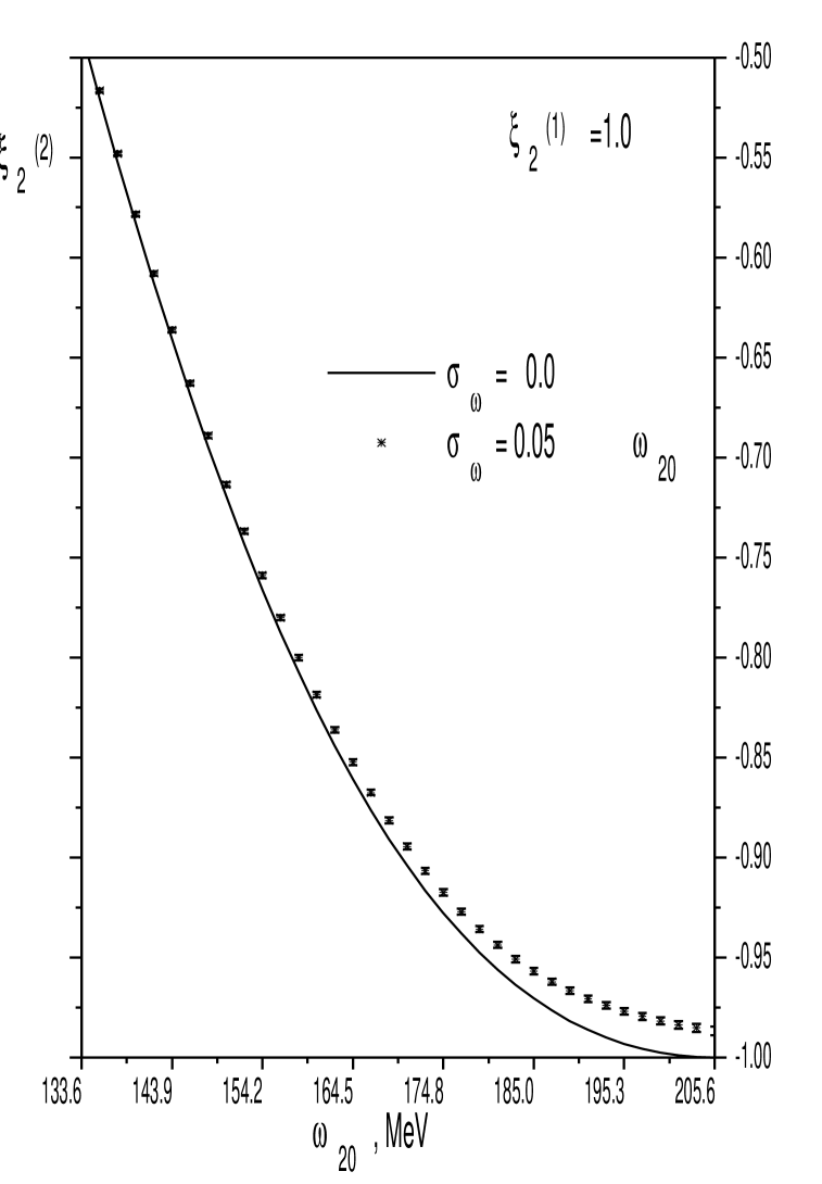
Figure 2: Averaged circular polarization of outgoing photon,
$\left\langle\xi_{3}^{(2)}\right\rangle$ versus $\omega_{20}$. $\xi_{2}^{(1)}=0,\xi_{1}^{(1)}=0,\xi_{3}^{(1)}=1.0$.
Number of simulated events – $10^{6}$ for each value $\omega_{20}.$

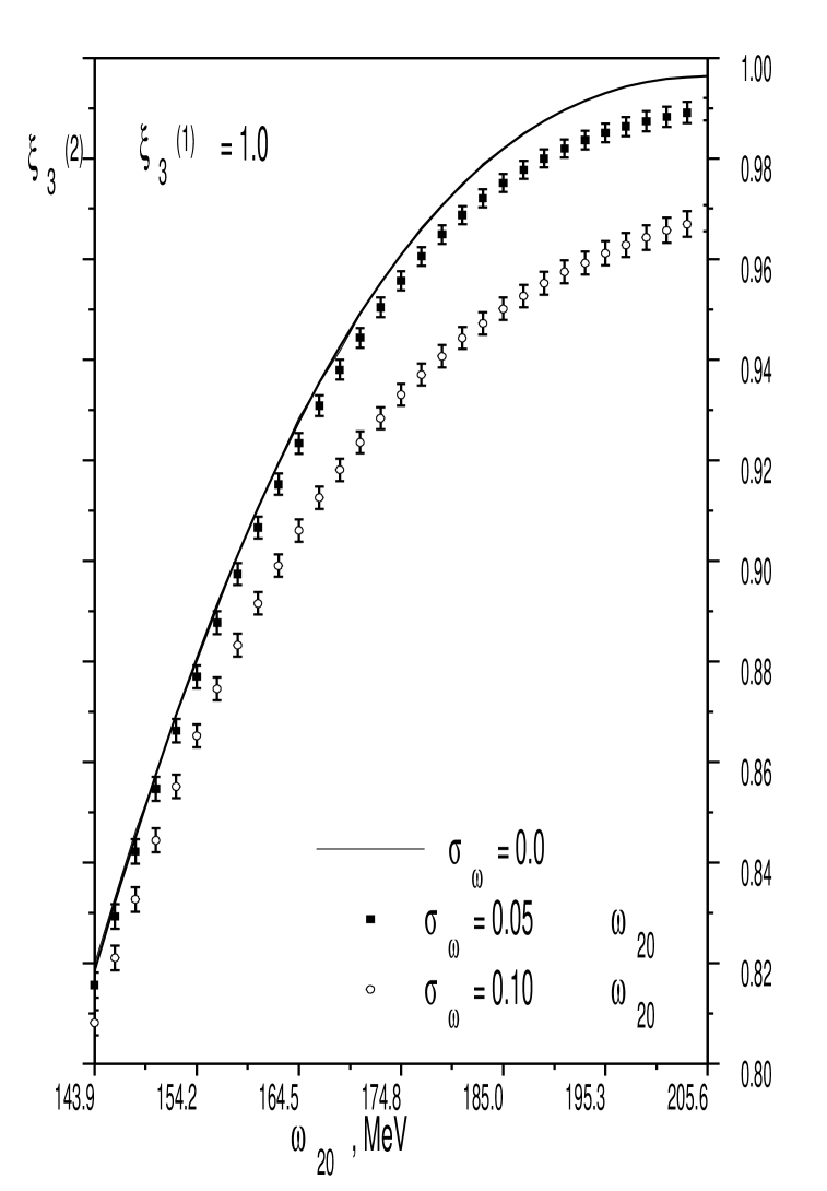
Figure 3: Averaged linear polarization of outgoing photon,
$\left\langle\xi_{3}^{(2)}\right\rangle$ versus $\omega_{20}$. $\xi_{2}^{(1)}=0,\xi_{1}^{(1)}=0,\xi_{3}^{(1)}=1.0$.
Number of simulated events – $10^{6}$ for each value $\omega_{20}.$

References

• [1] Sesler A.M. Physics today, v.5, p.48 (1998)
• [2] M.Anghinolfi et.al., Report GRAAL , ISN 9331 (Grenoble), IPNO-DRE 9309 (Orsay)
• [3] Harutyunian F.R., Tumanian V.A., JETP, v.44, p.2100 (1963)
• [4] Harutyunian F.R., Tumanian V.A.,Phys. Rev. Lett., v.4,p.176 (1963)
• [5] Millborn R.H., Phys. Rev. Lett., v.10, p.75 (1963)
• [6] Fano U.J. Opt. Soc. Am., v.39, p.859 (1949)
• [7] A.I. Akhiezer, V.B. Berestetskii, Quantum Electrodynamics. (Fizmatgiz, M., 1959)
• [8] Babusci B., Giordano G., Matone G. ”Polarization Effects in Electron Compton Scattering” INFN - Laboratory Nationali di Frascati, Italy. Preprint LNF - 95/004(IR), 1995.
• [9] Grinchishin Ya.T.,Scattering of Laser Photons on Relativistic Electrons with Arbitrary Polarization/. Journ. Nucl. Phys.,v.36,p.1450-1456 (1982).
• [10] V.B. Berestetskii, E.M. Lifschits and L.P, Pitaevskii, Quantum Electrodynamics. (Pergamon Press, N.Y.,1982)
• [11] R.G.Newton., Scattering Theory of Waves and Particles (McGraw-Hill,1965)
Refer to caption