A Multilevel Blocking Approach to the Sign Problem in Real-Time Quantum Monte Carlo Simulations

Abstract

We propose a novel approach toward the general solution of the sign problem in real-time path-integral simulations. Using a recursive multilevel blocking strategy, this method circumvents the sign problem by synthesizing the phase cancellations arising from interfering quantum paths on multiple timescales. A number of numerical examples with one or a few explicit degrees of freedom illustrate the usefulness of the method.

Path integrals [1] provide an elegant alternative to the operator formulation of quantum mechanics. Because they are easily adapted to many-body systems, quantum Monte Carlo (QMC) simulations based on path integrals can potentially yield exact results for the dynamics of condensed phase quantum systems. A number of early attempts to use QMC simulations for real-time dynamics [2] demonstrated their potential, but these studies also uncovered the ubiquitous “dynamical sign problem” — interference among quantum paths leads to large statistical noise that increases linearly with the number of possible paths, which in turn grows exponentially with the timescale of the problem. Consequently, real-time QMC simulations have been limited to problems of very short timescales. Several attempts to extend the timescale of real-time QMC simulations have appeared [3, 4, 5], all of which rely on a common idea — by using various filtering schemes, the phase cancellations can be numerically stabilized by damping out the non-stationary regions in configuration space. Such filtering methods were able to extend the timescale somewhat, but they were generally unable to reach timescales of interest in typical chemical systems.

Here we propose a novel approach based on a blocking strategy which may provide a general solution to the dynamical sign problem for very long times. The blocking strategy asserts that by sampling groups of paths called blocks, the sign problem is always reduced compared to sampling single paths [6]. Though this blocking strategy seems simple, its practical implementation is cumbersome, especially when going out to long times. Because the number of paths grows exponentially with the timescale, the number of blocks also grows immensely. To cure this problem, we first define elementary blocks and then group them together into larger blocks. Blocks of different sizes are introduced on several timescales called levels. After taking care of the sign cancellations within all blocks on a finer level, the entire sign problem can then be transferred to the next coarser level. By recursively proceeding from the bottom level (shortest timescale) up to the top (longest timescale), the troublesome numerical instabilities associated with the sign problem can be systematically avoided. In a slightly different form, this multilevel blocking (MLB) algorithm has recently been applied to treat the “fermion sign problem” in many-fermion imaginary-time simulations [7]. As most technical details of the MLB scheme can be found in [7], we only give a brief description of the algorithm below, stressing the main ideas and its differences from the fermion formulation.

For concreteness, we describe the MLB method for the calculation of an equilibrium time-correlation function,

$$\langle A(0)B(t)\rangle=\frac{{\rm Tr}\left\{e^{-(\beta\hbar+it)H/\hbar}Ae^{+itH/\hbar}B\right\}}{{\rm Tr}\left\{e^{-(\beta\hbar+it)H/\hbar}e^{+itH/\hbar}\right\}}\;.$$ (1)

With minor modifications, the MLB method also applies to other dynamical properties like the thermally symmetrized correlation function [8], $C_{s}(t)=Z^{-1}{\rm Tr}\{e^{-(\beta\hbar/2+it)H/\hbar}Ae^{-(\beta/\hbar/2-it)H/\hbar}B\}$, with $Z$ being the partition function. In terms of path integrals, the traces in (1) involve two quantum paths, one propagated backward in time for the duration $-t$ and the other propagated in complex time for the duration $t-i\beta\hbar$. Discretizing each of the two paths into $P$ slices, the entire cyclic path has a total of $2P$ slices. A slice on the first half of them has length $-t/P$, and on the second half $(t-i\beta\hbar)/P$. We require $P=2^{L}$ which defines the total number of levels $L$. Denoting the quantum numbers (e.g., spin or position variables) at slice $j$ by $\mathchoice{{\hbox{\boldmath$\displaystyle r$}}}{{\hbox{\boldmath$\textstyle r$}}}{{\hbox{\boldmath$\scriptstyle r$}}}{{\hbox{\boldmath$\scriptscriptstyle r$}}}_{j}$, $\{\mathchoice{{\hbox{\boldmath$\displaystyle r$}}}{{\hbox{\boldmath$\textstyle r$}}}{{\hbox{\boldmath$\scriptstyle r$}}}{{\hbox{\boldmath$\scriptscriptstyle r$}}}_{1},\cdots\mathchoice{{\hbox{\boldmath$\displaystyle r$}}}{{\hbox{\boldmath$\textstyle r$}}}{{\hbox{\boldmath$\scriptstyle r$}}}{{\hbox{\boldmath$\scriptscriptstyle r$}}}_{2P}\}$ is a discrete representation of a path, and the correlation function (1) reads

$$\frac{\int d\mathchoice{{\hbox{\boldmath$\displaystyle r$}}}{{\hbox{\boldmath$\textstyle r$}}}{{\hbox{\boldmath$\scriptstyle r$}}}{{\hbox{\boldmath$\scriptscriptstyle r$}}}_{1}\cdots d\mathchoice{{\hbox{\boldmath$\displaystyle r$}}}{{\hbox{\boldmath$\textstyle r$}}}{{\hbox{\boldmath$\scriptstyle r$}}}{{\hbox{\boldmath$\scriptscriptstyle r$}}}_{2P}B(\mathchoice{{\hbox{\boldmath$\displaystyle r$}}}{{\hbox{\boldmath$\textstyle r$}}}{{\hbox{\boldmath$\scriptstyle r$}}}{{\hbox{\boldmath$\scriptscriptstyle r$}}}_{2P})A(\mathchoice{{\hbox{\boldmath$\displaystyle r$}}}{{\hbox{\boldmath$\textstyle r$}}}{{\hbox{\boldmath$\scriptstyle r$}}}{{\hbox{\boldmath$\scriptscriptstyle r$}}}_{P})\prod_{j=1}^{2P}(\mathchoice{{\hbox{\boldmath$\displaystyle r$}}}{{\hbox{\boldmath$\textstyle r$}}}{{\hbox{\boldmath$\scriptstyle r$}}}{{\hbox{\boldmath$\scriptscriptstyle r$}}}_{j},\mathchoice{{\hbox{\boldmath$\displaystyle r$}}}{{\hbox{\boldmath$\textstyle r$}}}{{\hbox{\boldmath$\scriptstyle r$}}}{{\hbox{\boldmath$\scriptscriptstyle r$}}}_{j+1})_{0}}{\int d\mathchoice{{\hbox{\boldmath$\displaystyle r$}}}{{\hbox{\boldmath$\textstyle r$}}}{{\hbox{\boldmath$\scriptstyle r$}}}{{\hbox{\boldmath$\scriptscriptstyle r$}}}_{1}\cdots d\mathchoice{{\hbox{\boldmath$\displaystyle r$}}}{{\hbox{\boldmath$\textstyle r$}}}{{\hbox{\boldmath$\scriptstyle r$}}}{{\hbox{\boldmath$\scriptscriptstyle r$}}}_{2P}\prod_{j=1}^{2P}(\mathchoice{{\hbox{\boldmath$\displaystyle r$}}}{{\hbox{\boldmath$\textstyle r$}}}{{\hbox{\boldmath$\scriptstyle r$}}}{{\hbox{\boldmath$\scriptscriptstyle r$}}}_{j},\mathchoice{{\hbox{\boldmath$\displaystyle r$}}}{{\hbox{\boldmath$\textstyle r$}}}{{\hbox{\boldmath$\scriptstyle r$}}}{{\hbox{\boldmath$\scriptscriptstyle r$}}}_{j+1})_{0}}\;,$$ (2)

where the level-0 bond $(\mathchoice{{\hbox{\boldmath$\displaystyle r$}}}{{\hbox{\boldmath$\textstyle r$}}}{{\hbox{\boldmath$\scriptstyle r$}}}{{\hbox{\boldmath$\scriptscriptstyle r$}}}_{j},\mathchoice{{\hbox{\boldmath$\displaystyle r$}}}{{\hbox{\boldmath$\textstyle r$}}}{{\hbox{\boldmath$\scriptstyle r$}}}{{\hbox{\boldmath$\scriptscriptstyle r$}}}_{j+1})_{0}$ is simply the short-time propagator between slices $j$ and $j+1$, and $\mathchoice{{\hbox{\boldmath$\displaystyle r$}}}{{\hbox{\boldmath$\textstyle r$}}}{{\hbox{\boldmath$\scriptstyle r$}}}{{\hbox{\boldmath$\scriptscriptstyle r$}}}_{2P+1}=\mathchoice{{\hbox{\boldmath$\displaystyle r$}}}{{\hbox{\boldmath$\textstyle r$}}}{{\hbox{\boldmath$\scriptstyle r$}}}{{\hbox{\boldmath$\scriptscriptstyle r$}}}_{1}$. A direct application of the QMC method would sample these paths using the modulus of the integrand in the denominator as the weight.

We first assign all slices along the discretized path to different levels $\ell=0,\ldots,L$ (see Figure 1). Each slice $j=1,\ldots,2P$ belongs to a unique level $\ell$, such that $j=(2k+1)2^{\ell}$ and $k$ is a nonnegative integer. For instance, slices $j=1,3,5,\ldots$ belong to level $\ell=0$, slices $j=2,6,10,\ldots$ to $\ell=1$, etc. The MLB algorithm starts by sampling only configurations which are allowed to vary on slices associated with the finest level $\ell=0$, using the weight ${\cal P}_{0}=|(\mathchoice{{\hbox{\boldmath$\displaystyle r$}}}{{\hbox{\boldmath$\textstyle r$}}}{{\hbox{\boldmath$\scriptstyle r$}}}{{\hbox{\boldmath$\scriptscriptstyle r$}}}_{1},\mathchoice{{\hbox{\boldmath$\displaystyle r$}}}{{\hbox{\boldmath$\textstyle r$}}}{{\hbox{\boldmath$\scriptstyle r$}}}{{\hbox{\boldmath$\scriptscriptstyle r$}}}_{2})_{0}\cdots(\mathchoice{{\hbox{\boldmath$\displaystyle r$}}}{{\hbox{\boldmath$\textstyle r$}}}{{\hbox{\boldmath$\scriptstyle r$}}}{{\hbox{\boldmath$\scriptscriptstyle r$}}}_{2P},\mathchoice{{\hbox{\boldmath$\displaystyle r$}}}{{\hbox{\boldmath$\textstyle r$}}}{{\hbox{\boldmath$\scriptstyle r$}}}{{\hbox{\boldmath$\scriptscriptstyle r$}}}_{1})_{0}|$. The short-time level-$0$ bonds are then employed to synthesize longer-time level-$1$ bonds that connect the even-$j$ slices. Subsequently the level-1 bonds are used to synthesize level-$2$ bonds, and so on. In this way the MLB algorithm moves recursively from the finest level ($\ell=0$) up to increasingly coarser levels until $\ell=L$, where the measurement is done using $\mathchoice{{\hbox{\boldmath$\displaystyle r$}}}{{\hbox{\boldmath$\textstyle r$}}}{{\hbox{\boldmath$\scriptstyle r$}}}{{\hbox{\boldmath$\scriptscriptstyle r$}}}_{2P}$ and $\mathchoice{{\hbox{\boldmath$\displaystyle r$}}}{{\hbox{\boldmath$\textstyle r$}}}{{\hbox{\boldmath$\scriptstyle r$}}}{{\hbox{\boldmath$\scriptscriptstyle r$}}}_{P}$.

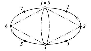
FIG. 1.: Example of how slices (circles) are assigned to various levels for $L=2$. The first path goes from $j=8$ to $4$ and the second from $j=4$ to $8$. The finest level $\ell=0$ contains $j=1,3,5,7$, level $\ell=1$ contains $j=2,6$, and the top level $\ell=2$ contains $j=4,8$. Coarse bonds are indicated by dotted (level-1) and dashed (level-2) lines.

Generating a MC trajectory containing $K$ samples for each slice on level $\ell=0$ and storing these samples, we compute the level-1 bonds according to

$$(\mathchoice{{\hbox{\boldmath$\displaystyle r$}}}{{\hbox{\boldmath$\textstyle r$}}}{{\hbox{\boldmath$\scriptstyle r$}}}{{\hbox{\boldmath$\scriptscriptstyle r$}}}_{j},\mathchoice{{\hbox{\boldmath$\displaystyle r$}}}{{\hbox{\boldmath$\textstyle r$}}}{{\hbox{\boldmath$\scriptstyle r$}}}{{\hbox{\boldmath$\scriptscriptstyle r$}}}_{j+2})_{1} = \langle{\Phi}[(\mathchoice{{\hbox{\boldmath$\displaystyle r$}}}{{\hbox{\boldmath$\textstyle r$}}}{{\hbox{\boldmath$\scriptstyle r$}}}{{\hbox{\boldmath$\scriptscriptstyle r$}}}_{j},\mathchoice{{\hbox{\boldmath$\displaystyle r$}}}{{\hbox{\boldmath$\textstyle r$}}}{{\hbox{\boldmath$\scriptstyle r$}}}{{\hbox{\boldmath$\scriptscriptstyle r$}}}_{j+1})_{0}(\mathchoice{{\hbox{\boldmath$\displaystyle r$}}}{{\hbox{\boldmath$\textstyle r$}}}{{\hbox{\boldmath$\scriptstyle r$}}}{{\hbox{\boldmath$\scriptscriptstyle r$}}}_{j+1},\mathchoice{{\hbox{\boldmath$\displaystyle r$}}}{{\hbox{\boldmath$\textstyle r$}}}{{\hbox{\boldmath$\scriptstyle r$}}}{{\hbox{\boldmath$\scriptscriptstyle r$}}}_{j+2})_{0}]\rangle_{{\cal P}_{0}}$$ (3)

$$= K^{-1}\sum_{\mathchoice{{\hbox{\boldmath$\displaystyle r$}}}{{\hbox{\boldmath$\textstyle r$}}}{{\hbox{\boldmath$\scriptstyle r$}}}{{\hbox{\boldmath$\scriptscriptstyle r$}}}_{j+1}}{\Phi}[(\mathchoice{{\hbox{\boldmath$\displaystyle r$}}}{{\hbox{\boldmath$\textstyle r$}}}{{\hbox{\boldmath$\scriptstyle r$}}}{{\hbox{\boldmath$\scriptscriptstyle r$}}}_{j},\mathchoice{{\hbox{\boldmath$\displaystyle r$}}}{{\hbox{\boldmath$\textstyle r$}}}{{\hbox{\boldmath$\scriptstyle r$}}}{{\hbox{\boldmath$\scriptscriptstyle r$}}}_{j+1})_{0}(\mathchoice{{\hbox{\boldmath$\displaystyle r$}}}{{\hbox{\boldmath$\textstyle r$}}}{{\hbox{\boldmath$\scriptstyle r$}}}{{\hbox{\boldmath$\scriptscriptstyle r$}}}_{j+1},\mathchoice{{\hbox{\boldmath$\displaystyle r$}}}{{\hbox{\boldmath$\textstyle r$}}}{{\hbox{\boldmath$\scriptstyle r$}}}{{\hbox{\boldmath$\scriptscriptstyle r$}}}_{j+2})_{0}]\;,$$ (4)

where the summation $\sum_{\mathchoice{{\hbox{\boldmath$\displaystyle r$}}}{{\hbox{\boldmath$\textstyle r$}}}{{\hbox{\boldmath$\scriptstyle r$}}}{{\hbox{\boldmath$\scriptscriptstyle r$}}}_{j+1}}$ extends over the $K$ samples, and $\Phi[z]=e^{i{\rm arg}(z)}$ denotes the phase. For a complete solution of the sign problem, the sample number $K$ has to be sufficiently large [7]. The bonds (3) contain crucial information about the sign cancellations on the previous level $\ell=0$. Their benefit becomes clear when rewriting the integrand of the denominator in (2) as

$\displaystyle{\cal P}_{0}\,\times\,(\mathchoice{{\hbox{\boldmath$\displaystyle r$}}}{{\hbox{\boldmath$\textstyle r$}}}{{\hbox{\boldmath$\scriptstyle r$}}}{{\hbox{\boldmath$\scriptscriptstyle r$}}}_{2},\mathchoice{{\hbox{\boldmath$\displaystyle r$}}}{{\hbox{\boldmath$\textstyle r$}}}{{\hbox{\boldmath$\scriptstyle r$}}}{{\hbox{\boldmath$\scriptscriptstyle r$}}}_{4})_{1}\cdots(\mathchoice{{\hbox{\boldmath$\displaystyle r$}}}{{\hbox{\boldmath$\textstyle r$}}}{{\hbox{\boldmath$\scriptstyle r$}}}{{\hbox{\boldmath$\scriptscriptstyle r$}}}_{2P-2},\mathchoice{{\hbox{\boldmath$\displaystyle r$}}}{{\hbox{\boldmath$\textstyle r$}}}{{\hbox{\boldmath$\scriptstyle r$}}}{{\hbox{\boldmath$\scriptscriptstyle r$}}}_{2P})_{1}(\mathchoice{{\hbox{\boldmath$\displaystyle r$}}}{{\hbox{\boldmath$\textstyle r$}}}{{\hbox{\boldmath$\scriptstyle r$}}}{{\hbox{\boldmath$\scriptscriptstyle r$}}}_{2P},\mathchoice{{\hbox{\boldmath$\displaystyle r$}}}{{\hbox{\boldmath$\textstyle r$}}}{{\hbox{\boldmath$\scriptstyle r$}}}{{\hbox{\boldmath$\scriptscriptstyle r$}}}_{2})_{1}\;.$

Comparing this to (2), we notice that the entire sign problem has been transferred to the next coarser level.

In the next step, the sampling is carried out on level $\ell=1$ in order to compute the next-level bonds, using the weight ${\cal P}_{0}{\cal P}_{1}$ with ${\cal P}_{1}=|(\mathchoice{{\hbox{\boldmath$\displaystyle r$}}}{{\hbox{\boldmath$\textstyle r$}}}{{\hbox{\boldmath$\scriptstyle r$}}}{{\hbox{\boldmath$\scriptscriptstyle r$}}}_{2},\mathchoice{{\hbox{\boldmath$\displaystyle r$}}}{{\hbox{\boldmath$\textstyle r$}}}{{\hbox{\boldmath$\scriptstyle r$}}}{{\hbox{\boldmath$\scriptscriptstyle r$}}}_{4})_{1}\cdots(\mathchoice{{\hbox{\boldmath$\displaystyle r$}}}{{\hbox{\boldmath$\textstyle r$}}}{{\hbox{\boldmath$\scriptstyle r$}}}{{\hbox{\boldmath$\scriptscriptstyle r$}}}_{2P},\mathchoice{{\hbox{\boldmath$\displaystyle r$}}}{{\hbox{\boldmath$\textstyle r$}}}{{\hbox{\boldmath$\scriptstyle r$}}}{{\hbox{\boldmath$\scriptscriptstyle r$}}}_{2})_{1}|$. Generating a sequence of $K$ samples for each slice on level $\ell=1$, and storing these samples, we then calculate the level-2 bonds in analogy with (3),

$\displaystyle(\mathchoice{{\hbox{\boldmath$\displaystyle r$}}}{{\hbox{\boldmath$\textstyle r$}}}{{\hbox{\boldmath$\scriptstyle r$}}}{{\hbox{\boldmath$\scriptscriptstyle r$}}}_{j},\mathchoice{{\hbox{\boldmath$\displaystyle r$}}}{{\hbox{\boldmath$\textstyle r$}}}{{\hbox{\boldmath$\scriptstyle r$}}}{{\hbox{\boldmath$\scriptscriptstyle r$}}}_{j+4})_{2}=\langle{\Phi}\left[(\mathchoice{{\hbox{\boldmath$\displaystyle r$}}}{{\hbox{\boldmath$\textstyle r$}}}{{\hbox{\boldmath$\scriptstyle r$}}}{{\hbox{\boldmath$\scriptscriptstyle r$}}}_{j},\mathchoice{{\hbox{\boldmath$\displaystyle r$}}}{{\hbox{\boldmath$\textstyle r$}}}{{\hbox{\boldmath$\scriptstyle r$}}}{{\hbox{\boldmath$\scriptscriptstyle r$}}}_{j+2})_{1}(\mathchoice{{\hbox{\boldmath$\displaystyle r$}}}{{\hbox{\boldmath$\textstyle r$}}}{{\hbox{\boldmath$\scriptstyle r$}}}{{\hbox{\boldmath$\scriptscriptstyle r$}}}_{j+2},\mathchoice{{\hbox{\boldmath$\displaystyle r$}}}{{\hbox{\boldmath$\textstyle r$}}}{{\hbox{\boldmath$\scriptstyle r$}}}{{\hbox{\boldmath$\scriptscriptstyle r$}}}_{j+4})_{1}\right]\rangle_{{\cal P}_{0}{\cal P}_{1}}\;,$

and iterate the process up to the top level by employing analogously defined level-$\ell$ bonds. The correlation function (1) can then be computed from

$$\frac{\langle B(\mathchoice{{\hbox{\boldmath$\displaystyle r$}}}{{\hbox{\boldmath$\textstyle r$}}}{{\hbox{\boldmath$\scriptstyle r$}}}{{\hbox{\boldmath$\scriptscriptstyle r$}}}_{2P})A(\mathchoice{{\hbox{\boldmath$\displaystyle r$}}}{{\hbox{\boldmath$\textstyle r$}}}{{\hbox{\boldmath$\scriptstyle r$}}}{{\hbox{\boldmath$\scriptscriptstyle r$}}}_{P}){\Phi}[(\mathchoice{{\hbox{\boldmath$\displaystyle r$}}}{{\hbox{\boldmath$\textstyle r$}}}{{\hbox{\boldmath$\scriptstyle r$}}}{{\hbox{\boldmath$\scriptscriptstyle r$}}}_{P},\mathchoice{{\hbox{\boldmath$\displaystyle r$}}}{{\hbox{\boldmath$\textstyle r$}}}{{\hbox{\boldmath$\scriptstyle r$}}}{{\hbox{\boldmath$\scriptscriptstyle r$}}}_{2P})_{L}(\mathchoice{{\hbox{\boldmath$\displaystyle r$}}}{{\hbox{\boldmath$\textstyle r$}}}{{\hbox{\boldmath$\scriptstyle r$}}}{{\hbox{\boldmath$\scriptscriptstyle r$}}}_{2P},\mathchoice{{\hbox{\boldmath$\displaystyle r$}}}{{\hbox{\boldmath$\textstyle r$}}}{{\hbox{\boldmath$\scriptstyle r$}}}{{\hbox{\boldmath$\scriptscriptstyle r$}}}_{P})_{L}]\rangle_{\cal P}}{\langle{\Phi}[(\mathchoice{{\hbox{\boldmath$\displaystyle r$}}}{{\hbox{\boldmath$\textstyle r$}}}{{\hbox{\boldmath$\scriptstyle r$}}}{{\hbox{\boldmath$\scriptscriptstyle r$}}}_{P},\mathchoice{{\hbox{\boldmath$\displaystyle r$}}}{{\hbox{\boldmath$\textstyle r$}}}{{\hbox{\boldmath$\scriptstyle r$}}}{{\hbox{\boldmath$\scriptscriptstyle r$}}}_{2P})_{L}(\mathchoice{{\hbox{\boldmath$\displaystyle r$}}}{{\hbox{\boldmath$\textstyle r$}}}{{\hbox{\boldmath$\scriptstyle r$}}}{{\hbox{\boldmath$\scriptscriptstyle r$}}}_{2P},\mathchoice{{\hbox{\boldmath$\displaystyle r$}}}{{\hbox{\boldmath$\textstyle r$}}}{{\hbox{\boldmath$\scriptstyle r$}}}{{\hbox{\boldmath$\scriptscriptstyle r$}}}_{P})_{L}]\rangle_{\cal P}}\;,$$ (5)

with the positive definite MC weight ${\cal P}={\cal P}_{0}{\cal P}_{1}\cdots{\cal P}_{L}$. The denominator in (5) gives the average phase and indicates to what extent the sign problem has been solved. Under the direct QMC method, the average phase decays exponentially with $t$ and is typically close to zero. With the MLB algorithm, however, the average phase remains close to unity even for long times, with a CPU time requirement $\sim t$. The price to pay for the stability of the algorithm is the increased memory requirement $\sim K^{2}$ associated with having to store the sampled configurations.

Now we illustrate the practical usefulness of the MLB method by several numerical examples. In each of these examples, we compute a time-correlation function. The average phase is larger than 0.6 for all data sets shown below. The decay in the average phase with $t$ is a result of the finiteness of $K$ [7]. Choosing a larger $K$ allows for a larger average phase out to longer time at the cost of increased computer memory and CPU time. Each data point in even the most intensive calculation took no more than a few hours on an IBM RS 6000/590.

A. Harmonic oscillator. For $H=p^{2}/2m+m\omega^{2}x^{2}/2$, the real and imaginary parts of $\langle x(0)x(t)\rangle$ oscillate in time due to vibrational coherence. In dimensionless units $m=\omega=1$, the oscillation period is $2\pi$. Figure 2(a) shows MLB results for $C(t)={\rm Re}\,\langle x(0)x(t)\rangle$. With $P=32$ for the maximum time $t=26$, $K=200$ samples were used for sampling the coarser bonds. Within error bars, the data coincide with the exact result and the algorithm produces stable results free of the sign problem. Without MLB, the signal-to-noise ratio was practically zero for $t>2$.

B. Two-level system. For a symmetric two-state system, $H=-\frac{1}{2}\Delta\sigma_{x}$, the dynamics is controlled by tunneling. The spin correlation function $\langle\sigma_{z}(0)\sigma_{z}(t)\rangle$ exhibits oscillations indicative of quantum coherence. Figure 2(b) shows MLB results for $C(t)={\rm Re}\,\langle\sigma_{z}(0)\sigma_{z}(t)\rangle$, Putting $\Delta=1$, the tunneling oscillations have a period of $2\pi$. With $P=64$ for the maximum time $t=64$, only $K=100$ samples were used for sampling the coarser bonds. The data agree well with the exact result. Again the simulation is stable and free of the sign problem. Without MBL, the simulation failed for $t>4$.

FIG. 2.: MLB results (closed circles) for various systems. Error bars indicate one standard deviation. (a) $C(t)$ for a harmonic oscillator at $\beta\hbar=1$. The exact result is indicated by the solid curve. (b) Same as (a) for a two-level system at $\beta\hbar=10$. (c) Same as (a) for a double-well system at $\beta\hbar=1$. This temperature corresponds to the classical barrier energy. (d) $C^{\prime}_{s}(t)$ for a double-well system coupled to two oscillators at $\beta\hbar=1$. For comparison, open diamonds are for the uncoupled $(\alpha=0)$ system. Note that $C^{\prime}_{s}(t)$ is similar but not identical to $C(t)$ shown in (c). Solid and dashed lines are guides to the eye only.

C. Double-well potential. Next, we examine a double-well system with the quartic potential $V(x)=-x^{2}+\frac{1}{4}x^{4}$. At low temperatures, interwell transfer occurs through tunneling motions on top of intrawell vibrations. These two effects combine to produce nontrivial structures in the position correlation function. At high temperatures, interwell transfer can also occur by classical barrier crossings. Figure 2(c) shows MLB results for $C(t)={\rm Re}\,\langle x(0)x(t)\rangle$. The slow oscillation corresponds to interwell tunneling, with a period of approximately 16. The higher-frequency motions are characteristic of intrawell oscillations. In this simulation, $K=300$ samples were used. The data reproduce the exact result well, capturing all the fine features of the oscillations. Again the calculation is stable and free of the sign problem, whereas a direct simulation failed for $t>3$.

D. Multidimensional tunneling system. As a final example, we consider a problem with three degrees of freedom, in which a particle in a double-well potential is bilinearly coupled to two harmonic oscillators. The quartic potential in the last example is used for the double-well, and the harmonic potential in the first example is used for both oscillators. The coupling constant between each oscillator and the tunneling particle is $\alpha=1/2$ in dimensionless units. For this example, we computed the correlation function $C_{s}(t)$ for the position operator of the tunneling particle. Direct application of MC sampling to $C_{s}(t)$ has generally been found unstable for $t>\beta\hbar/2$ [8]. In contrast, employing only moderate values of $K=400$ to 900, the MLB calculations allowed us to go up to $t=10\beta\hbar$. (Notice that this $K$ is no larger than three, i.e. the number of dimensions, times the $K$ needed for one-dimensional systems.) Figure 2(d) shows MLB results for $C^{\prime}_{s}(t)={\rm Re}\,C_{s}(t)$. For the coupled system, the position correlations have lost the coherent oscillations and instead decay monotonically with time. Coupling to the medium clearly damps the coherence and tends to localize the tunneling particle.

The data presented here demonstrate that the MLB method holds substantial promise toward an exact and stable simulation method for real-time quantum dynamics computations of many-dimensional systems up to timescales of practical interest. Instead of the exponentially vanishing signal-to-noise ratio in a ordinary application of the Monte Carlo method to real-time path integral problems, the MLB method has a CPU requirement that grows only linearly with time. Moreover, the data we have so far seem to suggest that the memory requirement $K$ also grows only linearly with the dimensionality of the system.

This research has been supported by the National Science Foundation under grants CHE-9257094 and CHE-9528121, by the Sloan Foundation, the Dreyfus Foundation, and by the Volkswagen-Stiftung.

REFERENCES

• [1] R.P. Feynman and A.R. Hibbs, Quantum Mechanics and Path Integrals (McGraw-Hill, New York, 1965).
• [2] For a review, see D. Thirumalai and B.J. Berne, Ann. Rev. Phys. Chem. 37, 401 (1986).
• [3] V.S. Filinov, Nucl. Phys. B 271, 717 (1986).
• [4] N. Makri and W.H. Miller, Chem. Phys. Lett. 139, 10 (1987); J. Chem. Phys. 89, 2170 (1988).
• [5] J.D. Doll, M.J. Gillan, and D.L. Freeman, Chem. Phys. Lett. 143, 277 (1988); J.D. Doll, T.L. Beck, and D.L. Freeman, J. Chem. Phys. 89, 5753 (1988).
• [6] C.H. Mak and R. Egger, Adv. Chem. Phys. 93, 39 (1996).
• [7] C.H. Mak, R. Egger, and H. Weber-Gottschick, Phys. Rev. Lett. (in press); see also cond-mat/9810002.
• [8] D. Thirumalai and B.J. Berne, J. Chem. Phys. 79, 5029 (1984); ibid. 81, 2512 (1984).