Instantaneous Pair Theory for High–Frequency Vibrational Energy Relaxation in Fluids

Abstract

Notwithstanding the long and distinguished history of studies of vibrational energy relaxation, exactly how it is that high frequency vibrations manage to relax in a liquid remains somewhat of a mystery. Both experimental and theoretical approaches seem to say that there is a natural frequency range associated with intermolecular motion in liquids, typically spanning no more than a few hundred $cm^{-1}$. Landau–Teller–like theories explain rather easily how a solvent can absorb any vibrational energy within this “band”, but how is it that molecules can rid themselves of superfluous vibrational energies significantly in excess of these values? In this paper we develop a theory for such processes based on the idea that the crucial liquid motions are those that most rapidly modulate the force on the vibrating coordinate — and that by far the most important of these motions are those involving what we have called the mutual nearest neighbors of the vibrating solute. Specifically, we suggest that whenever there is a single solvent molecule sufficiently close to the solute that the solvent and solute are each other’s nearest neighbors, then the instantaneous scattering dynamics of the solute–solvent pair alone suffices to explain the high frequency relaxation. This highly reduced version of the dynamics has implications for some of the previous theoretical formulations of this problem. Previous instantaneous–normal–mode theories allowed us to understand the origin of a band of liquid frequencies, and even had some success in predicting relaxation within this band, but lacking a sensible picture of the effects of liquid anharmonicity on dynamics, were completely unable to treat higher frequency relaxation. When instantaneous–normal–mode dynamics is used to evaluate the instantaneous pair theory, though, we end up with a multiphonon picture of the relaxation which is in excellent agreement with the exact high-frequency dynamics — suggesting that the critical anharmonicity behind the relaxation is not in the complex, underlying liquid dynamics, but in the relatively easy–to–understand nonlinear solute–solvent coupling. There are implications, as well, for the Independent-Binary-Collision (IBC) theory of vibrational relaxation in liquids. The success of the instantaneous–pair approach certainly provides a measure of justification for the IBC model’s focus on few–body dynamics. However, the pair theory neither needs nor supports the basic IBC factoring of relaxation rates into many–body and few–body dynamical components — into collision rates and relaxation rates per collision. Rather, our results favor taking an instantaneous perspective: the relaxation rate is indeed exercise in few–body dynamics, but a different exercise for each instantaneous liquid configuration. The many–body features therefore appear only in the guise of a purely equilibrium problem, that of finding the liklihood of particularly effective solvent arrangements around the solute. All of these results are tested numerically on model diatomic solutes dissolved in atomic fluids (including the experimentally and theoretically interesting case of I₂ dissolved in Xe). The instantaneous pair theory leads to results in quantitative agreement with those obtained from far more laborious exact molecular dynamics simulations.

I Introduction

The most crucial step in a solution–phase chemical reaction is almost always a thermal activation; improbable as it may be, the solvent must find some avenue for concentrating enough of its kinetic energy within the vibrations of the reactants to allow the reaction to proceed. [1, 2] A similar challenge can be posed later on in the process; the ability of the resulting products to return any excess vibrational energy back to the solvent is often critical to the outcome of the reaction. [1, 3] Beyond these issues however, there is a conceptual importance to understanding such vibrational energy transfers that goes to the heart of how one thinks about the dynamical role of a solvent. If the entire solvent-solute system is regarded as a “super molecule” (as might be appropriate for solid-state vibrational relaxation), then the question is how a V–V relaxation occurs — that is, which vibrations of the system as a whole (which phonons) can serve as repositories for the solute’s vibrational energy. [4, 5, 6, 7] If, on the other hand, we consider the solute to be buffeted by occasional collisions with individual solvent molecules, a very natural perspective for the gas phase, what we need to understand is a V–T process. [8] So how is it that we should think about vibrational energy relaxation in liquids? [9, 10, 11, 12, 13, 14, 15, 16, 17, 18, 19, 20, 21, 22]

A formal answer to this question arises quite simply from a Fermi’s Golden Rule evaluation of the relaxation rate. [23] Within the apparently quite broad reach of low–order time–dependent perturbation theory, the rate at which vibrational energy relaxes from a given solute mode, $T_{1}^{-1}$, is proportional to the Fourier component of the autocorrelation function of the force on that mode at the mode’s own frequency, $\omega_{0}$. [24] For a diatomic molecule of reduced mass $\mu$, for example, the classical vibrational energy relaxation rate is predicted to obey the Landau–Teller formula, [14]

$${1\over T_{1}}\ =\ {1\over\mu}{\hat{\eta}}(\omega_{0})\ ,$$ (1)

where

$${\hat{\eta}}(\omega_{0})\ =\ \int_{0}^{\infty}dt\ \eta(t)\cos{\omega_{0}t}$$ (2)

(3)

$$\eta(t)\ =\ {1\over k_{B}T}\left<\delta F(t)\ \delta F(0)\right>\ .$$ (4)

Here $k_{B}$ is Boltzmann’s constant, $T$ is the temperature, and by $\delta F(t)=F(t)-F$, the fluctuating force on the mode, we mean the hypothetical classical time evolution of the solvent that would occur were the mode itself held motionless.

Leaving aside such issues as whether a purely classical treatment of the solvent can adequately represent the influence on what is frequently a rather quantum mechanical vibration, [25] it seems clear that this approach can usually be counted on to give a numerically accurate rendition of classical vibrational energy relaxation. [13] More than that, though, it provides a conceptually suggestive rendition because it fits so nicely into the broader context of relaxation in liquids. Within a Generalized Langevin representation of the problem, the function $\eta(t)$ can be interpreted as an approximation to the solvent-induced friction felt by a vibrating coordinate — and since the exact friction can sometimes be determined by simulation, it has been possible both to check and to understand the formalism’s accuracy. [12]

Still, the fact that numerical success does not necessarily translate into conceptual insight becomes clear once we try to get at the central V–V vs. V–T dichotomy. It has long been appreciated that any frequency–domain friction ${\hat{\eta}}(\omega)$ can be regarded as having its origin in the dynamics of a dense set of harmonic oscillators, oscillators whose frequencies span the frequency range of the friction and which are coupled linearly to the coordinate of interest. [26, 27] The fact that liquid frictions interpreted in this fashion typically have a spectrum spanning a few hundred $cm^{-1}$ could thus be taken as evidence that there is indeed something resembling a phonon band of this width in liquids. It is then but a short step to suggest that any vibrational relaxation of modes with frequencies lying within this band ought to be considered as occuring via a resonant V–V transfer.

This argument is actually rather weak as it stands. These harmonic oscillators could, in fact, be little more than mathematical constructs lacking any microscopic, molecular foundation. What gives the argument a bit more substance is that recent work has shown that it is possible to associate these oscillators with the instantaneous normal modes of the solutions, oscillators which really are specific, well–defined molecular motions. [28, 29, 30, 31, 32, 33, 34, 35] Indeed, perhaps it is fair to say that the basic success of such instantaneous–normal–mode (INM) approaches in predicting most of the essential behavior of the vibrational friction lends a certain amount of credibility to what would otherwise be fanciful attempts to take liquid phonon pictures literally in theories of vibrational relaxation. [36]

There is, however, a major problem and it is this problem that forms the topic of this paper. Once the vibration to be relaxed lies outside the putative band of the liquid, any theory with nothing but linear forces and harmonic oscillators will predict that energy relaxation is completely forbidden. [37] Yet, what we might call the high frequency modes of solutes (those with frequencies higher than the Debye frequency in the solid–state parlance) really do relax, albeit very slowly. [9, 17, 38] It is worth noting that the Landau–Teller formula itself has no difficulty with this phenomenon; it simply ascribes the relaxation to the presence of small but finite high–frequency Fourier components of the force autocorrelation function. [14] The conceptual difficulty is that we have independent evidence about the intrinsic bandwidth of intermolecular vibrations in a liquid, both from theoretical predictions, such as instantaneous–normal–mode analysis [39, 40, 41] and Fourier representations of simulated velocity autocorrelation functions [42] and from experimental results, such as those from far infrared, Rayleigh and Optical Kerr effect spectra. [43, 44] None of these estimates give any evidence that the band for simple liquids extends significantly beyond a few hundred $cm^{-1}$. A much more likely scenario than one that would require every simple liquid to have the kinds of 500–2000 $cm^{-1}$ intermolecular vibrations necessary for simple V–V processes is that high frequency vibrational energy relaxation is a strongly anharmonic event — and it is this anharmonicity we need to understand.

Having made this point, though, there is an interesting distinction we can make. The relaxation of impurity molecules in crystals can often be modeled as a multiphonon process, one in which the essential harmonicity of the vibrations (and hence the very idea of phonons) is respected, but in which the nonlinearity of the coupling forces allows for V-V transfer to overtones of the crystal’s intrinsic frequencies. [5, 6, 7, 45, 46] In systems as inherently anharmonic as liquids, however, we could easily imagine that the basic idea of independent harmonic excitations could be the first casualty. [47, 48, 49] Thus, without further work, it is far from clear which of these two kinds of anharmonicity — the nonlinearity of the forces being driven by the liquid’s dynamics or that of the actual dynamics itself — ought to be more critical to high–frequency relaxation in liquids. In particular, we are still left with the question of whether the V–V paradigm for resonant energy transfer is going to be any better than a V–T based perspective would be.

Complicating this issue is the fact that there is some evidence on the side of molecular translation being the primary sink for vibrational energy. That is, there is some support for a collisional model for vibrational relaxation. While it is admittedly far from intuitive how discrete, uncorrelated collisions could ever occur in a dense a medium as a liquid, the so–called Isolated–Binary Collision (IBC) model [50, 51] has been remarkably successful in rationalizing the thermodynamic state dependence of vibrational population relaxation rates based on just such a picture. [52, 53, 55] The notion behind this model is that these rates should factor into a purely few–body scattering piece specifying the rate of energy transfer per collision, and a liquid–state piece quantifying the rate at which the solvent collides with the solute. The fact that the concept (and thus the rate) of collisions is ill–defined in liquids is certainly vexing, [54, 55, 56] but it is hardly out of the question that some other, more sophisticated analysis of the collision concept might find that the V–T motif is still a dominant mechanism for relaxation.

The approach we shall take in this paper to getting at these issues is to begin with the standard perturbative (Landau–Teller) expression in terms of the force autocorrelation function, Eqs. (1)–(4), but then ask from precisely where we should expect the major high frequency components of the correlation function to arise. For any instantaneous configuration of the liquid, this analysis will immediately lead us to look at the short–time scattering dynamics of the solute and a single crucial solvent partner. Previous work on vibrational relaxation has shown that whenever there is a solvent molecule that is nearer to the solute than any other solvent molecule is to either member of the solute–solvent pair — that is, whenever there is a mutual–nearest–neighbor solute–solvent pair — then the high-frequency solvent effects are dominated by the pair, at least within the liquid’s band. [31] We will show how this observation can be exploited more generally, transcending the limitations to dynamics within the band. Not surprisingly, our theoretical prediction for the relaxation rate will then separate into a straightforward few–body dynamical calculation and a residual many–body problem, just as with IBC theory. However, unlike the IBC approach, the liquid–state portion of our theory will turn out to rest on a simple, well–defined, purely equilibrium question. Moreover, our development will make it clear how we can make connections between this V–T theory and the harmonic instantaneous dynamics of instantaneous–normal–modes, and thereby connect with the V–V energy transfer ideas which seem to work so well within the solvent band.

The remainder of the paper will be organized as follows: Section II will present our basic theory, an expression for the full force autocorrelation function of the system in terms of a correlation function for single degree of freedom, one whose equations of motion we proceed to derive. Section III then explores the connection to the instantaneous–normal–mode perspective, showing how we can view the new theory as a natural generalization of INM ideas. Section IV provides some numerical examples of how and how well the various approaches work, and we conclude in Sec. V with some general comments on what we are now in a position to say about the questions posed in this Introduction.

II Instantaneous Pair Theory for the Vibrational Friction

A Solute–Solvent Coupling versus Solute–Solvent Dynamics

While the central quantity of interest in vibrational relaxation is the force autocorrelation function of Eq. (4), it is convenient to look instead at a mathematically equivalent function, the “force–velocity” autocorrelation function, [57, 58]

$$G_{F}(t)\ =\ \left<{\dot{F}}(t)\ {\dot{F}}(0)\right>\ =\ -(k_{B}T)\ {\ddot{\eta}}(t)\ ,$$ (5)

which lets us write the frequency-domain vibrational friction we need in terms of the cosine transform of the new function [28, 29, 59]

$${\hat{\eta}}(\omega)\ =\ {1\over k_{B}T}\ \left({1\over\omega^{2}}\right)\int_{0}^{\infty}dt\ G_{F}(t)\ \cos{\omega t}\ \equiv\ {1\over k_{B}T}\ \left({{\hat{G}}_{F}(\omega)\over\omega^{2}}\right)\ .$$ (6)

The main reason we bother with this conversion is that this alternative version will suggest a natural division within our problem. As one might have expected, there will always be contributions from the relative solute–solvent velocities — the intrinsic dynamics of the problem — but there will be also be separate features dependent directly on the solute–solvent distances — and it is these that will be most pertinent to the solute–solvent coupling. [32] Indeed, one of the key aspects of our subsequent development will be the realization that these two kinds of information actually play substantially different roles in determining the high–frequency behavior.

We can begin to see how this division occurs by looking at the problem of evaluating a general correlation function of the form of Eq. (5) when $F$ is any specifically solute-centered quantity. That is, suppose we look at a correlation function of the form of Eq. (5) with the function $F$ given by a sum of solute-solvent pair “potentials”,

$$F\ =\ \sum_{j\ \in\ solvent}w(r_{0j})\ ,$$ (7)

with the tagged solute labeled as particle 0, the remaining solvent denoted by $j\ =\ 1,\ldots,\ N$ and the interparticle distances given by $r_{0j}\equiv|{\bf r_{0}}-{\bf r_{j}}|$, so that

$${\dot{F}}\ =\ \sum_{j\ \in\ solvent}w^{\prime}(r_{0j})\ {\dot{r}}_{0j}\ .$$ (8)

This general function $w(r)$, something we have referred to elsewhere as the “spectroscopic probe potential”, [32] could very well be the force on some portion of the solute (as it is in vibrational relaxation), but for the purposes of this argument it could also be the change in the solute-solvent potential energies when the solute is promoted from one electronic state to another (the situation in time-dependent fluorescence studies of solvation). [40]

If we substitute Eq. (8) into Eq. (5), we find that the velocity form of the correlation function consists of two kinds of terms,

$$G_{F}(t) = \left<\sum_{j}w^{\prime}[r_{0j}(t)]\ w^{\prime}[r_{0j}(0)]\ {\dot{r}}_{0j}(t)\ {\dot{r}}_{0j}(0)\right>$$ (9)

$$+ \left<\sum_{j,k\ (j\neq k)}w^{\prime}[r_{0j}(t)]\ w^{\prime}[r_{0k}(0)]\ {\dot{r}}_{0j}(t)\ {\dot{r}}_{0k}(0)\right>\ ,$$ (11)

a binary piece, the first term, which considers only the dynamics caused by the motion of a single solvent at a time, and a ternary piece, the second term, which involves the simultaneous motion of two different solvents.

These two parts will not contribute equally, for reasons we shall come to presently, but the essential ingredients of the correlation function are already visible. When we evaluate any of the terms at time $t=0$,

$$\left<w^{\prime}[r_{0j}(0)]\ w^{\prime}[r_{0k}(0)]\ {\dot{r}}_{0j}(0)\ {\dot{r}}_{0k}(0)\right> = \left<w^{\prime}[r_{0j}(0)]\ w^{\prime}[r_{0k}(0)]\right>\ \left<{\dot{r}}_{0j}(0)\ {\dot{r}}_{0k}(0)\right>$$ (12)

$$= \delta_{jk}\left<w^{\prime}[r_{0j}(0)]\ w^{\prime}[r_{0j}(0)]\right>\ \left<{\dot{r}}_{0j}(0)\ {\dot{r}}_{0j}(0)\right>\ ,$$ (14)

we notice that the contribution factors rigorously into a static part involving the coupling, $w^{\prime}(r)$, and a dynamical part involving the velocity, ${\dot{r}}$. This separation suggests, though, that this same conceptual distinction between coupling and dynamics ought to continue to operate at short times — and therefore at high frequencies — despite the fact that the expression no longer factors. But, once we make such a distinction, we can simplify our expressions dramatically. For one thing, at the highest frequencies we should expect coupling to be far more influential than dynamics in determining the correlation function. With typical intermolecular potentials and forces, the sharply varying repulsive parts allow for tremendous variation in the coupling (and therefore enormous values of $w^{\prime}(r))$ just from small changes in internuclear distances. The velocities, by contrast, never become all that large in magnitude, guided as they are by the equilibrium Boltzmann distribution.

We can make this same point a bit more quantitatively. If we assume that the $t=0$ factorization holds, at least roughly, then each term in $G_{F}(t)$ can be written

$$T_{jk}(t)\ = \ \left<w^{\prime}[r_{0j}(t)]\ w^{\prime}[r_{0k}(0)]\ {\dot{r}}_{0j}(t)\ {\dot{r}}_{0k}(0)\right>\$$ (15)

$$\approx \ \left<w^{\prime}[r_{0j}(t)]\ w^{\prime}[r_{0k}(0)]\right>\ \left<{\dot{r}}_{0j}(t)\ {\dot{r}}_{0k}(0)\right>\ ,$$ (17)

which becomes, on cosine transforming the resulting product,

$${\hat{T}}_{jk}\ \approx\ {\delta_{jk}\over\pi}\ \int_{0}^{\infty}d\omega^{\prime}\ {\hat{V}}(\omega^{\prime})\left[{\hat{C}}(\omega-\omega^{\prime})+{\hat{C}}(\omega+\omega^{\prime})\right]\ ,$$ (18)

where ${\hat{V}}(\omega)$ and ${\hat{C}}(\omega)$ are the cosine transforms of the single–solvent velocity and coupling correlation function, respectively. What then determines the high frequency behavior? The intrinsic frequencies of the liquid are largely those of ${\hat{V}}(\omega^{\prime})$, [42] which cuts off at frequencies $\omega^{\prime}$ well below the $\omega$ we are interested in. But if $\omega^{\prime}\ll\omega$, then ${\hat{C}}(\omega-\omega^{\prime})\ \approx{\hat{C}}(\omega)$, so

$$T_{jk}(\omega)\ \approx\ \delta_{jk}{2\over\pi}\left[\int_{0}^{\infty}d\omega^{\prime}\ {\hat{V}}(\omega^{\prime})\right]{\hat{C}}(\omega)\ .$$ (19)

Hence, we see again that the high–frequency dependence of our friction spectrum results almost entirely from the high-frequency behavior of the coupling.

This argument can be taken still further. The dynamic range of the coupling is so large that we might expect it to be dominated by the very largest contributions. No more than a few of the closest solvents should therefore play much of a role. Indeed, we might venture that only the single largest contribution, from the single most strongly coupled solvent is important, [31, 32]

$$G_{F}(t)\ =\ \left<w^{\prime}[r_{0j}(t)]\ w^{\prime}[r_{0j}(0)]\ {\dot{r}}_{0j}(t)\ {\dot{r}}_{0j}(0)\right>_{j=maximally\ coupled}\ .$$ (20)

What we suggest here is that this latter idea is virtually exact; that the high-frequency dynamics of a solute-centered correlation function stems almost entirely from the binary dynamics of a single solute-solvent pair — and all we need do is compute the nonlinear, anharmonic dynamics of this pair for each instantaneous liquid configuration.

There are actually a number of kinds of evidence supporting our analysis. An immediate consequence of our argument is that the binary terms in Eq. (11) ought to be significantly larger than the ternary terms at short times. Indeed, exact molecular dynamics simulations have established the overwhelming predominance of the binary contributions to the $G_{F}(t)$ vibrational relaxation correlation functions. [32] Interestingly, one finds the predicted strong preferences for the (presumably) less collective binary part even when the relaxation takes place in dipolar solvents, liquids whose intermolecular forces are sufficiently long–ranged that the friction $\eta(t)$ itself ends up with major contributions from ternary terms. [14, 32] The reasons for this difference between binary and ternary are clear from a short–time perspective. At equilibrium ($t=0$), the force–velocity version of the vibrational friction is rigorously binary, because, as we can see from Eq. (14), the velocities of different solvent molecules are rigorously independent. The actual equilibrium friction, by contrast, does not even start out as binary at $t=0$; the equilibrium structure of the liquid builds in correlations that have nothing to do with the subsequent dynamical evolution. But even away from $t=0$, the wide range of values possible for the couplings serves to explain the observation. The sheer unlikelihood of having two different solvents so similar in their distance from the solute that they end up making comparable contributions will also prevent much of a ternary presence in the answer.

We can see somewhat more direct evidence of the two-particle character of the essential dynamics by looking in the frequency domain with the aid of INM theory. INM theories cannot addresss any of the truly high-frequency dynamics, but if we confine ourselves to the highest frequencies inside the INM band, we invariably find that the vibrational friction spectrum ($\rho_{vib}(\omega)=(2/\pi){\hat{G}}_{F}(\omega)$) is given quantitatively by the portion arising from the motion of the solute and the single largest contributing solvent. [31, 32] Moreover, as with the molecular dynamics studies, these findings seems to be completely independent of how otherwise collective the solvent motion is. The question we are left with, therefore, is whether the nature of the relaxation really does change qualitatively as we cross the band edge. It does not seem all that far fetched for this same two–particle scenario that works so well just inside the band to apply at higher frequencies as well.

B The High-Frequency Parts of the Vibrational Relaxation Correlation Function

To make our subsequent development more concrete, suppose we specialize to the familiar case of a diatomic solute dissolved in an atomic liquid. Taking the atoms of the diatomic to be labeled as 1 and 2 (with masses $m_{1}$ and $m_{2}$), and indexing the atoms of the solvent by $j=3,\ \ldots,\ N$, we find that if the potential energy of interaction between the solute and the solvent can be written in terms of site-site pair potentials

$$V\ =\ \sum_{j>2}\left[u_{1}(r_{1j})+u_{2}(r_{2j})\right]\ ,$$ (21)

then the force acting on the diatomic’s bond is given by

$$F_{x}\ =\ -{\partial V\over\partial x}\ =\ \mu_{12}\sum_{j>2}\left[{1\over m_{1}}u^{\prime}_{1}(r_{1j}){\hat{\bf r}}_{1j}\ -\ {1\over m_{2}}u^{\prime}_{2}(r_{2j}){\hat{\bf r}}_{2j}\right]\cdot{\hat{\bf r}}_{12}\ .$$ (22)

Here $\mu_{12}=m_{1}m_{2}/(m_{1}+m_{2})$ is the solute reduced mass and ${\hat{\bf r}}={\bf r}/|{\bf r}|$. The requisite time derivative of the bond force is thus

$${\dot{F}}_{x}\ = \ \mu_{12}\sum_{j>2}\left[{1\over m_{1}}u^{\prime\prime}_{1}(r_{1j}){\dot{r}}_{1j}({\hat{\bf r}}_{1j}\cdot{\hat{\bf r}}_{12})\ -\ {1\over m_{2}}u^{\prime\prime}_{2}(r_{2j}){\dot{r}}_{2j}({\hat{\bf r}}_{2j}\cdot{\hat{\bf r}}_{12})\right]$$ (23)

$$+ \ \mu_{12}\sum_{j>2}\left[{1\over m_{1}}u^{\prime}_{1}(r_{1j}){d\over dt}({\hat{\bf r}}_{1j}\cdot{\hat{\bf r}}_{12})\ -\ {1\over m_{2}}u^{\prime}_{2}(r_{2j}){d\over dt}({\hat{\bf r}}_{2j}\cdot{\hat{\bf r}}_{12})\right]\ .$$ (25)

Let us now consider what the highest frequency parts of the force–velocity correlation function, Eq. (5), would look like for such a force. Generalizing our arguments in the previous section, we would expect that the dominant contribution would come (at most) from the two solvent atoms, call them $a$ and $b$, nearest the two solute sites 1 and 2 (respectively). [60] Furthermore, given the rapid variation of the site-site potentials $u_{1,2}(r)$ in the region of interest, we might also expect the terms involving the second derivative $u^{\prime\prime}(r)$ to be far more important than those involving the first derivative $u^{\prime}(r)$. Hence we should be able to express the correlation function as just

$$G_{F}(t)\ \approx \ \left({\mu_{12}\over m_{1}}\right)^{2}\left<u^{\prime\prime}(r_{1a}(t))\ u^{\prime\prime}(r_{1a}(0))\ \cos{\theta_{1a}(t)}\ \cos{\theta_{1a}(0)}\ {\dot{r}}_{1a}(t)\ {\dot{r}}_{1a}(0)\right>$$ (26)

$$+ \ \left({\mu_{12}\over m_{2}}\right)^{2}\left<u^{\prime\prime}(r_{2b}(t))\ u^{\prime\prime}(r_{2b}(0))\ \cos{\theta_{2b}(t)}\ \cos{\theta_{2b}(0)}\ {\dot{r}}_{2b}(t)\ {\dot{r}}_{2b}(0)\right>\ ,$$ (28)

with $\cos{\theta_{Aj}(t)}\equiv({\bf{\hat{r}}_{Aj}}\cdot{\bf{\hat{r}}_{12}})\ (A=1,2)$. We could, in fact, make use of Eq. (28) as it stands; since it requires that we know no more than the dynamics of 4 degrees of freedom, it already represents a major simplification over the full many–body problem. We can make one last simplification, however. The variation of the $\cos{\theta_{Aj}(t)}$ angular factors is also guaranteed to be far smaller than that of the $u^{\prime\prime}(r)$ factors at short times, if only because of the small dynamic range of the cosine function ($-1\leq\cos{\theta}\leq 1$). For the purposes of evaluating high–frequency behavior it therefore suffices to approximate the cosine by its $t=0$ value. Our final high–frequency expression for the vibrational relaxation correlation function thus reduces to a remarkably simple form

$$G_{F}(t)\ \approx \ \left({\mu_{12}\over m_{1}}\right)^{2}\left<u^{\prime\prime}(r_{1a}(t))\ u^{\prime\prime}(r_{1a}(0))\ \cos^{2}{\theta_{1a}(0)}\ {\dot{r}}_{1a}(t)\ {\dot{r}}_{1a}(0)\right>$$ (29)

$$+ \ \left({\mu_{12}\over m_{2}}\right)^{2}\left<u^{\prime\prime}(r_{2b}(t))\ u^{\prime\prime}(r_{2b}(0))\ \cos^{2}{\theta_{2b}(0)}\ {\dot{r}}_{2b}(t)\ {\dot{r}}_{2b}(0)\right>\ ,$$ (31)

relying only on the one–dimensional, purely radial dynamics of two solvent molecules moving with respect to the two solute sites.

C Mutual–Nearest–Neighbor Dynamics

Of course, since we are in a liquid, the exact dynamics of even this small a number of degrees of freedom is still intimately connected with the dynamics of the remainder. Were we unable to achieve any reduction of this dynamics comparable to the simplification we found for the correlation function, there would thus be little practical advantage to our formalism. Fortunately, the same kinds of analysis we have been pursuing also reveal a wonderful dynamical separability: the important solvents end up being dynamically decoupled from the rest of the solvent as well.

This basic notion of dynamical separability is illustrated by looking at the time evolution of a mutual–nearest–neighbor pair of atoms in an atomic liquid. [31, 49] The equations of motion for any two atoms $a$ and $b$, with masses $m_{a}$ and $m_{b}$, are

$$m_{a}{\bf{\ddot{r}}}_{a}\ = \ u^{\prime}(r_{ab}){\hat{\bf r}}_{ab}\ -\ \sum_{j\neq a,b}u^{\prime}(r_{aj}){\hat{\bf r}}_{ja}$$ (32)

$$m_{b}{\bf{\ddot{r}}}_{b}\ = \ -u^{\prime}(r_{ab}){\hat{\bf r}}_{ab}\ -\ \sum_{j\neq a,b}u^{\prime}(r_{bj}){\hat{\bf r}}_{jb}\ ,$$ (34)

provided all the atoms interact by pair potentials $u(r)$. But, if these two particular atoms form a mutual–nearest–neighbor pair, then $u^{\prime}(r_{ab})$ will be significantly larger than any of the other forces affecting the pair. Hence, to within a high level of accuracy, the relative acceleration will be given by

$${\bf{\ddot{r}}}_{ab}\ =\ {\bf{\ddot{r}}}_{b}\ -\ {\bf{\ddot{r}}}_{a}\ \approx\ -{1\over\mu}u^{\prime}(r_{ab}){\bf{\hat{r}}}_{ab}\ ,$$ (35)

meaning that the scalar displacement $r_{ab}$ will satisfy the differential equation

$${\ddot{r}}_{ab}\ =\ -{1\over\mu}u^{\prime}(r_{ab})\ +\ r_{ab}\Omega_{ab}^{2}\ ,$$ (36)

with $\mu=m_{a}m_{b}/(m_{a}+m_{b})$ the reduced mass of the pair. Here the angular velocity factor $\Omega_{ab}^{2}\equiv-{\bf{\hat{r}}}_{ab}\cdot{\bf{\ddot{\hat{r}}}}_{ab}$ and we have used the vector identity

$${\bf{\hat{r}}}_{ab}\cdot{\bf{\ddot{r}}}_{ab}\ =\ {\ddot{r}}_{ab}\ -\ r_{ab}\Omega_{ab}^{2}\ .$$ (37)

Equation (36) is intriguing, but it is not as simple as it may appear; the evolution of the centrifugal acceleration term $r_{ab}\Omega_{ab}^{2}$ is controlled by other forces besides $u^{\prime}(r_{ab})$ (and thus by the motion of other atoms besides $a$ and $b$). However it is fairly easy to see that this term too is almost always going to be negligible compared to the intra–pair force. We can estimate its size by using the equipartion theorem to get the mean–square angular velocity [61] $\Omega_{ab}^{2}=<\omega^{2}>=(k_{B}T/\mu r_{ab}^{2})$. If we take the pair potential to be of the Lennard–Jones form, $u(r)=4\epsilon[(\sigma/r)^{12}-(\sigma/r)^{6}]$, and we then make the (very) conservative estimate that a typical intra–pair distance $r_{ab}=\sigma$, we find that a typical value of the centrifugal force is $(k_{B}T/\epsilon)(\epsilon/\sigma)$, whereas a typical intermolecular force is $24(\epsilon/\sigma)$. Hence under any liquid–state conditions, indeed at anything other than the most extreme supercritical conditions, we can safely neglect such centrifugal contributions. [62] The dynamics of a mutual–nearest–neighbor pair of atoms is therefore well described by a simple, purely radial, equation of motion:

$${\ddot{r}}_{ab}\ =\ -{1\over\mu}u^{\prime}(r_{ab})\ ,$$ (38)

even in a dense liquid.

This same argument can easily be adapted to the vibrational relaxation example we considered in the last section. If only one atom (say number 1) of our diatomic solute forms a mutual nearest neighbor pair with a solvent atom (solvent $a$), then the equations of motion for the critical solvent atom and for ${\bf R}_{cm}$, the position of the diatomic’s center of mass, are given accurately by [63]

$$m_{a}{\bf{\ddot{r}}}_{a}\ = \ -u_{1}^{\prime}(r_{1a}){\hat{\bf r}}_{1a}$$ (39)

$$M_{12}{\bf{\ddot{R}}}_{cm}\ = \ u_{1}^{\prime}(r_{1a}){\hat{\bf r}}_{1a}$$ (41)

where $m_{a}$ is the mass of the solvent atom, and $M_{12}=m_{1}+m_{2}$ is the total mass of the solute. For a rigid diatomic, though,

$${\bf{\ddot{r}}}_{1}\ =\ {\bf{\ddot{R}}}_{cm}\ -\ \left({m_{2}\over M_{12}}\right)r_{12}{\bf{\ddot{\hat{r}}}}_{12}$$ (42)

so that the analogue of Eq. (36) becomes

$${\ddot{r}}_{1a}\ =\ -{1\over\mu_{a}}u_{1}^{\prime}(r_{1a})\ +\ r_{1a}\Omega_{1a}^{2}\ +\ \left({m_{2}\over M_{12}}\right)r_{12}{\bf{\hat{r}}}_{1a}\cdot{\bf{\ddot{\hat{r}}}}_{12}\ ,$$ (43)

with $\mu_{a}=m_{a}M_{12}/(m_{a}+M_{12})$ the solute–solvent reduced mass.

As we did before, we can now turn to the non–radial terms. The second, solute–solvent centrifugal, term in Eq. (43) can be discarded for precisely the same reasons we just went through; on the average this term is far smaller than the radial force $u^{\prime}_{1}(r_{1a})$. The third term seems to present a new case, inasmuch as it arises directly from the rotational motion of the diatomic solute. Yet, we can argue that it too should be small. Barring pathological situations, the interatomic separation and the reduced mass for the diatomic should be comparable to those of a solute–atom/solvent–atom mutual–near–neighbor pair. We should therefore expect similar results for the centrifugal terms

$$\Omega_{12}^{2}\ \equiv\ -{\bf{\hat{r}}}_{12}\cdot{\bf{\ddot{\hat{r}}}}_{12}\ \sim\ \Omega_{1a}^{2}\ \equiv-{\bf{\hat{r}}}_{1a}\cdot{\bf{\ddot{\hat{r}}}}_{1a}\ ,$$ (44)

both of which are equal to angular velocity factors on the average

$$\left<\Omega_{12}^{2}\right>=\left<{\bf{\dot{\hat{r}}}}_{12}\cdot{\bf{\dot{\hat{r}}}}_{12}\right>\ ,\ \left<\Omega_{1a}^{2}\right>=\left<{\bf{\dot{\hat{r}}}}_{1a}\cdot{\bf{\dot{\hat{r}}}}_{1a}\right>$$ (45)

and should therefore be small. By the same token, the average rotational term $<-{\bf{\hat{r}}}_{1a}\cdot{\bf{\ddot{\hat{r}}}}_{12}>\ =\ <{\bf{\dot{\hat{r}}}}_{1a}\cdot{\bf{\dot{\hat{r}}}}_{12}>$. But by Schwarz’s inequality

$$\left|{\bf{\dot{\hat{r}}}}_{1a}\cdot{\bf{\dot{\hat{r}}}}_{12}\right|\ \leq\ \left({\bf{\dot{\hat{r}}}}_{12}\cdot{\bf{\dot{\hat{r}}}}_{12}\right)^{1/2}\ \left({\bf{\dot{\hat{r}}}}_{1a}\cdot{\bf{\dot{\hat{r}}}}_{1a}\right)^{1/2}\ .$$ (46)

Hence, the radial force should dominate both non–radial terms, leaving us with the strikingly simple, one–dimensional equation of motion:

$${\ddot{r}}_{1a}\ =\ -{1\over\mu_{a}}u_{1}^{\prime}(r_{1a})\ .$$ (47)

In the event that both atoms of the solute are members of mutual–nearest–neighbor pairs [60] with solvent atoms (the situation described at the close of Sec. II B, with the two solvent atoms labeled $a$ and $b$), similar manipulations and arguments tell us that the equation of motion should be generalized to the two coupled differential equations

$${\ddot{r}}_{1a}\ = \ -{1\over\mu_{a}}u_{1}^{\prime}(r_{1a})\ -{1\over M_{12}}u_{2}^{\prime}(r_{2b})\cos{\theta_{ab}}$$ (48)

$${\ddot{r}}_{2b}\ = \ -{1\over\mu_{b}}u_{2}^{\prime}(r_{2b})\ -{1\over M_{12}}u_{1}^{\prime}(r_{1a})\cos{\theta_{ab}}\ ,$$ (50)

with $\mu_{b}=m_{b}M_{12}/(m_{b}+M_{12})$. Nonetheless, consistent with our neglect of rotational dynamics, we can regard the relative orientation of the two pairs, $\cos{\theta_{ab}}\equiv({\bf{\hat{r}}}_{1a}\cdot{\bf{\hat{r}}}_{2b})$, as a constant of the motion, so the resulting equations are still purely one–dimensional. We might also predict that, except for very rare liquid configurations, one of the two tagged solvent atoms will be far more important than the other in determining the force along the bond. We therefore expect that we should never have to do more than solve an equation of the form of Eq. (47) for the most important solvent/solute–site pair.

D Putting the Pieces Together

Because all we need to know for a given liquid configuration is the location of the critical solvent closest to one end of the solute or the other, our working formula for the vibrational relaxation correlation function is simply,

$$G_{F}(t)\ =\ {1\over 4}\,\rho\,\int d{\bf r}\ g_{mnn}({\bf r};\ {\bf{\hat{r}}_{12}})\ \left<u^{\prime\prime}[r(t)]u^{\prime\prime}[r(0)]\cos^{2}{\theta(0)}\ {\dot{r}}(t){\dot{r}}(0)\right>_{\bf r}\ ,$$ (51)

for any homonuclear diatomic dissolved in an atomic liquid. Here $r$ is the distance between the special solvent and the nearest solute atom, $g_{mnn}({\bf r};{\bf{\hat{r}}_{12}})$ is the probability density of ${\bf r}$, what we shall call the solute’s mutual–nearest–neighbor distribution function, and $\theta(0)$ is the initial orientation of the solvent/solute–atom pair relative to the bond direction, ${\bf{\hat{r}}_{12}}$. The necessary dynamics launched from that configuration, $r(t)$, is then prescribed by the equation of motion

$${\ddot{r}}(t)\ =\ -{1\over\mu_{uv}}u^{\prime}[r(t)]$$ (52)

(53)

$$r(0)\ =\ r,\ {\dot{r}}(0)=v,$$ (54)

with $\mu_{uv}=mM/(m+M)$ the solvent–solute reduced mass ($m$ being the solvent atom’s mass and $M$ being the solute’s total mass).

What liquid–structure effects there remain in the problem show up in the function $g_{mnn}({\bf r};\ {\bf{\hat{r}}_{12}})$,

$$\rho g_{mnn}({\bf r};\ {\bf{\hat{r}}_{12}})\ =\ \left<\sum_{A=1,2}{}^{\prime}\sum_{\hskip 8.5359ptj>2,\ j=mnn\ of\ site\ A}\delta[{\bf r}-({\bf r}_{j}-{\bf r}_{A})]\right>$$ (55)

which is the equilibrium probability density for finding a solvent atom that is both a mutual nearest neighbor and is displaced by ${\bf r}$ from one end of the solute ($\rho$ being the solvent number density). In the event that both solute sites are members of mnn pairs, [60] the primed summation selects the site, $A$, whose partner is closest. Consistent with this defintion, by the brackets with subscript ${\bf r}$, we mean just the equilibrium average over initial velocities $v$ in Eqs. (51) and (54), carried out at fixed ${\bf r}$.

The ultimate test of our approach, of course, will be its numerical accuracy in reproducing the true high–frequency vibrational friction, but even in advance of such tests it is worth looking at the internal consistency of the theory. Supposing for the moment that our basic idea is correct — that one or two critical solvents dominate the instantaneous friction — we still have to remember that the rest of the liquid continues to evolve while the critical solvent is moving. Is it even obvious that the particular solvent that makes up the initial mnn pair with the solute remains an mnn pair throughout the relevant time window? As we shall see, for Xe liquid the high–frequency part of the friction is largely determined by dynamics occuring at times less than 300 fs. A typical speed for the mnn distance is $(k_{B}T/\mu_{uv})^{1/2}$, so at a temperature of 280 K, a diatomic such as I₂ dissolved in Xe could have its mnn distance change by about 0.5 $\AA$ during this time. However, the mnn distribution itself has a full width at half maximum that is typically of this same order in dense Xe. [64] It therefore seems quite plausible that the identity of the mnn partner could be preserved long enough for the theory to operate successfully.

III Instantaneous Normal Modes and Instantaneous–Pair Theory

The ease with which we can perform calculations with Eqs. (51) and (54) aside, we have not really finished our task; there is still a conceptual gulf we need to cross. Our theory for high–frequency vibrational population relaxation, does not, in itself, resolve the central conflict between V–V and V–T pictures of the relaxation. On the one hand, the instantaneous–pair theory certainly seems to suggest that high–frequency vibrations are converted into the liquid’s translational degrees of freedom. Indeed, the whole motivation for separating out the contributions of a single solvent is that the special solvent highest on the repulsive wall of the intermolecular potential completely overshadows any other solvent — and the fact that this sharply repulsive portion of intermolecular potentials is largely what comes into play in the evaluation of the equations of motion means that the dynamics is a case study in classical scattering rather than an example of bound-state motion. In short, the relevant dynamics seems to resemble translation more than intermolecular vibrations. By the same token, however, it is difficult to reconcile this stance with the noteable success of resonant–vibrational–energy–transfer models for frequencies within the liquid’s band, [30, 32] especially given the observations that there are binary features within the instantaneous–normal–mode band. [31, 32] It would not be impossible for the mechanism of vibrational relaxation to switch as we go from one frequency regime to another, but such a pronounced dichotomy would be especially problematic in the immediate vicinity of the band edge.

One way to think about this dilemma is to ask what would happen if we tried to construct an instantaneous–normal–mode treatment assuming that all of the assumptions of the instantaneous–pair theory were, in fact, correct. That is, suppose we assume that the vibrational–friction correlation really is given by the instantaneous-pair approximation of Eq. (51) and that the dynamics really ought to be that prescribed by the matching instantaneous–pair approximation of Eq. (54). Rather than solving Eq. (54) exactly, an INM theory would make an instantaneous harmonic estimate for the time evolution: the displacement from the initial pair separation would be written as [65]

$$r(t)\ -\ r(0)\ \equiv\ q(t)\ =\ \left({f_{0}\over\mu_{uv}\omega_{0}^{2}}\right)\left(1-\cos{\omega_{0}t}\right)+\left({v_{0}\over\omega_{0}}\right)\sin{\omega_{0}t}\ ,$$ (56)

where $\omega_{0}\equiv\sqrt{u^{\prime\prime}[r(0)]/\mu_{uv}}$ is the instantaneous frequency of the “harmonic mode” and $f_{0}\equiv-u^{\prime}[r(0)]$ is the instantaneous force.

However, besides just assuming that the dynamics was harmonic, the traditional, linearized version of INM theory would go one, key, step further. The evolution of the coupling force, here $u^{\prime}(r)$, would be linearized in the mode coordinate [57]

$$u^{\prime}[r(t)]\ \approx\ u^{\prime}[r(0)]+u^{\prime\prime}[r(0)]\ q(t)\ .$$ (57)

This step is what leads to the appealing form of both INM linearized solvation theory and the INM theory for vibrational friction. [28, 29, 30, 31, 32, 33, 40] The appearance of what have been called the INM influence spectra stems from this very step. But it should be clear from our analysis of instantaneous–pair theory that this step is strongly suspect under the very conditions that lead to high-frequency relaxation. If the intermolecular potential is really sharply varying, then that is the last place where one should attempt a low–order expansion.

We could raise the same kinds of doubts about the harmonic dynamics of Eq. (56), but suppose, for the moment, we pursue just the issue of nonlinearity in the coupling. How would the nonlinearity alone make itself felt? We can present this question more generally if we return to a general solute–centered correlation function introduced in Sec. II A. Within the framework of the instantaneous–pair assumptions, the correlation function we need to evaluate is of the form

$$G_{F}(t)\ =\ \left<w^{\prime}[r(t)]\ w^{\prime}[r(0)]\ {\dot{r}}(t)\ {\dot{r}}(0)\right>\ ,$$ (58)

where $w(r)$ is some spectroscopic probe potential which may, but need not, be related to $u(r)$, the pair potential governing the dynamics.

Were we to linearize $w(r)$ the same way that we did the force in Eq. (57), Eq. (56) would allow us to write the correlation function as the cosine transform of an influence spectrum, $\rho(\omega)$, a standard INM outcome.

$$G {}_{F}^{linear-INM}(t)\ =\ \left(k_{B}T\right)\int d\omega\ \rho(\omega)\ \cos{\omega t}\ .$$ (59)

$$\rho (\omega)\ =\ {1\over\mu_{uv}}\left<\left(w_{0}^{\prime}\right)^{2}\delta(\omega-\omega_{0})\right>\ .$$ (61)

Here $\mu_{uv}$ is the appropriate reduced mass, $w_{0}^{\prime}\equiv w^{\prime}[r(0)]$, $\omega_{0}\equiv\sqrt{u^{\prime\prime}[r(0)]/\mu_{uv}}$, and the brackets denote the (fully anharmonic) equilibrium average over the initial coordinate $r(0)$. As we might have expected, however, this influence spectrum is too limited; it spans a range of frequencies no larger than the INM band (the density of states) itself

$$D(\omega)\ =\ \left<\delta(\omega-\omega_{0})\right>\ .$$ (62)

We want to point out, though, that the instantaneous–pair formulation of the problem makes it simple enough to include the full nonlinearity of the coupling, even while retaining the harmonicity of our dynamics. If we carry out the equivalent of Eq. (57) to all orders

$$w^{\prime}[r(t)]\ =\ \sum_{n=0}^{\infty}{1\over n!}w_{0}^{(n+1)}\ q^{n}(t)\ ,$$ (63)

with $w_{0}^{(n)}$ the n–th derivative of $w(r)$ evaluated at the instantaneous position $r(0)$, we can still substitute Eq. (56) into Eq. (58), providing us with an expression for the necessary correlation function in terms of an infinite sum

$$G {}_{F}^{INM}(t)\ =\ \sum_{n=1}^{\infty}G_{F}^{(n)}(t)\ ,$$ (64)

$$G {}_{F}^{(n)}(t)\ =\ {1\over(n-1)!}\ \left<w_{0}^{(n)}\ w_{0}^{(1)}\ q^{n-1}(t)\ {\dot{q}}(t)\ {\dot{q}}(0)\right>\ ,$$ (66)

though the bracket now represents the average over the initial velocity as well as the anharmonic average over the initial coordinate. But, as we show in the Appendix, this velocity average can be performed analytically, yielding the result that the n–th term is

$$G_{F}^{(n)}(t)\ = \ {k_{B}T\over\mu_{uv}}\ \left<w_{0}^{(n)}w_{0}^{(1)}\ V_{n}[t;\ r(0)]\right>\ ,$$ (67)

$$V_{n}[t;\ r(0)] = \left[{-iY(t)\over\alpha_{0}}\right]^{n-1}\left\{(n\cos{\omega_{0}t})H_{n-1}[iX(t)]\ +\ (n-1)[2iX(t)]H_{n-2}[iX(t)]\right\}\ ,$$ (69)

$$X(t)\ = \ \left({\omega_{0}t_{0}\over 2}\right)\ \tan{{\omega_{0}t\over 2}}\ ,\ Y(t)\ =\ {\sin{\omega_{0}t}\over\omega_{0}t_{0}}\ .$$ (71)

In these formulas $H_{n}(x)$ is the n–th order Hermite polynomial [66] and we have defined the chararacteristic length scale and time scale for the dynamics by the instantaneous–position–dependent quantities

$$\alpha_{0}\ =\ {\mu_{uv}\omega_{0}^{2}\over f_{0}}\ ,\quad t_{0}\ =\ \left({2\mu_{uv}\over k_{B}T\alpha_{0}^{2}}\right)^{1/2}\ ,$$ (72)

respectively.

The first term in this series is, of course, the standard linearized INM result,

$$G_{F}^{(1)}(t)\ =\ G_{F}^{linear-INM}(t)\ ,$$ (73)

involving a configurational average of (something proportional to) $\cos{\omega_{0}t}$, but each higher order term clearly brings in higher powers of the trigonometric functions. In fact, since $H_{n}(x)=(2x)^{n}$ plus lower powers in $x$, [66] it is easy to show that each $V_{n}$ integral is a polynomial form in $\cos{\omega_{0}t}$ and $\sin{\omega_{0}t}$, and that the leading (highest order) term is proportional to $\cos^{n}{\omega_{0}t}=\cos{n\omega_{0}t}\ +$ lower order harmonics of $\omega_{0}$. In other words, each successive term brings in successively higher–order overtones of the fundamental INM band of the liquid. The instantaneous pair theory with INM dynamics is thus a genuine multi–phonon theory of high-frequency vibrational relaxation in liquids — as long as the proper respect is paid to the nonlinearity of the coupling. [36, 67]

We should hasten to point out that a literal term by term evaluation of this sum is not necessarily going to be of any great computational help. For one thing, it is not straightforward to write the n–th order equivalent of the (one–phonon) influence spectrum, Eq. (61). Since $V_{n}$ not only has terms of the form $\cos{n\omega_{0}t}$, but can include $\cos{(n-1)\omega_{0}t},\ \cos{(n-2)\omega_{0}t},\ldots,$ and $\cos{\omega_{0}t}$ terms as well, the final $n$–phonon spectrum could have contributions from $V_{n}$, $V_{n+1}$, and all of the higher–order integrals. A more fundamental way of making this same point is to remember that there is no real reason to expect that any low–order truncation of the multi–phonon series will adequately describe the relaxation process. A more realistic approach to the problem might require us to sum the series to infinite order, at least in some approximate fashion.

It is straightforward enough to evaluate the combination of Eqs. (56) and (58) numerically, without making any approximations, but it is revealing to examine a special case for which we can perform the necessary multiphonon sum analytically. If the spectroscopic probe potential is an exponential repulsion (a fairly common assumption in theories of vibrational relaxation) [6, 19, 46]

$$w[r(t)]\ =\ w[r(0)]\ e^{-\alpha\left[r(t)-r(0)\right]}\ ,$$ (74)

with $\alpha$ a constant, then all of the derivatives in Eq. (71) can be expressed in terms of $\alpha$ and $w_{0}^{\prime}\equiv w_{0}^{(1)}$.

$$G {}_{F}(t)\ =\ \left({k_{B}T\over\mu_{uv}}\right)\left<\ \left(w_{0}^{\prime}\right)^{2}V[t;\ r(0)]\ \right>\ ,$$ (75)

$$V [t;\ r(0)]\ =\ \sum_{n=1}^{\infty}V_{n}[t;\ r(0)]{\left(-\alpha\right)^{n-1}\over(n-1)!}\ .$$ (77)

As detailed in the Appendix, the sum can now be evaluated in closed form in terms of the ratio $\gamma_{0}\equiv\alpha/\alpha_{0}$.

$$V[t;\ r(0)]\ = \ S[t;\ r(0)]\ e^{R[t;\ r(0)]}\ ,$$ (78)

$$R[t;\ r(0)]\ = \ \gamma_{0}\left(\cos{\omega_{0}t}-1\right)\ +\ \gamma_{0}^{2}\left({\sin{\omega_{0}t}\over\omega_{0}t_{0}}\right)^{2}\ ,$$ (80)

$$S[t;\ r(0)]\ = \ \cos{\omega_{0}t}\ -\ \gamma_{0}\sin^{2}{\omega_{0}t}\ +\ 2\gamma_{0}^{2}\cos{\omega_{0}t}\left({\sin{\omega_{0}t}\over\omega_{0}t_{0}}\right)^{2}\ .$$ (82)

In fact, for vibrational relaxation the situation becomes even simpler. [68] If the interatomic potential itself is exponential

$$u[r(t)]\ =\ u[r(0)]\ e^{-\alpha[r(t)-r(0)]}\ ,$$ (83)

then $w(r)=u^{\prime}(r)$ is proportional to the same exponential. The ratio $\gamma_{0}\equiv\alpha/\alpha_{0}$ is thus identically equal to 1 and the charateristic time reduces to the constant

$$t_{0}\ =\ \left({2\mu_{uv}\over k_{B}T\alpha^{2}}\right)^{1/2}\ .$$ (84)

Equations (77), (82), and (84) constitute our basic non–linear INM theory for high–frequency vibrational relaxation. We shall see presently how well it fares compared to nonlinear–coupling plus anharmonic–dynamics treatment of the full instantaneous–pair theory.

IV Numerical Results

A Numerical Methods and Models

In this section we numerically evaluate the vibrational friction felt by a rigid homonuclear diatomic molecule dissolved in an atomic liquid. The atoms of the solvent are taken to interact with each other and with the two atoms of the solute through Lennard–Jones pair potentials

$$u(r)\ =\ 4\epsilon\left[\left({\sigma\over r}\right)^{12}-\left({\sigma\over r}\right)^{6}\right],$$ (85)

though the solvent atom–solvent atom ($vv$) and solute atom–solvent atom ($uv$) Lennard–Jones parameters can differ, as can the masses of the solute and solvent atoms ($m_{u}$ and $m_{v}$, respectively). While the effect of the solvent on the intramolecular vibration is the whole point of these calculations, for the purposes of computing the friction, the solute atoms can be regarded as being separated by a fixed distance $r_{eq}$.

For purposes of definiteness, we regard our solvent as fluid Xe ($\sigma_{vv}=4.1\ \AA$, $\epsilon_{vv}=222\ K$, $m_{v}=131.3$ amu). [69] The two specific solution models we consider are the standard Tuckerman and Berne model, [12, 13] in which the two solute atoms are regarded as identical to the solvent atoms,

$$\sigma_{uv}\ =\ \sigma_{vv}\ ,\ \epsilon_{uv}\ =\ \epsilon_{vv}\ ,\ m_{u}\ =\ m_{v}\ ,\ r_{eq}\ =\ 1.25\sigma_{vv}\ ,$$ (86)

and the model used by Brown, Harris, and Tully, [70]

$$\sigma_{uv}\ =\ 3.94\ \AA,\ \epsilon_{uv}\ =\ 324\ K,\ m_{u}\ =\ 126.9\ \mbox{amu},\ r_{eq}=2.67\ \AA\ .$$ (87)

This latter model was explored largely in response to experimental studies by Paige, Russell and Harris of the relaxation of highly vibrationally–excited $I_{2}$ dissolved in Xe. [53]

Our theoretical predictions were constructed so as to rely solely on the equilibrium properties of the solutions being studied. We were therefore able to obtain the information we needed by using standard canonical–ensemble Monte Carlo simulations [71] with 106 solvent atoms and an immobile diatomic solute. All of these simulations employed periodic boundary conditions and had their maximum–move distances adjusted to achieve a 50% acceptance rate for the Metropolis attempted moves. Ensemble averages were then computed by sampling fluid configurations every $N_{t}$ such attempts, with $N_{t}$ chosen so as to ensure minimal configuration–configuration correlation in the force along the diatomic’s bond. The actual values of $N_{t}$ ranged from a low of 2000 for dense gases to as high as 5000 for high–density fluids. When exact dynamical results were needed to give us something with which we could compare, we carried out full molecular dynamics simulations on the same rigid–diatomic–plus–106–solvent system, now allowing the diatomic to translate and rotate. Specifically, classical trajectories of length $\tau_{LJ}\ [\tau_{LJ}\ =\ (m_{vv}\sigma_{vv}^{2}/\epsilon_{vv})^{1/2}\ =\ 3.47ps]$ were computed starting from each of $10^{5}$ (uncorrelated) Monte–Carlo generated configurations using the Rattle version of the velocity–Verlet integrator [72] with a time step of 0.001 $\tau_{LJ}$. The initial velocities for these trajectories were selected from the Maxwell–Boltzmann distribution. [73]

Results for the pair theories were obtained in much the same way as the exact molecular dynamics, but the requisite trajectories involved only the motion of one–dimensional solute–solvent distances $r(t)$. The outcome for the full instantaneous–pair theory could therefore calculated by using a simple velocity–Verlet integration starting from the Monte–Carlo generated liquid–state configurations. [72, 74] Averaging over the initial velocities was then accomplished by using 40 velocities equally spaced between $\pm(40k_{B}T/\mu_{uv})^{1/2}$, appropriately weighting by the Maxwell–Boltzmann distribution. The computation with the alternative pair theory, the corresponding nonlinear–INM approach, was even easier, since it only needed the analytical dynamics of Eq. (56), though it too required numerical averaging over the initial velocities.

All cosine transforms were performed using standard FFT methods. [75]

B Basic Results

We begin our exploration by looking at the vibrational friction felt in the Tuckerman and Berne model of a diatomic solute dissolved in a high density supercritical fluid. As one can see from the bottom panel of Fig. 1, our earlier linearized–INM theory (the long–dashed line) does a reasonably credible job of reproducing the shape of the exact–molecular–dynamics–derived friction (the solid line) within the band of the liquid. However once we venture beyond the band edge (upper panel) the discrepancy between the two becomes painfully obvious. By contrast, the full instantaneous pair theory (the short–dashed line) provides a virtually quantitative match to the exact results at these higher frequencies. Apparently combining a nonlinear treatment of the solvent coupling with an anharmonic approach to the solvent dynamics amply suffices to capture the missing high–frequency response of the solvent — and it does so despite our omission of all but an infinitesmal fraction of the solvent dynamics. The relatively poor performance of the same instantaneous–pair theory within the solvent band (lower panel) continues to remind us, at the same time, that an accurate treatment of the low–frequency regime requires a proper inclusion of the more collective aspects of the solvent’s motion.

These same points are made more explicitly by using Eq. (1) to compute the actual vibrational energy relaxation rates from the friction. As we can see from Table I, the instantaneous–pair theory precisely mimics the two–orders–of–magnitude drop in relaxation rate that transpires once we go from vibrations in the middle of the liquid’s band to those 100 $cm^{-1}$ outside the band. Yet, within the band, the rate predicted by this theory is consistently too small, just what we might have surmised would happen if we were leaving out the dynamical channels for relaxation provided by many–body motions. Linearized INM theory, on the other hand, behaves in a perfectly complementary fashion. It gives sensible relaxation rates within the band, but can do no better than trace out the precipitous decay of the band edge once we start to leave the band.

Our next question, clearly, is whether the success of the full pair theory means that a harmonic approach to the solvent dynamics suddenly becomes inappropriate at high frequencies. Looking again at the high–frequency friction, Fig. 2, we find that if retain the exact nonlinearity in Eq. (51), but use instantaneous–normal–modes to prescribe the mutual–nearest–neighbor–pair dynamics, Eq. (56), the resulting friction spectrum is still virtually quantitative in its agreement with the exact molecular dynamics. As we might have anticipated from the multiphonon discussion in the last Section, having nonlinear coupling allows even harmonic dynamics to span a realistic frequency range. What we might not have predicted, however, was that the coupling was so much more important than the anharmonicity that incorporating the nonlinearity of the coupling was all one needed to do to recover accurate vibrational relaxation rates. [76]

The level of similarity between these two pair theories is actually even greater than it might appear on the scale of Fig. 2. One of the more dramatic findings of the studies of vibrational relaxation in the solid state is that once the amount of energy transferred gets large enough, relaxation rates tend to obey an exponential gap law. [5, 6, 45, 46] That is, the rates depend on the frequency of the solute vibration $\omega$ roughly as

$$T_{1}^{-1}\ \sim\ \exp{-\left({\omega\over\omega_{char}}\right)}\ ,\ \ (\omega\gg\ \omega_{char})\ ,$$ (88)

where $\omega_{char}$ is some characteristic phonon frequency of the solid. There is a long history to these kinds of exponential relations for a variety of different kinds of energy transfer processes, [77] but the particular application to solids is well known to follow directly from a multiphonon picture of the relaxation: steepest–descent evaluation of the relaxation rate predicts the rate to be exponential in the number of phonons excited.

What happens in liquids? [17, 38] A logarithmic plot of the relaxation rate, Fig. 3, shows that the decline in the molecular–dynamics–computed rate with solute frequency is indeed close to exponential, a trend reproduced exceptionally well by the instantaneous pair theory. In fact, given the numerical difficulties inherent in extracting the high–frequency components of a molecular–dynamics trajectory, [38] we might venture to suggest that the pair theory results are actually the more reliable of the two at high frequencies. [74, 78] Interestingly, the exponential line that the two curves seem to follow is

$$T_{1}^{-1}\ \sim\ \exp{-\left(\omega t_{0}\right)}$$ (89)

with $t_{0}$ the very time scale prescribed by nonlinear INM theory, Eq. (72). This statement actually requires a little qualification. Our formula for $t_{0}$ expresses it as a function of $\alpha_{0}$, which, itself is a function of the initial mnn distance $r(0)$. However we can evaluate an average $\alpha_{0}$ a priori by using the $\alpha_{0}$ values of Eq. (72) for the solute–solvent Lennard–Jones potential averaged over the equilibrium distribution of initial mnn distances, Eq. (55). The resulting $\alpha_{0}$ is what is used to generate the $t_{0}$ for the long–dashed line in the figure. [79]

Of course, coming back to the solid–state analogy, we could regard an exponential gap law coming out of nonlinear INM predictions as completely consistent with our multiphonon–like interpretation of the INM theory. In fact, it is not hard to show that our simple analytical results of Eqs. (77), (82), and (84) do predict the same exponential decay as the full instantaneous pair theory (Fig. 3, bottom panel). Apparently, even with this intrinsically vibrational picture of the solvent dynamics embedded in the calculation, the agreement between the pair theories with harmonic and anharmonic dynamics is robust enough to span a number of decades of solvent response.

It is revealing to think in some detail about this remarkable agreement between the full instantaneous pair theory and its nonlinear–coupling/harmonic–dynamics analogue. A closer inspection of the two theories in the time domain, Fig. 4, emphasizes the apparently fundamental differences between the two views of the dynamics. If we restrict ourselves to a single initial liquid configuration, as the figure does, we see that the harmonic curve reflects the oscillatory character of bound–state motion, whereas the lack of periodicity in the full (anharmonic) result is consistent with what the pair dynamics really is — a scattering process. So why should such disparate views lead to the same results? The answer is suggested by the third curve in Fig. 4, which also assumes harmonic dynamics but truncates the coupling at linear order, precisely the sort of theory we would configurationally average to arrive at Eqs. (59) and (61). It is evident that neither of the two harmonic curves provides all that faithful a rendering of the anharmonic dynamics, but what stands out is that the nonlinear coupling allows for a much more accurate reconstruction of the correlation function at short times, reproducing not only the initial decay of the exact correlation function, but also its one oscillation. [80]

It certainly makes sense that the highest frequency behavior of the friction depends critically on the shortest time dynamics, but we can say a little more than that. Obviously, to get the correct high–frequency Fourier transform of $G_{F}(t)$, it is important that we know its behavior everywhere it changes rapidly — which includes both the initial fall–off and the subsequent rebound we just referred to. Equally important, though, is the fact that when these single–configuration correlation functions are averaged, the spurious oscillatory behavior of the harmonic picture that we see at longer times, which seems to portray solvent molecules as colliding with the solute over and over again, dephases away to nothing. Thus, at least within the time window provided by the rapid decay of the mnn bond–force–velocity correlation, vibrational motion can indeed manage to look identical to single scattering events. To put it another way, for our own limited purposes of computing vibrational population relaxation rates, we can evidently continue to regard the essential liquid dynamics as intermolecular vibrations, both at high and at low frequencies.

C Thermodynamic State Dependence and the Application to $I_{2}$ in Xe

We close our discussion with a look at a more experimentally oriented calculation, that for the vibrational population relaxation of the first vibrationally–excited state of $I_{2}$ dissolved in fluid Xe at 280 K. [17, 53]

To begin with, we should note that from xenon’s perspective, the $I_{2}$ vibrational frequency of $(\omega/2\pi c)=211\ cm^{-1}$ actually qualifies as a rather high frequency. As is clear from Fig. 5, this frequency lies well outside the INM band of Xe liquid (and even further outside the band of lower density Xe). It therefore confronts us with precisely the issues we have been discussing. Another interesting feature of this example, though, is that at this temperature, Xe can be taken from dense liquid, through the liquid–gas coexistence region, into a rarified gas. We can therefore examine a range of dynamical possibilities within this one example. The only additional step we need to take is to provide some way to compute the relaxation rates within the coexistence region using data taken only from single–phase, constant temperature and volume, simulations.

To meet this last requirement, we assume that the rate at which a solute relaxes vibrationally, $T^{-1}$, is far faster than the rate at which it moves between liquid and gaseous regions. Under these conditions, the experimentally measured relaxation rate should be simply the weighted sum

$$T^{-1}\ =\ x_{liq}\left(T^{-1}\right)_{liq}\ +\ x_{gas}\left(T^{-1}\right)_{gas}\ ,$$ (90)

where $(T^{-1})_{liq}$ and $(T^{-1})_{gas}$ are the relaxation rates calculated along the coexistence line in the liquid and gaseous phases, respectively, and $x_{liq}$ and $x_{gas}$ are the respective mole fractions of the two phases at the given temperature and total number density $\rho$. These mole fractions, in turn, are derived from the lever rule

$$x_{liq}\ =\ 1\ -\ x_{gas}\ =\ {\rho\ -\ \rho_{gas}\over\rho_{liq}\ -\ \rho_{gas}}\ ,$$ (91)

and the values of $\rho_{liq}$ and $\rho_{gas}$, the individual densities of the liquid and gas phases.

Accordingly, if we use the full instantaneous pair theory to evaluate the relaxation rates in the liquid and the gas, and we allow Eqs. (90) and (91) to interpolate between the liquid (1.7 g/mL) and gaseous (0.44 g/mL) coexistence densities, [81] we find that we can follow the vibrational lifetime of $I_{2}$ over a wide range in solvent density (Fig. 6). The general behavior shown here, that vibrational lifetimes decrease monotonically with density, is hardly surprising, but a number of features of this graph are worthy of some attention. For one thing, we note that the simple pair theory predicts lifetimes that are essentially identical to those computed by the elaborate molecular dynamics simulations of Brown, Harris, and Tully, at least at the two densities that those authors were able to study. [70] However, the computational simplicity of the pair theory makes it straighforward for us to trace the overall trends with thermodynamic state as well. The basic increase in relaxation rate that we see with density (a 16–fold increase over the same interval where the density increases by roughly a factor of 6) is something that one would have expected based in independent–binary–collision (IBC) models. [52, 53, 55] Those models, though, would attribute the increase to a hypothetical growth in the “collision rate”. In the instantaneous–pair theory, by contrast, the solvent density influences only the equilibrium probability of having a given mutual–nearest–neighbor pair distance; higher densities translating into smaller average distances. The subsequent dynamics — and therefore the relaxation rate for that mnn distance — is controlled solely by the temperature, which sets the initial velocity distribution of the solute–solvent pair, but which we hold fixed throughout the calculation here.

The similar experimental consequences of the two different theoretical models make it difficult to distinguish them just by measuring relaxation rates versus density. We emphasize, however, the IBC model’s reliance on an ill–defined collision–radius parameter, [52, 53, 55] something the more microscopically defined instantaneous–pair theory has no need for. In all fairness, we should also point out that both models lead to results that are extraordinarily sensitive to the precise shape of the repulsive wall of the solvent–solute potential. Indeed, the potentials employed here (and by Brown et al) [70] predict relaxation rates differing by about a factor of 5 from the experimental estimates. [17] That the likely origin of this discrepancy does lie in the intermolecular potentials is supported by our finding that small changes in the repulsive portion of the potential can shift our relaxation times by as much as an order of magnitude. This sensitivity implies that we could tune our results to be more in accord with the experimental data, [17] but since such curve fitting is not particularly germane to the issues at hand, we will leave the matter here.

V Concluding Remarks

The overriding goal of this paper was not really to find out how quickly dissolved molecules can get rid of large quantities of vibrational energy, but to learn how we should visualize such processes in molecular detail. To that end we deliberately phrased the issues in terms of somewhat oversimplified caricatures. Genuine molecular motion in liquids is neither the simple vibrations of crystals nor the occasionally interrupted ballistic motion found in gases. What we envisioned, though, was that keeping these two limiting cases in mind would serve to frame the possibilities. Even if the literal truth ended up being somewhere in the middle, we presumed that we would still be able to say whether molecules tended to lose vibrational energy by finding a matching vibration–like motion somewhere in the solvent (a more–or–less V–V event) or whether it was better to regard relaxing solutes as simply adding generic translational kinetic energy to the solvent (mostly a V–T process).

Much to our surprise, the real situation turned out to be far more narrowly defined than we anticipated. In effect, we found that the structural disorder of liquids conspires with the short–ranged, rapidly–varying character of repulsive intermolecular forces to prescribe a remarkably specific route for vibrational relaxation. The key to our understanding of this specificity was the idea of taking an instantaneous perspective: of looking at each liquid configuration and asking what the subsequent time evolution ought to be for short time intervals. The sharply varying character of the largest magnitude intermolecular forces tells us that out of all of the solvent molecules that could participate in the relaxation at a given instant, only the very nearest solvent should play a significant role in determining the high–frequency component of the solute–solvent coupling. This observation is central because it means that we only need to ascertain the dynamics of the solute and the special solvent. What is both more important and more unexpected though, are two realizations stemming from the basic properties of liquids: first, when the liquid structure is such as to have the special solvent molecule closer to the solute than to any other molecule in the solution (i.e., when the solute and the special solvent molecule are a mutual–nearest–neighbor–pair), then the pair motions themselves will dynamically decouple from those of the rest of the system; second, that these particular liquid–disorder–induced situations are precisely the critical ones dominating the high–frequency relaxation dynamics. For the kinds of intermolecular distances and potentials typically found in liquids, then, we see that the crucial dynamics is simply that of a two–body scattering process.

Basic to all of this discussion is our assumption that the critical portion of the time evolution takes place at short times. In part, this assumption is valid because of our concern about high frequencies, [51] but equally, it stems from the short (few hundred fs) decay times characteristic of the force–autocorrelation function which serves to determine the vibrational friction. Of course, this time scale, as well, has its origin in the same fundamental ideas that we have been discussing. The harsh repulsive forces lead to a rapid decorrelation of the molecular trajectories and the average over the structural disorder of the liquid washes out any longer–time correlations that might remain.

The presence of this short time scale was important to us not only in that it let us formulate our theory, but in its implications for the choice between V–V and V–T mechanisms. The fact that the dynamics has a scattering flavor is certainly more reminiscent of the gas phase than the solid state, but what we discovered was that for times this short, the distinctions simply evaporate. There is no discernable difference between the high–frequency vibrational friction evaluated as a scattering problem and the friction evaluated with instantaneous–harmonic — vibration–like — bound–state motion. As long as the coupling is sufficiently nonlinear, harmonics of the fundamental vibration can evidently play the precise role occupied by more impulsive kinematics. The short answer to our basic question is therefore that we can always think of solute as resonantly transfering energy to vibrational motions of the solvent; to the instantaneous normal modes for solute energies within the band of the liquid and to overtones of those modes for higher energies. This last interpretation is obviously not unique, but it has the conceptual advantage of allowing us to think of the progression from lower to higher vibrational energies as a gradual evolution in the kinds of dynamics the liquid has to bring to bear on the relaxation.

This continued success of harmonic perspectives on liquid dynamics actually sends yet another message by highlighting one of the issues we raised in the Introduction. It is hardly disputable that understanding anharmonicity is vital to understanding liquid dynamics, but the distinctions between the different flavors of anharmoncity have significant consequences. If we needed to be able to model the detailed breakdown of the harmonic–mode picture of the underlying dynamics in order to treat vibrational relaxation, we would have had a daunting task in front of us. Indeed, before we launched this work, this worrisome prospect was a legitimate concern; over the long times that it actually takes a molecule to rid itself of its vibrational energy, individual instantaneous normal modes completely lose any semblance of their original identities. [49] What we have discovered, though, is that the primary issue in high-frequency behavior is the nonlinearity of the coupling being driven by the liquid dynamics, not the nonlinearity of the dynamics per se — and that this much more limited variety of anharmonicity is not all that difficult to understand.

This same kind of distinction is actually a rather familiar one to spectroscopists. Early on in the history of infrared and Raman spectra, distinctions were drawn between “mechanical” and “electrical” anharmonicities in the vibrational spectra of individual molecules. [82] More recently, however, the issue has been the focus of considerable attention in the context of trying to understanding fifth–order nonresonant Raman spectra of liquids as a whole. [48, 83, 84, 85, 86, 87, 88, 89] Purely harmonic systems would give rigorously zero signal in these experiments, so the very existence of a measurable signal is evidence of anharmonicity. But as Okumura and Tanimura were quick to point out, [48, 84] the same signals could arise equally well from fundamental liquid–dynamical anharmonicities or from nonlinearities in the polarizability dependence on normal modes (violations of the Placzek approximation). [86] Just as we found here, the contribution of derivatives beyond the first for a spectroscopic probe potential (whether it be a force on a bond or a many–body polarizability) can be quite effective in extending the ways a liquid can respond to a probe. In fact, in perfect analogy to what we saw here, the polarizability nonlinearities can apparently be a much larger determinant of the spectra than the underlying liquid anharmonicities. [90]

Curiously, the results of this paper seem as if they can also be taken as supporting the independent–binary–collision model of vibrational relaxation. The centrality of solute–solvent pairs in the process was, if anything, put on firmer microscopic ground by our results. However, there are some key distinctions between IBC theory and what we have presented here. The most important of these is where the equilibrium considerations stop and where the dynamical concerns take over. Within IBC theory the existence, the precise definition, and, a fortiori, the rate of collisions all rely heavily on the liquid–state setting. Only the collision–induced vibrational relaxation itself is thought to be independent of the medium. [11, 50, 51, 52, 53, 54, 55] With our instantaneous–pair model, though, the sole role of the many–body environment is to prescribe the equilibrium distribution of special (mutual–nearest–neighbor) solute–solvent pairs. These pair distances form the initial configurations for the dynamical calculation, but all of this subsequent dynamics, including the distribution of initial pair velocities, are purely few–body in character. We should emphasize that these distinctions are not merely technical. The arbitrariness of IBC theory results from the difficult task it has of solving enough of the nonequilibrium statistical mechanics of the solution to extract a cleanly separable pair motion from the remaining background. Lacking a definitive solution, IBC applications are compelled to adopt ad hoc definitions of collisions, postulating such criteria as minimum collision radii. [52, 53] By contrast, the crisp separation with instantaneous pair ideas between many–body equilibrium information and few–body dynamics, not only removes any need for guesswork, it might even allow for future quantum mechanical treatments of vibrational relaxation based on the relative ease with which we can do two–body quantum scattering calculations. [91]

There are some other directions the instantaneous pair theory should be extended in as well. All of the numerical examples explored here were based on the rather limited possibilities presented by a diatomic solute dissolved in an atomic solvent. The easiest generalization of this work to polyatomic solutes and solvents would probably have us focus on mutual nearest neighbor pairs between individual solute sites and solvent sites. However the success of such an approach is far from assured; sites within a molecule are always going to be strongly correlated. Thus in spite of the strongly binary character already seen in INM vibrational friction spectra with molecular solvents, [32] a fully general version of instantaneous–pair theory remains to be demonstrated. The potential applicability to understanding how solvents mediate the vibrational energy relaxation of complex multi–mode polyatomics, in particular, presents a natural extension we find especially intriguing.

Acknowledgements. It is our pleasure to acknowledge thoughful discussions with Dr. Edwin David and Professor Branka Ladanyi. We are glad to acknowledge, as well, the thought–provoking comments of Professor Bruce Berne, whose questions provided much of the impetus for this work, and to thank the other participants of the 1997 Vibrational Relaxation Symposium (held as part of that year’s March Meeting of the American Physical Society) for a number of useful conversations. REL gratefully acknowledges the receipt of a graduate student travel award from the Chemical Physical division of the American Physical Society. This work was supported by NSF grants CHE–9417546 and CHE–9625498.

A Analytical Calculations with Nonlinear INM Theory

The velocity average needed in Eq. (66) is a Boltzmann average over the initial velocities $v_{0}={\dot{q}}(0)$

$$V_{n}(t)\ \equiv\ \left({k_{B}T\over\mu_{uv}}\right)^{-1}\ \left<q^{n-1}(t)\ {\dot{q}}(t)\ {\dot{q}}(0)\right>\ ,$$ (A1)

with the mode displacements $q(t)$ specified by Eq. (56). The value of such integrals will depend on the initial coordinate $r(0)$ as well as on time, (as indicated by the notation in the text), but we have suppressed this dependence here for notational simplicity. For the purposes of this appendix, brackets will always refer to averages over initial velocity.

Evaluating expressions of this form is performed most easily by observing that we can calculate the average of the mode displacement raised to any power

$$\left<\left[\alpha_{0}\ q(t)\right]^{m}\right>\ =\ \left[-i\ Y(t)\right]^{m}\ H_{m}[i\ X(t)]\ ,$$ (A2)

in terms of the Hermite polynomials $H_{m}(x)$, [66]

$$H_{0}(x)\ =\ 1,\ H_{1}(x)\ =2x,\ H_{2}(x)\ =\ 4\,x^{2}\ -\ 2,\ldots,$$ (A3)

the constants $\alpha_{0}$ and $t_{0}$ defined in Eq. (72), and the functions $X(t)$ and $Y(t)$ specified in Eq. (71). Equation (A2) results quite naturally from the integral relation [92]

$$\left({a\over\sqrt{\pi}}\right)\ \int_{-\infty}^{\infty}dx\ (x\ +\ z)^{m}\ e^{-(ax)^{2}}\ =\ (2ia)^{-m}\ H_{m}(iaz)\ .$$ (A4)

To have Eq. (A2) help us with Eq. (A1), though, we need to express the remaining factor in the average in terms of the “INM basis”, that is, in powers of $q(t)$. After some algebra, we find

$${\dot{q}}(t)\ {\dot{q}}(0)\ = \ 2\left({k_{B}T\over\mu_{uv}}\right)\ X^{2}(t)\ \left\{Z(t)[\alpha_{0}\ q(t)]^{2}\ +[\alpha_{0}\ q(t)]\ -\ 1\right\}\ ,$$ (A5)

$$Z(t)\ = \ {\cos{\omega_{0}t}\over(1-\cos{\omega_{0}t})^{2}}\ .$$ (A7)

Substituting Eq. (A7) into Eq. (A1), repeatedly making use of Eq. (A2), and employing the Hermite polynomial recursion relation [66]

$$H_{n+1}(x)\ =\ 2x\ H_{n}(x)-2n\ H_{n-1}(x),$$ (A8)

then leads us directly to the expression for $V_{n}(t)$ given in Eq. (71).

To evaluate the multiphonon sum we need to sum these integrals to all orders — which we can actually do for the exponential model, Eq. (74). For this particular model, the first two contributions to the multiphonon sum $V(t)$ given in Eq. (77) are

$$\left[{(-\alpha)^{0}\over 0!}\right]\ V_{1}(t)\ = \ \cos{\omega_{0}t}$$ (A9)

$$\left[{(-\alpha)^{1}\over 1!}\right]\ V_{2}(t)\ = \ \gamma_{0}\left(\cos{2\omega_{0}t}\ -\ \cos{\omega_{0}t}\right)\ ,$$ (A11)

which makes for a particularly simple form for the linear and linear-plus-quadratic order terms in the vibrational relaxation case ($\gamma_{0}=1$)

$$V (t)^{linear}\ =\ \cos{\omega_{0}t}$$ (A12)

$$V (t)^{linear\ +\ quadratic}\ =\ \cos{2\omega_{0}t}\ ,$$ (A14)

results that clearly emphasize the one– and two–phonon character of these contributions. Higher order term do not preserve this special structure, but we can still perform the full sum by taking advantage of the generating function for Hermite polynomials: [66]

$$\sum_{n=0}^{\infty}\left({z^{n}\over n!}\right)\ H_{n}(x)\ =\ \exp{(2xz\ -\ z^{2})}\ .$$ (A15)

Application of this formula and a simple variant lead to the final result given in Eq. (82). The same result could also be obtained much more directly by simply perfoming the velocity average in Eq. (58).

TABLE I.: Rates of Vibrational Population Relaxation for the Tuckerman–Berne Model System^a

$\omega/2\pi c\ (cm^{-1})^{b}$		$1/T_{1}\ (ps^{-1})$
	IP Theoryc	MDd	linear INM Theorye
31	1.3	6.3	7.2
46	1.2	5.7	6.6
77	0.85	2.9	4.7
154	0.23	0.35	3.0 $\times 10^{-2}$
231	4.5 $\times 10^{-2}$	4.4 $\times 10^{-2}$	2.2 $\times 10^{-7}$
270	1.7 $\times 10^{-2}$	1.5 $\times 10^{-2}$	0f

^a Landau–Teller–theory calculations for a vibrating diatomic molecule dissolved in a supercritical atomic liquid at reduced density $\rho\sigma^{3}=1.05$ and reduced temperature $k_{B}T/\epsilon=2.5$. Numerical values are those appropriate for a solute in a Xe solvent; to convert rates to those for an Ar solvent, both $\omega$ and $1/T_{1}$ need to be multiplied by $\tau_{Xe}/\tau_{Ar}=3.47ps/2.16ps=1.61$.
^b Vibrational frequency of the isolated diatomic solute.
^c Predictions from the full instantaneous pair theory.
^d Exact (Landau–Teller) calculations from molecular dynamics.
^e Predictions from linearized instantaneous–normal–mode theory.
^f This rate is zero to within the numerical accuracy with which we can determine the magnitude of the INM density of states.

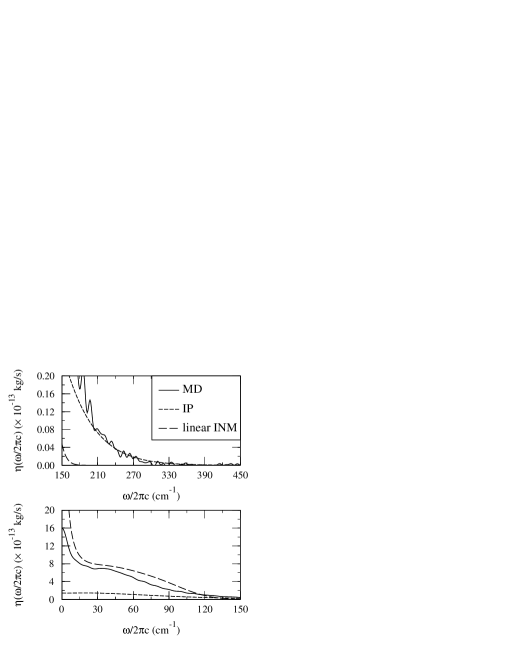
FIG. 1.: The vibrational friction felt by a vibrating diatomic molecule dissolved in a supercritical atomic liquid. Shown here are a number of different calculations for the real part of the frequency–domain vibrational friction of the Tuckerman–Berne model system (under the standard model conditions of reduced density $\rho\sigma_{vv}^{3}=1.05$ and reduced temperature $k_{B}T/\epsilon_{vv}=2.5$) in units appropriate to a Xe solvent. The lower panel is the friction relevant to diatomic whose vibrational frequency falls within the expected bandwidth of the solvent; the upper panel portrays the friction for frequencies above the band edge. (Note the rather different scales used in the two panels.) In both panels, the rough solid line results from an exact molecular dynamics calculation of the bond–force autocorrelation function, the long dashed line (visible only in the lower left hand corner in the upper panel) shows the analogous predictions from linearized instantaneous–normal–mode theory, and the short dashed line gives the analogous predictions from full instantaneous–pair theory.

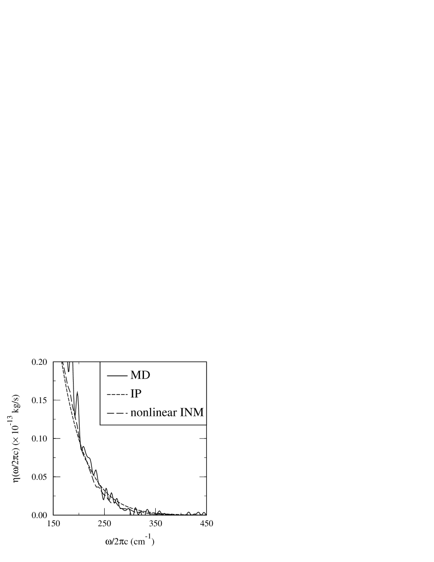
FIG. 2.: The vibrational friction felt by a high-frequency vibrating diatomic molecule dissolved in a supercritical atomic liquid. As in the upper panel of Fig. 1, the calculations are performed for the standard Tuckerman–Berne model system (under the same thermodynamic conditions) with Xe as the solvent, and the solid and short-dashed lines show the full–molecular–dynamics and the full instantaneous–pair theory results, respectively. Here, however, the long–dashed line represents the outcome of the nonlinearly–coupled instantaneous–normal–mode version of the pair theory. Both pair theories interpret the relaxation as a few–body event in which only the initial conditions are prescribed by the fluid. They differ in that the full instantaneous–pair–theory uses the anharmonic dynamics of the key atoms to drive the evolution of the nonlinear solute–solvent coupling, whereas the INM equivalent assumes harmonic dynamics drives this coupling. In contrast to both of these treatments, the linear INM theory of Fig. 1 limits itself to linear coupling.

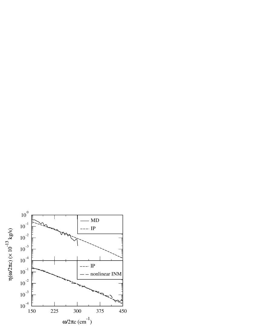
FIG. 3.: The vibrational friction felt by a high–frequency vibrating diatomic molecule dissolved in supercritical atomic Xe. In the upper panel, the instantaneous–pair (short dashes) and molecular dynamics (solid line) results from Fig. 2 are replotted here on a semilog scale to emphasize the near exponential–gap–law behavior. The lower panel compares the instantaneous–pair theory of the upper panel to the analytical results, Eqs. (77), (82), and (84), where to generate $t_{0}$ we have used the value of $\alpha_{0}$ found by averaging over initial mnn distances. For the supercritical fluid, this average $\alpha_{0}$ is $17.2\ \sigma_{Xe}^{-1}\ =\ 4.2\ \AA^{-1}$, which yields a characteristic timescale, $t_{0}\ =\ 0.042\ \tau_{LJ}\ =\ 146fs$. Numerical noise clearly makes it difficult to follow the exact molecular dynamics results over more than a limited frequency interval. It is only by going beyond this interval, however, that the small deviations from strictly exponential behavior begin to manifest themselves in the form of a slight downward curvature to the predictions of the pair theories.

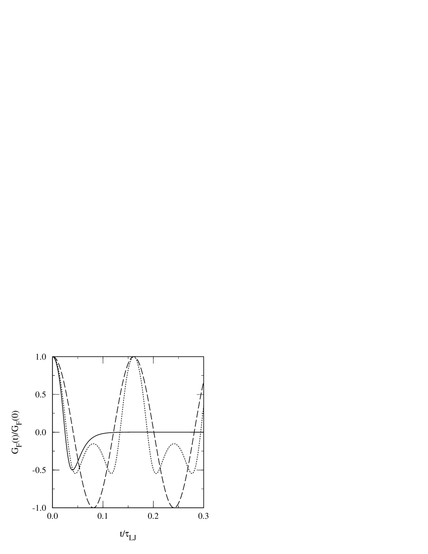
FIG. 4.: The bond–force–velocity autocorrelation function for the standard Tuckerman–Berne model system evaluated at a single initial liquid configuration for three different pair theories. Shown here is a normalized version of the instantaneous correlation function appearing in Eq. (51), $<u^{\prime\prime}[r(t)]\ u^{\prime\prime}[r(0)]\cos^{2}\theta_{0}\ {\dot{r}}(t){\dot{r}}(0)>_{{\bf r_{0}}}$, with the initial displacement between the key solute and solvent atoms held fixed at $r_{0}=|{\bf r_{0}}|=0.95\sigma_{uv}$ and $\theta_{0}=0$. As in Figs. 1–3, the reduced temperature $k_{B}T/\epsilon_{vv}=2.5$. The solid and dotted lines both make use of the manifestly nonlinear solute–solvent Lennard–Jones potential $u(r)$ in evaluating $u^{\prime\prime}(r)$, but they take the time evolution to be given by the anharmonic dynamics of Eq. (54) and the harmonic dynamics of Eq. (56) respectively. The long dashed curve results from the corresponding linear INM theory: that is, from employing both the harmonic dynamics and the linear coupling assumption $u^{\prime\prime}[r(t)]\ \approx\ u^{\prime\prime}[r(0)]$. For Xe, a time interval of $0.1\ \tau_{LJ}$ corresponds to about 350 fs.

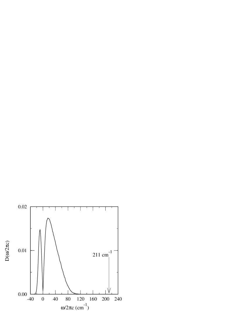
FIG. 5.: The instantaneous–normal–mode density of states for liquid Xe at a density $\rho=3.0g/ml$ and temperature $T=280K$ (computed by taking Xe to be a Lennard–Jones liquid at reduced density and temperature $\rho\sigma^{3}=0.95$ and $k_{B}T/\epsilon=1.26$). Shown by the arrow, for comparison, is the vibrational frequency of I₂ in its ground vibronic state.

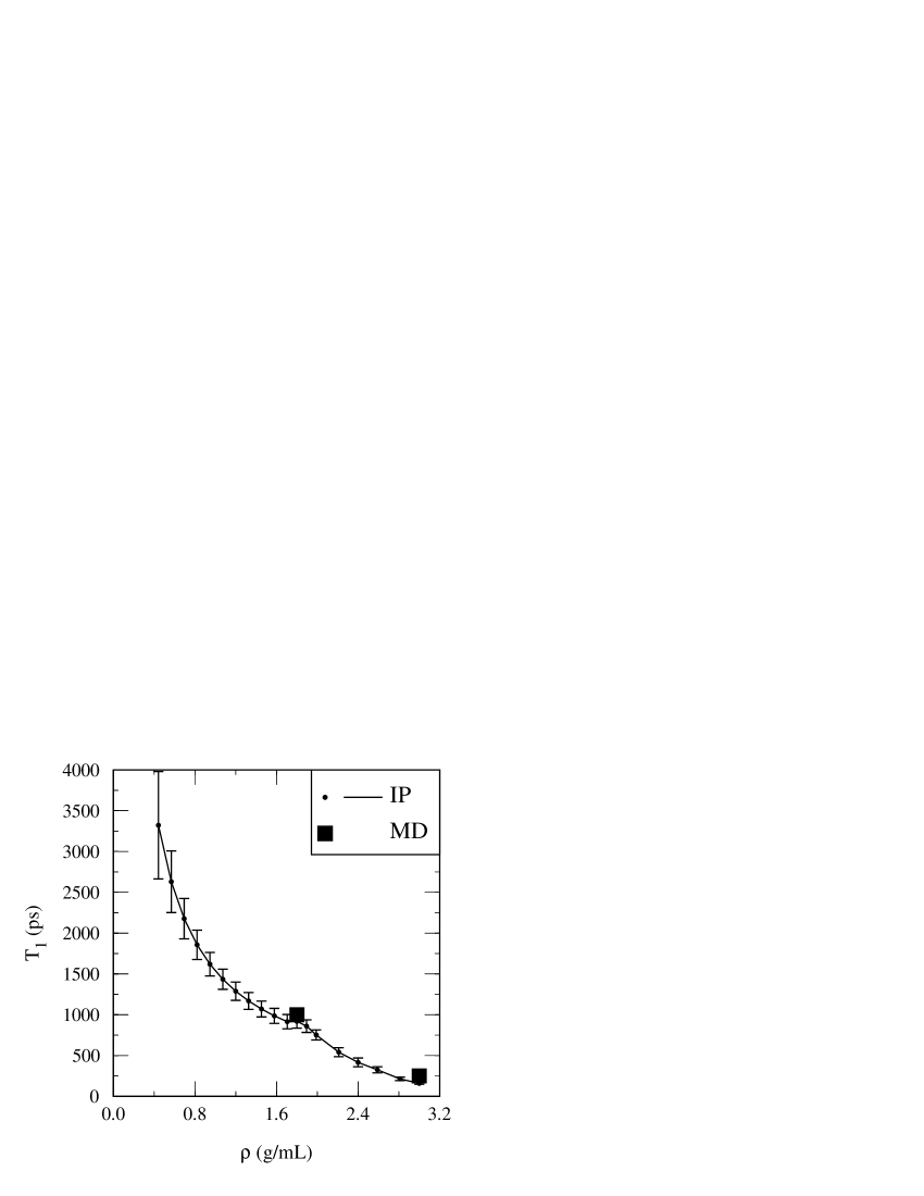
FIG. 6.: Predicted vibrational population relaxation times, $T_{1}$, as a function of liquid density, $\rho$, for I₂ dissolved in liquid Xe at 280 K. Results from the full instantaneous–pair–theory are indicated by dots with a line connecting them drawn to guide the eye. These values were obtained by averaging the instantaneous results over 100,000 liquid configurations for densities less than 2.0 g/mL, 50,000 configurations for $\rho$ = 2.2 g/mL, and 20,000 configurations for all higher densities; 2 standard–deviation error bars are shown. The point indicated by squares are from the full molecular dynamics simulation results of Brown, Harris, and Tully (Ref. [70]) as reported by Harris, Smith, and Russell (Ref. [10]).

REFERENCES

- [1] J. T. Hynes, in Theory of Chemical Reaction Rates, vol. 4, ed. M. Baer (CRC Press, Boca Raton, 1985).
- [2] An experimental example in which the transfer of energy from a solvent into a solute is monitored as a function of time is described in: A. Tokmakoff, B. Sauter, A. S. Kwok, and M. D. Fayer, Chem. Phys. Lett. 221, 412 (1994).
- [3] E. Pollak, in Dynamics of Molecules and Chemical Reactions, ed. R. E. Wyatt, J. Z. H. Zhang (Marcel Dekker, New York, 1996).
- [4] D. D. Dlott, in Laser Spectroscopy in Solids II, W. Yen, ed. (Springer-Verlag, Berlin, 1989).
- [5] S. A. Egorov and J. L. Skinner, J. Chem. Phys. 103, 1533 (1995).
- [6] S. A. Egorov and J. L. Skinner, J. Chem. Phys. 105, 10153 (1995).
- [7] S. A. Egorov and J. L. Skinner, J. Chem. Phys. 106, 1034 (1997).
- [8] H. K. Shin, in Dynamics of Molecular Collisions, part A, ed. W. H. Miller (Plenum Press, N.Y., 1976); Atom-Molecule Collision Theory: A Guide for the Experimentalist, ed. R. B. Bernstein (Plenum, N.Y., 1979).
- [9] J. J. Owrutsky, D. Raftery, and R. M. Hochstrasser, Annu. Rev. Phys. Chem. 45, 519 (1994).
- [10] C. B. Harris, D. E. Smith, and D. J. Russell, Chem. Rev. 90, 481 (1990).
- [11] J. Chesnoy and G. M. Gale, Adv. Chem. Phys. 70 (part 2), 297 (1988).
- [12] B. J. Berne, M. E. Tuckerman, J. E. Straub, and A. L. R. Bug, J. Chem. Phys. 93, 5084 (1990).
- [13] M. E. Tuckerman and B. J. Berne, J. Chem. Phys. 98, 7301 (1993).
- [14] R. M. Whitnell, K. R. Wilson, and J. T. Hynes, J. Phys. Chem. 94, 8625 (1990); J. Chem. Phys. 96, 5354 (1992).
- [15] M. Bruehl and J. T. Hynes, Chem. Phys. 175, 205 (1993).
- [16] R. Rey and J. T. Hynes, J. Chem. Phys. 104, 2356 (1996).
- [17] S. A. Egorov and J. L. Skinner, J. Chem. Phys. 105, 7047 (1996); K. F. Everitt, S. A. Egorov, and J. L. Skinner (preprint).
- [18] S. A. Adelman, R. Ravi, R. Muralidhar, and R. H. Stote, Adv. Chem. Phys. 84, 73 (1993).
- [19] D. W. Miller and S. A. Adelman, Int. Revs. Phys. Chem. 13, 359 (1994).
- [20] A. Tokmakoff and M. D. Fayer, Accts. Chem. Res. 28, 437 (1995); J. Chem. Phys. 103, 2810 (1995).
- [21] S. Gnanakaran and R. M. Hochstrassser, J. Chem. Phys. 105, 3486 (1996); S. Gnanakaran, M. Lim, N. Pugliano, M. Volk, and R. M. Hochstrassser, J. Phys. Condens. Matter 8, 9201 (1996).
- [22] P. Hamm, M. Lim, and R. M. Hochstrasser, J. Chem. Phys. 107, 10523 (1997); R. Rey and J. T. Hynes, ibid. 108, 142 (1998).
- [23] D. W. Oxtoby, Adv. Chem. Phys. 47 (part II), 487 (1981).
- [24] The most accurate results are usually obtained by taking to be the solution–phase value of the vibrational frequency rather than the isolated–molecule value, technically, a renormalized perturbation theory result.
- [25] Typically (though not always) we expect the solute’s vibrations to behave quantum mechanically while the solvent acts largely classically. Quantum corrections computed from semiclassical pictures of this sort have been explored in some depth in the literature. Within some semiclassical models, the resulting quantum mechanical relaxation rates are proportional to (or even equal to) the fully classical result, despite the rather high values of (. See, for example: J. S. Bader and B. J. Berne, J. Chem. Phys. 100, 8359 (1994); S. A. Egorov and B. J. Berne, ibid. 107, 6050 (1997); J. L. Skinner, ibid. 107, 8717 (1997);. We shall focus in this paper on the portion of the problem that is determined by the purely classical behavior.
- [26] J. M. Deutch and R. Silbey, Phys. Rev. A 3, 2049 (1971); R. Zwanzig, J. Stat. Phys. 9, 215 (1973); E. Pollak, J. Chem. Phys. 85, 865 (1986); B. J. Gertner, K. R. Wilson, and J. T. Hynes, J. Chem. Phys. 90, 3537 (1989).
- [27] A. M. Levine, M. Shapiro, and E. Pollak, J. Chem. Phys. 88, 1959 (1988); Yu. I. Georgievskii and A. A. Stuchebrukov, J. Chem. Phys. 93, 6699 (1990).
- [28] G. Goodyear, R. E. Larsen, and R. M. Stratt, Phys. Rev. Lett. 76, 243 (1996).
- [29] G. Goodyear and R. M. Stratt, J. Chem. Phys. 105, 10050 (1996).
- [30] G. Goodyear and R. M. Stratt, J. Chem. Phys. 107, 3098 (1997).
- [31] R. E. Larsen, E. F. David, G. Goodyear, and R. M. Stratt, J. Chem. Phys. 107, 524 (1997).
- [32] B. M. Ladanyi and R. M. Stratt, J. Phys. Chem. 102, 1068 (1998).
- [33] T. Kalbfleisch and T. Keyes, J. Chem. Phys. 108, 7375 (1998).
- [34] S. J. Schvaneveldt and R. F. Loring, J. Chem. Phys. 102, 2326 (1995); 104, 4736 (1996); J. Phys. Chem. 100, 10355 (1996).
- [35] G. Gershinsky and E. Pollak, J. Chem. Phys. 101, 7174 (1994); 103, 8501 (1995); J. Cao and G. A. Voth, ibid. 103, 4211 (1995).
- [36] In two speculative but interesting papers, the authors described some of the results one might someday obtain for the vibrational relaxation of polyatomic molecules in liquids if instantaneous normal modes could actually function as solid–state–like phonons. Although they presented no evidence for their supposition at the time, we show in this paper that their suggestion that one can get multiple-phonon contributions to liquid–state relaxation is, in fact, a correct one. V. M. Kenkre, A. Tokmakoff, and M. D. Fayer, J. Chem. Phys. 101, 10618 (1994); P. Moore, A. Tokmakoff, T. Keyes, and M. D. Fayer, J. Chem. Phys. 103, 3325 (1995).
- [37] The theorem is that (within this model) a solute oscillator of frequency cannot release its energy directly to the solvent unless there are solvent oscillators of frequency . However, we should point out that polyatomic molecules often relax by transferring a significant fraction of their excess vibrational quanta to one or more intramolecular modes of lower frequency, leaving only a lesser amount of vibrational energy to be absorbed by the solvent. See, for example, X. Hong, S. Chen, D. D. Dlott, J. Phys. Chem. 99, 9102 (1995) and Refs. [36] and [16]. Nonetheless, even this smaller quantity of energy will often be well beyond the putative band edge of the solvent.
- [38] D. Rostkier–Edelstein, P. Graf, and A. Nitzan, J. Chem. Phys. 107, 10470 (1997).
- [39] R. M. Stratt, Acc. Chem. Res. 28, 201 (1995).
- [40] B. M. Ladanyi and R. M. Stratt, J. Phys. Chem. 100, 1266 (1996).
- [41] P. Moore and T. Keyes, J. Chem. Phys. 100, 6709 (1994).
- [42] A. Rahman, M. Mandell, and J. P. McTague, J. Chem. Phys. 64, 1564 (1976); P. A. Madden, in Liquids, Freezing, and the Glass Transition, ed. J. P. Hansen, D. Levesque, and J. Zinn–Justin (North–Holland, Amsterdam, 1991).
- [43] Molecular Liquids: Dynamics and Interactions, ed. A. J. Barnes, W. J. Orville-Thomas, and J. Yarwood (D. Reidel, Dordrecht, 1984); Molecular Liquids: New Perspectives in Physics and Chemistry, ed. J. J. C. Teixeira–Dias (Kluwer, Dordrecht, 1992).
- [44] D. McMorrow and W. T. Lotshaw, J. Phys. Chem. 95, 10395 (1991); Chem. Phys. Lett. 201, 369 (1993).
- [45] A. Nitzan, S. Mukamel, and J. Jortner, J. Chem. Phys. 60, 3929 (1974).
- [46] A. Nitzan, S. Mukamel, and J. Jortner, J. Chem. Phys. 63, 200 (1975).
- [47] S. A. Passino, Y. Nagasawa, and G. R. Fleming, J. Chem. Phys. 107, 6094 (1997); T. Steffen and K. Duppen, ibid. 106, 3854 (1997); F. Sciortino and P. Tartaglia, Phys. Rev. Lett. 78, 2385 (1997).
- [48] K. Okumura and Y. Tanimura, J. Chem. Phys. 107, 2267 (1997).
- [49] E. F. David and R. M. Stratt, J. Chem. Phys. 109 (1998) (in press).
- [50] P. K. Davis and I. Oppenheim, J. Chem. Phys. 57, 505 (1972).
- [51] D. Oxtoby, Mol. Phys. 34, 987 (1977).
- [52] J. Chesnoy and J. J. Weis, J. Chem. Phys. 84, 5378 (1986).
- [53] M. E. Paige and C. B. Harris, Chem. Phys. 149, 37 (1990); J. Chem. Phys. 93, 3712 (1990); D. J. Russell and C. B. Harris, Chem. Phys. 183, 325 (1994).
- [54] M. Fixman, J. Chem. Phys. 34, 369 (1961); R. Zwanzig, ibid. 34, 1931 (1961); R. Zwanzig, ibid. 36, 2227 (1962).
- [55] P. S. Dardi and R. I. Cukier, J. Chem. Phys. 89, 4145 (1988); P. S. Dardi and R. I. Cukier, ibid. 95, 98 (1991).
- [56] C. J. S. M. Simpson, M. L. Turnidge, and J. P. Reid, J. Mol. Liq. 70, 125 (1996).
- [57] R. M. Stratt and M. Cho, J. Chem. Phys. 100, 6700 (1994).
- [58] W. A. Steele, Mol. Phys. 61, 1031 (1987).
- [59] In writing the friction in this fashion we have neglected a term proportional to .
- [60] In our examples, two different solvent atoms are mutual nearest neigbors of the two solute atoms in about 30 percent of the liquid configurations. Most of the configurations, about 50 percent, have only a single solvent as a mutual nearest neighbor; the remainder are such that the solute has no solvents as mutual nearest neighbors.
- [61] For any quantity , the classical ensemble average , so on the average we obtain , the mean square angular velocity.
- [62] Typical liquid–state values for the temperature fall between the triple point and the critical point, . Typical mutual-nearest-neighbor distances are actually on the order of in a Lennard–Jones liquid (see, for example, Ref. [31]), which would imply an even larger value of the intermolecular force than we used in our estimate. Indeed, the fact that this small a change in the intermolecular distance leads to a value of the force 3.5 times larger is itself a good illustration why both the coupling and dynamics are dominated by the solvent atoms nearest to the solute atoms.
- [63] It is worth pointing out that in deriving the Eq. (41), we did not need to assume that the intermolecular force was larger than the intramolecular force; the intramolecular forces operating on the two solute sites are necessarily equal and opposite and therefore make no net contribution to the center–of–mass motion.
- [64] For I2 dissolved in Xe, , whereas for a dense Lennard–Jones liquid, the full width at half maximum of the mutual–nearest–neighbor distribution is about .
- [65] M. Buchner, B. M. Ladanyi, and R. M. Stratt, J. Chem. Phys. 97, 8522 (1992).
- [66] Handbook of Mathematical Functions, ed. M. Abramowitz and I. A. Stegun (Dover, New York, 1972), chap. 22.
- [67] The concept of a liquid–state analog to the multiphonon processes seen in solids was also discussed recently by Egorov and Berne (Ref. [25]).
- [68] The analogous resummation for solid–state multiphonon vibrational relaxation is well known. See Refs. [6] and [46]. However we believe the results given here present microscopic evidence that high frequency vibrational relaxation in liquids can be interpreted in a multiphonon language. Indeed, our INM results are somewhat different from the expressions that appear in the solid–state literature, not so much because of the quantum mechanical character of the literature derivations (which give results identical in form to those from a classical derivation), but because of the INM approach’s explicit inclusion of anharmonicity in the distribution of initial conditions.
- [69] Our LJ parameters for xenon are identical to those used in the simulations of Brown, Harris and Tully, Ref. [70].
- [70] J. K. Brown, C. B. Harris, and J. C. Tully, J. Chem. Phys. 89, 6687 (1988).
- [71] M. P. Allen and D. J. Tildesley, Computer Simulation of Liquids (Clarendon Press, Oxford, 1987), Chaps. 1 and 4.
- [72] Allen and Tildesley, Ref. [71], Chap. 3.
- [73] The initial velocities selected, , were averaged as pairs so as to minimize numerical noise.
- [74] In order to facilitate comparisons, the integrator and the time step employed here were the same as that for the full molecular dynamics simulation, velocity–Verlet and , respectively. However since the instantaneous–pair theory requires only a one–dimensional trajectory, it would have been computationally trivial to use a higher order integrator and a far smaller time step had we needed more reliable high–frequency information.
- [75] All Fourier transforms were performed using the FFT algorithm cosft, from W. H. Press, S. A. Teukolsky, W. T. Vetterling, and B. P. Flannery, Numerical Recipes in C, 2nd ed. (Cambridge University, London, 1994).
- [76] See, for example, J. S. Bader, B. J. Berne, E. Pollak, and P. Hänggi, J. Chem. Phys. 104, 1111 (1996).
- [77] The theoretical origins of exponential gap laws governing single–collision vibrational excitations are reviewed in M. S. Child, Molecular Collision Theory (Academic Press, London, 1974), Chaps. 7 and 8. For an example of a similar gap law for rotational excitation, see J. C. Polanyi and K. B. Woodall, J. Chem. Phys. 56, 1563 (1972).
- [78] Inasmuch as we were careful to use the same molecular dynamics integrators and the same size time steps with the pair–theory and with the full molecular dynamics calculation, the pair theory’s superior numerical stability in Figs. 1 and 2 is striking. We attribute the difference to the much higher level of velocity averaging possible with the pair theory.
- [79] The values of turn out to be surprisingly constant, suggesting that even a Lennard–Jones potential looks remarkably exponential insofar as high–frequency dynamics goes. Over the full width at half maximum of the mutual–nearest–neighbor distribution for this thermodynamic state ( – ), the value of for the Lennard–Jones potentials used here.
- [80] Parenthetically, were we to recompute the nonlinearly–coupled/harmonic–dynamics curve with inertial (constant force) dynamics (not shown) instead of harmonic dynamics, sum rules would still generate the correct initial decay for us, but the trajectories would soon wander off into regions of impossibly high potential energy, leaving us with nonsensical correlation functions.
- [81] The densities of liquid and gaseous Xe at coexistence were obtained from the Lennard–Jones phase diagram given by Yu. V. Kalyuzhnyi and P. T. Cummings, Mol. Phys. 87, 1459 (1996).
- [82] G. Herzberg, Infrared and Raman Spectra, (Van Nostrand Reinhold, New York, 1945) pp. 241 and 246.
- [83] Y. Tanimura and S. Mukamel, J. Chem. Phys. 99, 9496 (1993).
- [84] K. Okumura and Y. Tanimura, J. Chem. Phys. 105, 7294 (1996); 106, 1687 (1997); Chem. Phys. Lett. 278, 175 (1997).
- [85] A. Tokmakoff and G. R. Fleming, J. Chem. Phys. 106, 2569 (1997); A. Tokmakoff, M. J. Lang, D. S. Larsen, G. R. Fleming, V. Chernyak, and S. Mukamel, Phys. Rev. Lett. 79, 2702 (1997).
- [86] R. L. Murry and J. T. Fourkas, J. Chem. Phys. 107, 9726 (1997); R. L. Murry, J. T. Fourkas, and T. Keyes (preprint I.); R. L. Murry, J. T. Fourkas, and T. Keyes (preprint II.).
- [87] T. Steffen and K. Duppen, Ref. [47].
- [88] K. Tominaga and K. Yoshihara, Phys. Rev. Lett. 74, 3061 (1995); J. Chem. Phys. 104, 4419 (1996).
- [89] S. Saito and I. Ohmine, J. Chem. Phys. 108, 240 (1998).
- [90] See, for example, the discussion of the intermolecular dynamics of in Ref. [48]. The opposite conclusion seems to be drawn for intramolecular mode couplings in by Okumura and Tanimura (Chem. Phys. Lett., 1997, Ref. [84]), but it is unclear the extent to which the the authors are looking at intramolecular (as opposed to intermolecular) anharmonicity.
- [91] An early forerunner of just such an approach, which featured a quantum mechanical few–body scattering calculation embedded in a many–body theory for vibrational relaxation, is that of H.–Y. Sun and S. A. Rice, J. Chem. Phys. 42, 3826 (1965).
- [92] I. S. Gradshteyn and I. M. Ryzhik, Table of Integrals, Series, and Products, 4th ed. (Academic Press, New York, 1965) p. 338.