Detecting periodicity in experimental data using linear modeling techniques

Abstract

Fourier spectral estimates and, to a lesser extent, the autocorrelation function are the primary tools to detect periodicities in experimental data in the physical and biological sciences. We propose a new method which is more reliable than traditional techniques, and is able to make clear identification of periodic behavior when traditional techniques do not. This technique is based on an information theoretic reduction of linear (autoregressive) models so that only the essential features of an autoregressive model are retained. These models we call reduced autoregressive models (RARM). The essential features of reduced autoregressive models include any periodicity present in the data.

We provide theoretical and numerical evidence from both experimental and artificial data, to demonstrate that this technique will reliably detect periodicities if and only if they are present in the data. There are strong information theoretic arguments to support the statement that RARM detects periodicities if they are present. Surrogate data techniques are used to ensure the converse. Furthermore, our calculations demonstrate that RARM is more robust, more accurate, and more sensitive, than traditional spectral techniques.

I Introduction

Periodic, and nearly periodic, behavior is a common feature of many biological and physical systems and there exist several widely-used techniques to estimate the period of a behavior, for example, spectral estimation [1], autocorrelation [1], spectrographs, band pass (comb) filters [2] and wavelet transforms [3, 4]. All of these standard techniques either employ, or are related to, or are a generalization of, Fourier series.

In this paper we propose an alternative method of detecting periodicity that is not so closely related to Fourier series. This new technique applies ideas from information theory to linear autoregressive models of time series to extract evidence of periods.

The basic principle is the following. Given a time series $\{y_{t}\}_{t=1}^{N}$ one can propose a linear autoregressive model $AR(n)$ by

$$y_{t} = a_{1}y_{t-1}+a_{2}y_{t-2}+a_{3}y_{t-3}+\ldots$$ (2)

$$+a_{n}y_{t-n}+e_{t}\;\;t=n+1,n+2,\ldots,N.$$

where $e_{t}$ are assumed to be independent and identically distributed random variables, which are interpreted as the modeling errors [1, 5]. Under these assumptions the maximum likelihood estimate of the parameters $a_{1},a_{2},\ldots,a_{n}$ can be written in terms of a covariance function, and are therefore related to the autocorrelation function and Fourier spectrum. It is common practice to determine the optimal size $n$ of the model by using either the Akaike [6] or the Schwarz [7] information criteria; this is done to avoid over-fitting of the time series [8]. It has recently been observed that a further optimization of an $AR(n)$ model may be possible by deleting some of the terms to obtain a model

$$y_{t} = a_{0}+a_{1}y_{t-\ell_{1}}+a_{2}y_{t-\ell_{2}}+a_{3}y_{t-\ell_{3}}+\ldots$$ (4)

$$+a_{k}y_{t-\ell_{k}}+e_{t},$$

where,

$\displaystyle 1\leq\ell_{1}<\ell_{2}<\ell_{3}<\ldots<\ell_{k}\leq n$

for $\ell_{i}\in{\rm\bf Z}^{+}\;\;i=1,2,3,\ldots,k$. The hope is to obtain a model that fits the time series equally well, but has far fewer parameters. Profound theoretical arguments, which are a codification of Occam’s razor, imply that if a reduced autoregressive model (RARM) is suitably optimized, then it is superior to an equivalent autoregressive model $AR(n)$. The key principle of this paper is that if one has an optimized RARM, that is the RARM that has been reduced to only the essential terms, then the parameters $\ell_{1},\ell_{2},\ell_{3},\ldots,\ell_{k}$, often called lags, provide information about the periodicity of the time series.

A practical procedure for obtaining an optimal reduced autoregressive model (RARM) has been described by Judd and Mees [9]. This procedure was introduced in the more general context of nonlinear modeling, but in the following section we describe briefly the underlying theory in the context of RARM.

The major part of this paper is aimed at presenting evidence that examining the lags of an optimal RARM provides a more robust and accurate means of detecting periods in time series than traditional spectral techniques. That is, the proposed technique unambiguously identifies periodicities even when spectral methods fail to do so, and furthermore, does not falsely suggest the presence of periods when none are present. The evidence presented is a combination of theoretical argument and numerical procedures, which are illustrated with both artificial and experimental data.

An important numerical procedure that will be used to establish that the proposed technique does not falsely identify periods is surrogate data analysis. The principle of surrogate data analysis is the following. From experimental data one generates artificial data that are “similar” to the experimental data and satisfy a given hypothesis. One then calculates a test statistic for each surrogate data set, and hence obtains an ensemble of statistic values that estimate the distribution of the test statistic under the assumption that the original data is consistent with the given hypothesis. One then compares the statistic value of the original data with the estimated distribution of the surrogates. If the data has an atypical statistic value then the hypothesis will be rejected, otherwise it should be accepted. In this paper we employ this technique to ensure that RARM procedures do not spuriously identify periodicities in temporally uncorrelated surrogate data.

A Minimum description length

The criteria we use for determining the optimal RARM is the minimum description length. Occam’s razor recommends that the best description of a phenomenon is the shortest description. This principle can be made rigorous using information theory, and the principle was independently developed by Wallace [10] and Rissanen [11].

Operationally the principle is applied as follows. Suppose you have a time series $\{y_{t}\}_{t=1}^{N}$ given to a certain fixed accuracy and that you wish to communicate the data to a colleague. To send the raw data would require a certain number of bits. Alternatively, one could build a predictive model, of the form (4) for example, and then send the model parameters (to some precision), the initial $\ell_{k}$ observations, and the differences between the model’s predictions and actual observations. Given this information your colleague can reconstruct the original data. If the model of the time series is good, then the total number of bits required for parameters, initial conditions and prediction errors is less than the number of bits of raw data, because the differences between the predicted and actual observations are smaller than the observations. The total number of bits sent in the second case is called the description length, and the model that achieves the minimum description length is the one recommended by the application of Occam’s razor. The dogma is that this model achieves the best prediction of the data without over-fitting.

In practice it is usually sufficient to estimate the description length of a model, rather than calculate it in detail. An estimate will usually have the form

$$\left(\mbox{description length}\right)\approx(\mbox{number of data})$$

$$\hskip 14.22636pt\times\log\left(\mbox{sum of squares of prediction errors}\right)$$

$$\hskip 14.22636pt+\left(\mbox{penalty for number and accuracy of parameters}\right).$$

Following Judd and Mees [9] the description length of a RARM can be estimated as follows. Given a time series $\{y_{t}\}_{t=1}^{N}$ define a set of vectors $\{V_{i}\}_{i=1}^{n}$ by

$\displaystyle V_{0}=(1,1,\ldots,1)^{T},$

$\displaystyle V_{1}=(y_{n},\ldots,y_{N-1})^{T},$

$\displaystyle V_{2}=(y_{n-1},\ldots,y_{N-2})^{T},$

$\displaystyle\vdots$

$\displaystyle V_{j}=(y_{n-j+1},\ldots,y_{N-j})^{T},$

$\displaystyle\vdots$

$\displaystyle V_{n}=(y_{1},\ldots,y_{N-n})^{T},$

and define

$\displaystyle y=(y_{n+1},\ldots,y_{N})^{T}.$

Observe that if the model (4) is appropriate for the time series one can write

$$y=\sum_{i=1}^{k}a_{i}V_{\ell_{i}}+e$$ (5)

$\displaystyle=V_{B}a_{B}+e,$

where $B=(\ell_{1},\ell_{2},\ldots,\ell_{k})$, $V_{B}=[V_{\ell_{1}}|V_{\ell_{2}}|\cdots|V_{\ell_{k}}]$ is a matrix, and $a_{B}=(a_{1},a_{2},\ldots,a_{k})^{T}$. The maximum likelihood estimates of $a_{B}$, that is, the values that minimize $e^{T}e$, are given by

$\displaystyle a_{B}=(V_{B}^{T}V_{B})^{-1}V_{B}^{T}y.$

Now each parameter $a_{j}$ must be sent to some precision $\delta_{j}$, that is, the maximum likelihood estimate of $a_{j}$ is “rounded-off” by an amount $\delta_{j}$. It can be shown [9] that the optimal precisions $\delta=(\delta_{1},\delta_{2},\ldots,\delta_{k})$, that is, the round-off for each $a_{j}$ that gives the minimum description length, satisfy

$\displaystyle(Q\delta)_{j}=1/\delta_{j}$

where

$\displaystyle Q=\frac{-NV_{B}^{T}V_{B}}{(a_{B}V_{B}-y)^{T}(a_{B}V_{B}-y)}.$

Consequently, it can be shown [9] that the approximate description length of the RARM (4) is

$$\frac{N}{2}\left(1+\ln{\frac{2\pi e^{T}e}{N}}\right)+\left(\frac{1}{2}+\ln\gamma\right)k-\sum_{j=1}^{k}\ln\delta_{j},$$ (6)

where $\gamma$ is a constant depending on the overall scale of the data.

Armed with this estimate of the description length of a RARM one can search over all combinations of lags $B=(\ell_{1},\ell_{2},\ldots,\ell_{k})$ to obtain the optimal RARM, however, Judd and Mees [9] describe a fast and efficient method of doing this optimization.

II Detecting periodicity using optimal RARM

A function $f$ is periodic with period $\tau$ if $f(t)=f(t+\tau)$ for all $t$. A time series (assumed stationary) has an (approximate) periodicity of period $\tau$ if $y_{t}\approx y_{t+\tau}$ for all $t$, or, equivalently, the autocorrelation $\rho$ has a local maximum at $\tau$. The reduced autoregressive model (4) predicts the current value of a time series $y_{t}$ as a weighted average of the previous values, that is, at the time steps $\ell_{1}$, $\ell_{2}$, $\ldots$, and $\ell_{k}$ previous to $t$. If a time series has periodic behavior, then the lags $\ell_{1},\ell_{2},\ldots,\ell_{k}$ should be (multiples of) the periods.

We claim that one can detect in time series a periodicity of period $\leq{}n_{MAX}$ by the following procedure, called the RARM procedure. For $n=0,1,2,3,\ldots,n_{MAX}$ build optimal reduced autoregressive models of the form (4) using the algorithm described by Judd and Mees [9]. For each model in this sequence calculate its description length (6) and take as the overall optimal model that model with the smallest description length. We claim that if the overall optimal RARM is non-trivial, then the lags $\ell_{1},\ell_{2},\ldots,\ell_{k}$ should be (multiples of) the periods $\leq{}n_{MAX}$ in the original time series if the time series is sufficient long.

In order to establish our claim we must demonstrate that

1. if the time series contains a period then the RARM procedure detects this periodic behavior, and

2. if the RARM procedure detects a period then there is periodic behavior in the time series.

In section II A we provide a theoretical argument to establish the forward implication (i). In section II B we discuss an essential procedure for ensuring (ii).

A Forward implication (i)

The argument to establish the forward implication proceeds as follows. First, we observe that a period in a time series will (regardless of whether it is linear or nonlinear) produce a local maximum in the autocorrelation function $\rho(\tau)$. Next it is shown below that, in the optimization of a RARM of given maximum size $n$, the criterion for inclusion of a particular term $a_{j}y_{t-\ell_{j}}$ in (4) is closely related to the magnitude of the autocorrelation at $\ell_{j}$, $\rho(\ell_{j})$. Hence, if $n$ is large enough, the optimal RARM will include a term corresponding to this periodicity. Rissanen’s minimum description length criterion guarantees that provided the time series is sufficiently long this will always be the case and so the RARM procedure will always detect periods that are present in a time series, provided the time series is sufficiently long.

The remainder of this section elaborates on the detail of this argument. A period $\tau$ in a time series $\{y_{t}\}_{t=1}^{N}$ of $N$ scalar measurements is a strong positive correlation between values separated by $\tau$ time steps, i.e. the autocorrelation

$$\rho(\tau)=\frac{(y-\overline{y})^{T}(V_{\tau}-\overline{y})}{\sum_{n+1}^{N}(y-\overline{y})^{2}}$$ (7)

has a local maximum at $\tau$. Without loss of generality we may assume that $\overline{y}=0$, and therefore (7) reduces to

$$\rho{(\tau)}=\frac{V_{\tau}^{T}y}{y^{T}y}.$$ (8)

Let the set of lags for the optimal RARM of size $k$ be denoted by $B_{k}=(\ell_{1}^{(k)},\ell_{2}^{(k)},\ldots,\ell_{k}^{(k)})$. The vector $B_{k}$ uniquely determines the least squares model

$\displaystyle y=\sum_{i=1}^{k}a^{(k)}_{i}V_{\ell_{i}^{(k)}}+e.$

Define

$$L(\tau) = \left|V_{\tau}^{T}y-\sum_{i=1}^{k}a^{(k)}_{i}V_{\tau}^{T}V_{\ell_{i}^{(k)}}\right|$$ (9)

$$= y^{T}y\left|\rho(\tau)-\sum_{i=1}^{k}a^{(k)}_{i}\rho(\tau-\ell_{i}^{(k)})\right|$$ (10)

According to the algorithm of Judd and Mees [9], given $B_{k}$ and $a^{(k)}_{B}$, the next best term to add to the model has the lag $\tau$ that maximizes $L(\tau)$. However, identity (10) implies that such a $\tau$ is a local maximum of $\rho(\tau)$.

Rissanen’s minimum description length ensures that, for sufficiently large $N$, “if there is any machinery behind the data, which restricts the future observation in a similar manner as the past and which can be captured by the selected class of parametric functions, then we will find that machinery” [11]. The argument in the preceding paragraphs demonstrates that RARM are a sufficiently broad class of parametric functions to capture “machinery” behind the data, including observed periodicities. Thus, if periodicity is present in the data then RARM techniques will detect it — provided $N$ is sufficiently large. This ensures the forward implication (i).

B Reverse implication (ii): Surrogate data techniques

In order to establish that the RARM techniques does not falsely identify a period when none is present, the numerical procedure of surrogate data analysis can be used. The technique of surrogate data was originally introduced by Theiler and colleagues [12]. They suggest three surrogate generation techniques to address three different hypotheses about a time series, but for our purposes we only use Theiler’s algorithm $0$ surrogates.

In the present case we are interested in whether a time series contains periodicities, or said in another way, we wish to test the null hypothesis that the time series contains no periodicities, that is, has no temporal correlation. Theiler’s algorithm $0$ generates surrogate time series having no temporal correlation by simply shuffling the original time series, or put another way, the surrogates are i.i.d. noise having the same same rank distribution as the original time series [13].

Our proposal is to use optimal RARM as the test for periodicity, that is, if the optimal RARM is non-trivial in that $k>0$ in (4), then periods are present in the time series. To believe the validity of this test one must require that if the optimal RARM detects a period in a time series, then it must not detect any period in algorithm $0$ surrogates [13, 14]. This surrogate test must be applied to each data set for which an optimal RARM has been constructed to ensure that the structure detected in each data set is genuine. That is, we propose that an algorithm $0$ surrogate test is a necessary part of the procedure of detecting periodicity using an optimal RARM. If RARM methods identify periodicity in the surrogates then this is clear evidence of false identification of periodicity in the data. However, if the RARM algorithm detects no periodicity in the surrogates then periodicity identified in the original data is genuine. To ensure the reverse implication (ii) holds one need only apply an algorithm $0$ surrogate calculation.

III Calculations

In this section we demonstrate with artificial and experimental data that RARM detects periodic behavior (i) if and (ii) only if it is present in the original time series. To demonstrate that RARM detects periodic behavior if it is present in the data we construct artificial data contaminated with noise and demonstrate the effectiveness of the RARM algorithm. We compare the RARM results to traditional Fourier spectral and autocorrelation techniques. We repeat these calculations for some experimental data comparing the RARM algorithm and traditional techniques. To demonstrate that our RARM algorithm detects periodic behavior only if it is present in the data we apply the method of surrogate data.

In section III A we describe the application of these techniques to detect periodicities in recordings of infant respiratory patterns during natural sleep. Section III B applies these methods to artificial data sets to demonstrate the effectiveness of these techniques compared to traditional methods. Section III C describes the application of these same methods to global climatic data.

A Infant respiratory data

Using inductance plethysmography we have collected measurements of cross-sectional area of the abdomen of infants during natural sleep. From these measurements we extract a measure that can be related to the breath volume [15]. Figure 1 gives an example of data collected in this way.

We applied our RARM procedure to the data illustrated in figure 1 and obtained a model of the form

$$y_{t}=a_{0}+a_{1}y_{t-1}+a_{2}y_{t-6}+e_{t}$$ (11)

where $a_{0}\approx 2.945206$, $a_{1}\approx 0.300739$ and $a_{2}\approx 0.202056$. Figure 2 shows the result of analysis of this data set with a fast Fourier transform algorithm (MATLAB’s spectrum command.) and an estimate of the autocorrelation function. Both these techniques yield small peaks at the same value (that is, $6$) and are consistent with the results of our RARM algorithm. However, the results are not as unambiguous as the results of the RARM algorithm. That is, the RARM detects a periodicity that is not strong enough to be unambiguously identified by spectral methods.

For many time series of breath size [16] we have computed autocorrelation and Fourier spectral estimates. We have applied our RARM algorithm to each data set and compared this to the result of applying traditional techniques. For these data the period of periodic behavior detected by the RARM algorithm is consistent with the periods detected by autocorrelation. That is, if RARM detects periodic behavior, then it is of the same period as that detected by the autocorrelation estimate (if the autocorrelation detects periodic behavior). Furthermore, if RARM does not detect periodic behavior, then neither does the autocorrelation estimate. The traditional techniques will often fail to detect periodic behavior when the RARM algorithm does detect it.

We have provided experimental evidence that the RARM technique detects periodic behavior when it does occur. Now we will demonstrate that the RARM technique does not lead to spurious identification of periodic behavior. That is, we will show that if the RARM algorithm detects periodic behavior, then there is periodic behavior in the data. To do this we apply a surrogate data algorithm which will ensure that false indications of periodicities can always be identified.

For the data illustrated in figure 1, none of $100$ surrogates generated by shuffling the data exhibited periodic behavior of any period. This calculation was repeated with another $48$ data sets [16]. In all $49$ cases the RARM failed to detect periodic behavior in the surrogate data in at least $99$ (of $100$) surrogates of each data set. This indicates that the RARM algorithm does not identify periodicities not present in the data.

B Artificial data

In this section we use the optimal RARM from section III A as a basis for generating noisy artificial data with a known periodicity. From (11) we use the model

$$y_{t}=a_{0}+a_{1}y_{t-1}+a_{2}y_{t-6}+e_{t}$$ (12)

(where $a_{0}\approx 2.945206$, $a_{1}\approx 0.300739$ and $a_{2}\approx 0.202056$, as above) to generate an artificial data set $y$. To this data we add observational noise $\epsilon_{t}$ and apply the above analysis to the series $z$, $z_{t}=y_{t}+\epsilon_{t}$. Figure 3 demonstrates the result of this technique for an artificial data set of the same length as the data and normal observational noise with standard deviation $1$ ($e_{t},\epsilon_{t}\sim N(0,1)$). Figure 4 is the result of the same technique for a longer data set ($5000$ data points) and more observational noise ($e_{t}\sim N(0,1)$ and $\epsilon_{t}\sim N(0,2)$). In both cases RARM clearly identified periodic behavior with period $6$. For the time series in shown in figures 3 and 4 we constructed $100$ algorithm $0$ surrogates. none of them exhibited periodicity detected by RARM.

The traditional Fourier spectral and autocorrelation techniques identify the same period as the RARM technique for the shorter, but less noisy data illustrated in figure 3. However, for the data shown in figure 4 the RARM technique has identified periodicities that are not obvious from traditional techniques. Furthermore, it should be noted that in all cases that the results of the autocorrelation and spectral methods are not clear cut. For reasonably long, but extremely noisy data sets the RARM algorithm still provides a decisive and accurate estimate of the period of periodic behavior present in data.

C Global climatic data

In this section we describe the application of these techniques with noisy physical data. The time series we use here is monthly deviations from monthly mean global air temperatures over the period 1856–1997 [17]. These global air temperature measurements are obtained by averaging observations at many spatially separated sites on the globe. Figure 5 shows the complete data set. A more detailed discussion of this data may be found in [18]. Analysis using the methods described in this paper demonstrates the presence of periodic fluctuation over periods of $7$ months, $2$ years and $45$ months[19]. Fourier spectral and autocorrelation estimates were also applied (after de-trending this time series) and the results are illustrated in figure 5. From $100$ algorithm $0$ surrogates RARM did not detect periodicity in $99$ of them. These results demonstrate the presence of genuine periodic fluctuation in this time series and that the fluctuation is difficult to detect with traditional techniques. An advantage of the RARM technique is that no de-trending is required. The results of the RARM algorithm are not effected by trends or non-stationarity.

IV Conclusions

We have provided theoretical and experimental evidence to support the use of RARM techniques to detect periodic behavior in noisy experimental time series. The concept of minimum description length ensures that a RARM built with an MDL modeling criterion will detect any periodicities present in the data. We provided numerical evidence using experimental and artificial data to support this. Moreover these calculations have demonstrated that the RARM algorithm provides an accurate and decisive method of detecting periodicities that is more sensitive than Fourier spectrum or autocorrelation methods.

By applying surrogate data techniques we have demonstrated that the RARM algorithm did not identify periodicities in temporally uncorrelated surrogates. This is strong experimental evidence that the RARM algorithm is robust against identification of false periodicities. It does not identify behavior not present in the original system. However this result has only been supported by numerical evidence and does not imply that true identification with arbitrary data. To guard against false positives we recommend application of surrogate data tests, as discussed in this paper. Periodicity detected using RARM are genuine provided RARM detects no periodicity in i.i.d. surrogates.

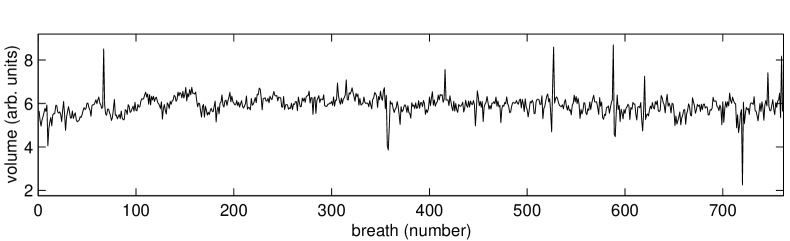
FIG. 1.: Tidal volume: The horizontal axis is breath number — each datum in this time series corresponds to a single breath. The vertical axis is derived from the output from the analogue to digital converter (proportional to cross-sectional area measured by inductance plethysmography, arbitrary units). For each breath the minimum and maximum value over that breath were calculated and the difference recorded. This data set consists of $762$ points recorded from a $21$ week old male during $24$ minutes of continuous stage $2$ sleep. This study had approval from the ethics committee of Princess Margaret Hospital. The parents of this subject were informed of the procedure, and its purpose, and had given consent. The recording took place during a scheduled overnight sleep study at Princess Margaret Hospital.

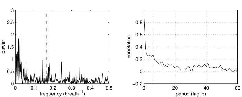
FIG. 2.: Spectral techniques: Estimates of the power spectrum (arbitrary units) and autocorrelation function for the data illustrated in figure 1. The RARM detected periodic motion over a period of $6$ data points, see equation (11). A vertical dot-dashed line marks the location of period 6 behavior in both the frequency (power spectrum) and time (autocorrelation) domain. A peak in the autocorrelation function corresponds exactly with the period $6$ behavior detected by RARM. The power spectrum has a peak close to a frequency of $6^{-1}\approx 0.166667$. A period of $6$ is the closest integer value to the peak evident at this location in the power spectrum. Whilst both power spectra and autocorrelation detect behavior with a period of $6$ these results are not as conclusive as the RARM algorithm.

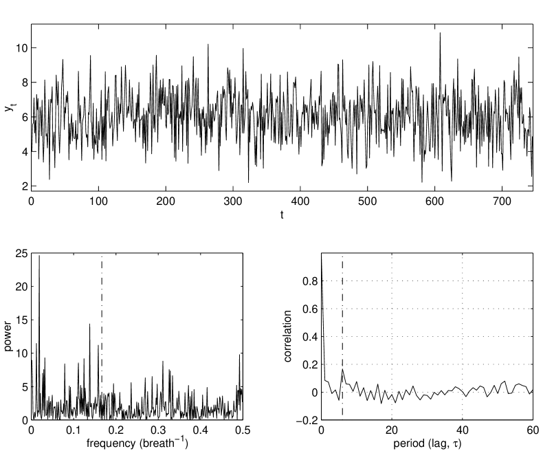
FIG. 3.: Artificial data: A data set of $764$ realization of the process described by (12) with normal observational noise, standard deviation 1. This linear model is of the same form as that predicted from the model of the data in figure 1. Also shown in the power spectrum (arbitrary units) and autocorrelation estimate for this data set. For this data set RARM gave a clear indication of period $6$ behavior. The dot dashed line on the power spectrum and autocorrelation function corresponds to the period of $6$ detected by RARM.

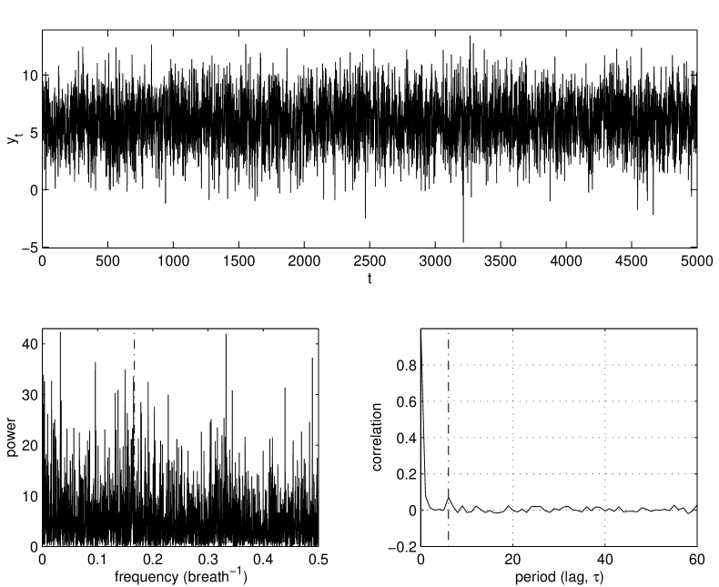
FIG. 4.: Artificial data: Data from an reduced autoregressive of the same form as that predicted from the model of the data in figure 1. This data sets consists of $5000$ realizations of (12) with observational noise, standard deviation 2. Also shown in the power spectrum (arbitrary units) and autocorrelation estimate for this data set. For this data set RARM gave a clear indication of period $6$ behavior. The dot dashed line on the power spectrum and autocorrelation function corresponds to the period of $6$ detected by RARM.

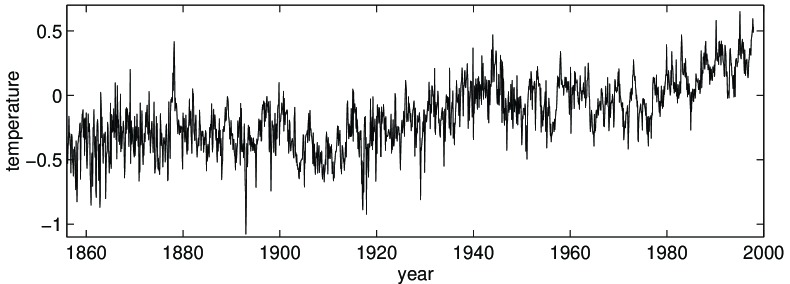
FIG. 5.: Global air temperature: Monthly global air temperature measured as deviation (in degrees Celsius) from monthly mean temperature for the period 1856-1997 ($1704$ data).

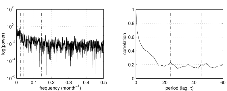
FIG. 6.: Spectral techniques: Estimates of the power spectrum and autocorrelation function for the data illustrated in figure 5. The data in figure 5 was linearly de-trended before calculating Fourier spectrum and autocorrelation. The RARM detected periodic motion over a period of $7$, $24$ and $45$ months. A vertical dot-dashed line marks the location of period $7$, $24$ and $45$ behavior in both the frequency and time domain. A peak in the autocorrelation function corresponds exactly with the period $24$ and $45$ behavior detected by RARM. The power spectrum has a peak close to a frequency of $45^{-1}\approx 0.0222$. Whilst both power spectra and autocorrelation detect behavior with a period of $24$ and $45$ these results are not as conclusive as the RARM algorithm.

REFERENCES

- [1] M. B. Priestly, Non-linear and non-stationary time series analysis (Academic Press, London, 1989).
- [2] P. J. Brusil, T. B. Waggener, R. E. Kronauer, and J. Philip Gulesian, J Appl Physiol 48, 545 (1980).
- [3] C. S. Burrus, R. A. Gopinath, and H. Guo, Introduction to wavelets and wavelet transforms: a primer (Prentice Hall, Upper Saddle River, N.J., 1998).
- [4] Wavelet theory and harmonic analysis in applied sciences, Applied and numerical harmonic analysis, edited by C. D’Attellis and E. Fernandez-Berdaguer (Birkhauser, Boston, 1997).
- [5] H. Tong, Non-linear time series: a dynamical systems approach (Oxford University Press, New York, 1990).
- [6] H. Akaike, IEEE transactions on Automatic Control 19, 716 (1974).
- [7] G. Schwarz, Annals of Statistics 6, 461 (1978).
- [8] L. Aguirre and S. A. Billings, Int J Control 62, 569 (1995).
- [9] K. Judd and A. Mees, Physica D 82, 426 (1995).
- [10] V. Haggan and O. Oyetunji, Journal of Time Series Analysis 5, 103 (1984).
- [11] J. Rissanen, Stochastic complexity in statistical inquiry (World Scientific, Singapore, 1989).
- [12] J. Theiler et al., Physica D 58, 77 (1992).
- [13] J. Theiler and D. Prichard, Physica D 94, 221 (1996).
- [14] M. Small and K. Judd, Physica D 120, 386 (1998).
- [15] M. Small, K. Judd, M. Lowe, and S. Stick, J Appl Physiol (1998), to appear.
- [16] In addition to the example shown in section III A we compared the RARM algorithm to Fourier spectral and autocorrelation techniques for many other data sets. Thirty one infants were studied at ages between 1 and 12 months, in the sleep laboratory at Princess Margaret Hospital. Seventeen of these infants where healthy (exhibited normal polysomnogram) and had been volunteered for this study. A further fourteen children aged between 1 and 12 months, whom had been admitted to Princess Margaret Hospital for an overnight sleep study, were also studied. Eight of these subjects had been admitted to the hospital for clinical apnea, and the remaining five infants suffered from bronchopulmonary dysplasia (BPD). Altogether data sets from infants were analyzed. Of these, has periodic behavior detected by RARM. Some of these calculations are described in more detail in [15, 20], a complete description of these methods is contained in [21].
- [17] This data was obtained from the following Internet site http://www.cru.uea.ac.uk/tiempo/floor2/data/ gltemp.htm.
- [18] N. Nicholls et al., in Climate Change 1995: The Science of Climate Change, edited by J. E. Houghton et al. (Cambridge University Press, Cambridge, 1996), pp. 133–192.
- [19] These three periods at , , and months are likely to be related to (respectively) a seasonal cycle, the quasi-biennial cycle, and an El Nino effect (Private Communication: Mick Kelly, Climatic Research Unit, University of East Anglia).
- [20] M. Small, K. Judd, and S. Stick, Am J Resp Crit Care Med 153, A79 (1996), (abstract).
- [21] M. Small, Ph.D. thesis, University of Western Australia, Department of Mathematics, 1998, submitted.