Single-molecule spectroscopy near structured dielectrics

to be published in Optics Communications

Abstract

We present an analytical approach to the calculation of the linewidth and lineshift of an atom or molecule in the near field of a structured dielectric surface. For soft surface corrugations with amplitude $\lambda/50$, we find variations of the linewidth in the ten percent region. More strikingly, the shift of the molecular resonance can reach several natural linewidths. We demonstrate that the lateral resolution is of the order of the molecule-surface distance. We give a semiquantitative explanation of the outcome of our calculations that is based on simple intuitive models.
07.79.Fc – Near-field scanning optical microscopes
32.70.Jz – Line shapes, widths, and shifts
61.16.Ch – Surface structure
78.66.-w – Optical properties of specific surfaces and microparticles

1 Introduction

It is well accepted that the natural linewidth of the excited state of an atom, as well as the exact value of its energy levels, are greatly influenced by quantum fluctuations. When an atom is confined in a geometry the existence of the boundary conditions for the electromagnetic field results in modifications of the atomic radiative properties. There have been many theoretical works on the calculation and interpretation of these effects using quantum electrodynamics [1]. Much of the physics involved can be addressed, however, by replacing a two-level atom by a classical dipole moment and treating its radiation in the presence of boundaries [2]. Such an approach is quite successful in treating the modification of spontaneous emission due to the new environment. The energy level shifts of the atomic states in the near field can also be described very well using this model [3]. One finds the well-known Lennard-Jones potential which is proportional to $1/z^{3}$. In the far field, however, the Casimir-Polder shift, as well as the exact numerical value of the oscillatory resonant coupling of the excited state can be obtained only from a fully quantum electrodynamic treatment [3, 4].

From the experimental side many groups have tried to study various aspects of these phenomena in different systems. The first experimental evidence for the modification of spontaneous emission was demonstrated in 1970 by Drexhage [5]. Here a very thin layer of fluorescing ions were separated from the underlying surface by a thin spacer layer, and the emission lifetime was recorded for different spacings. This technique has been used extensively ever since due to its simplicity and its very high vertical spatial resolution [6]. Direct experimental verification of the energy level shifts of atoms in confined geometries was also demonstrated successfully more recently by performing high resolution spectroscopy [7, 8, 9]. Following the discovery of Surface Enhanced Raman Spectroscopy in the early eighties the more complex case of a molecule in the vicinity of rough surfaces attracted much attention. Several researchers have studied the emission properties of an ensemble of dye molecules on rough surfaces and gratings [10, 11, 12, 13]. Very recently there have been also some efforts on the spectroscopy of atoms placed on a thin organic layer above a rough surface [14].

In this paper we treat the modification of the radiative properties of an atom or a molecule placed very close to a surface with lateral optical contrast. Our work is mainly motivated by the recent progress in the field of Scanning Near-field Optical Microscopy (SNOM) which has opened the door to optical microscopy and spectroscopy with lateral resolution beyond the diffraction limit. In the most common SNOM configuration one arrives at this high resolution by examining the sample in the near field of a sub-wavelength metallic aperture. Indeed, single molecules on a surface have been detected with this method, and it has been verified that the molecular lifetime is modified by the presence of the aperture [15]. A more elegant approach to SNOM uses the fluorescence of a single molecule as a probe [16]. Here one can record the molecular emission intensity or alternatively the molecular lifetime as a measure for the interaction of the molecule with the sample surface. Girard and coworkers have shown numerical calculations for the modification of the molecule’s lifetime as it is positioned above a sample with nanometric topographic features [17, 18]. In the present paper we propose an analytical approach for this problem based on a perturbative method from scattering theory. Our approach is valid in the domain of soft surface corrugations where a complex surface geometry can be Fourier decomposed in terms of sinusoidal surface gratings whose corrugation amplitude is small compared to the molecule-substrate distance. In addition to the modification of spontaneous emission we also consider the modifications in the molecular energy level shifts. The latter is particularly interesting in view of the recent achievements in high resolution spectroscopy of single molecules [19]. In Konstanz we are currently pursuing experiments which aim at the measurement of the energy level shifts of a single molecule in the vicinity of a surface [20]. As we show in this paper one can take advantage of the extremely high lateral resolution in this system to perform a novel form of optical microscopy.

2 Presentation of the model

We are interested in the radiative properties of an atom or molecule (called ‘molecule’ in the following) at a position $\mathbf{r}$ in an inhomogeneous environment. In this section we first outline the description of the environment and then discuss the model taken for the molecule.

2.1 Environment

We consider the molecule to be placed in the vicinity of a solid substrate at a distance ranging from a few nanometers to a few optical wavelengths (see Fig.1).

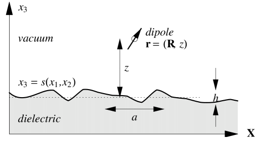
Figure 1: Geometry of the problem. The surface $x_{3}=s(x_{1},x_{2})$ separates the dielectric below (index $n$) from vacuum above. Three different length scales are involved: the dipole’s distance $z$ from the mean surface, the vertical surface corrugation $h$ and the lateral corrugation scale $a$. The transition wavelength $\lambda$ is not shown: typically, $z,\,h,\,a<\lambda$ in near-field microscopy.

These distances are large compared to the dipole’s dimensions, ensuring its purely electromagnetic interactions with the surface. Moreover, it is appropriate to describe the solid by a local dielectric function $\varepsilon(\mathbf{x};\omega)$, allowing the description of the electromagnetic field phenomenologically by Maxwell equations.

The substrate surface is given by the equation $x_{3}=s(x_{1},x_{2})$ where $\mathbf{x}=(x_{1},x_{2},x_{3})$ are cartesian coordinates. The surface corrugation is characterized by two length scales: the typical height $h$ of the vertical corrugation and its lateral scale of variation $a$. In the case of a surface relief grating $h$ would be the grating amplitude and $a$ its period. In the region below the surface, $x_{3}<s(x_{1},x_{2})$, the dielectric function is equal to the squared index of refraction $n^{2}$ that is assumed to be real. The dipole is located in vacuum at the position $\mathbf{r}=(x,y,z)$. We explicitly retain its lateral coordinates $x,y$ since we are interested in the lateral resolution obtained in the variations of the linewidth and lineshift. In order to simplify the formulas, we shall use the notations $\mathbf{X}=(x_{1},x_{2})$ and $\mathbf{R}=(x,y)$ for the lateral coordinates.

2.2 Linewidth and frequency shift

To begin with, let us focus on a system with two energy-levels, a ground state $E_{\mathrm{g}}$ and an excited state $E_{\mathrm{e}}$ connected by an electric dipole transition. We assume that the transition dipole is oriented parallel to the $x_{j}$-axis ($j=1,2,3$, linear polarization) and write $\mathcal{D}_{j}$ for the dipole matrix element. When this atom interacts with the electromagnetic field its energy levels get shifted by amounts $\delta E_{\mathrm{g,e}}(\mathbf{r})$, and the excited state acquires a finite lifetime $1/\Gamma_{j}(\mathbf{r})$ where $\Gamma_{j}(\mathbf{r})$ is the spontaneous emission rate. Both linewidth and level shifts may be calculated in second-order perturbation theory. One obtains the spontaneous emission rate [21]

$$\Gamma_{j}(\mathbf{r})=\frac{\mathcal{D}_{j}^{2}}{\hbar^{2}}\int\limits_{-\infty}^{\infty}\!\mathrm{d}\tau\,\langle\mathrm{vac}|E_{j}^{(+)}(\mathbf{r},t+\tau)E_{j}^{(-)}(\mathbf{r},t)|\mathrm{vac}\rangle\mathrm{e}^{\mathrm{i}\omega_{\mathrm{eg}}\tau}$$ (1)

where $\mathbf{E}^{(\pm)}(\mathbf{r},t)$ are the positive and negative frequency parts of the electric field operator at the atom’s position $\mathbf{r}$, and $\omega_{\mathrm{eg}}=(E_{\mathrm{e}}-E_{\mathrm{g}})/\hbar$ is the atomic transition frequency. At this point one often proceeds to a mode expansion of the electric field operator, and the linewidth (1) connects to squared mode function amplitudes. We take here a different route, following the response theory developed by Agarwal [22], and Wiley and Sipe [23]. More specifically, we invoke the the fluctuation–dissipation–theorem to connect the linewidth $\Gamma_{j}$ to the classical Green function $G_{ij}(\mathbf{x},\mathbf{r};\omega)$. This Green function describes the electric field $\mathbf{E}_{\mathrm{dip}}(\mathbf{x})\mathrm{e}^{-\mathrm{i}\omega t}+\mbox{c.c.}$ (the ‘dipole field’) created by an oscillating point dipole $\mathbf{d}\mathrm{e}^{-\mathrm{i}\omega t}+\mbox{c.c.}$ located at $\mathbf{r}$:

$${E}_{\mathrm{dip},i}(\mathbf{x})=\sum_{j}G_{ij}(\mathbf{x},\mathbf{r};\omega)d_{j}.$$ (2)

The fluctuation–dissipation–theorem allows one to express the linewidth (1) in the following form [22, 23]

$$\Gamma_{j}(\mathbf{r})=\frac{2\mathcal{D}_{j}^{2}}{\hbar}\mathop{\rm Im}\,G_{jj}(\mathbf{r},\mathbf{r};\omega_{\mathrm{eg}}).$$ (3)

In the vicinity of an interface the electric field radiated by the dipole differs from that in free space: it contains, in addition to the well-known dipole field [24], the field reflected from the surface. We write this field in terms of a Green function $G_{ij}^{\mathrm{r}}(\mathbf{x},\mathbf{r};\omega_{0})$. Upon insertion into Eq.(3), we find the environment-induced modification $\delta\Gamma_{j}(\mathbf{r})$ of the linewidth, that now depends on the atom’s position relative to its inhomogeneous environment. We stress that in the present approach, the linewidth is linearly related to the electric field radiated by the dipole, and it is not necessary to compute squared field mode amplitudes which is a more difficult task in a complex geometry.

Let us now turn to the shift of the atomic resonance frequency $\delta\omega_{\mathrm{eg},j}(\mathbf{r})=(\delta E_{\mathrm{e}}(\mathbf{r})-\delta E_{\mathrm{g}}(\mathbf{r}))/\hbar$ in the presence of an interface. By a calculation similar to the one for the linewidth, Fermi’s Golden Rule yields the following result (obtained from Eq.(2.9) of Ref.[23]):

$$\delta\omega_{\mathrm{eg},j}=-\frac{\mathcal{D}_{j}^{2}}{\hbar}\mathop{\rm Re}\,G_{jj}(\mathbf{r},\mathbf{r};\omega_{\mathrm{eg}})+\frac{4\,\mathcal{D}_{j}^{2}}{\hbar}\int\limits_{0}^{\infty}\!\frac{\mathrm{d}\omega}{2\pi}\frac{\mathop{\rm Im}\,G_{jj}(\mathbf{r},\mathbf{r};\omega)}{\omega_{\mathrm{eg}}+\omega}.$$ (4)

The first term has a similar form as Eq.(3) but involves the real part of the Green function.

For an atom with more than two states one has to take into account allowed dipole transitions to other energy levels. Let us focus on the situation depicted in Fig.2

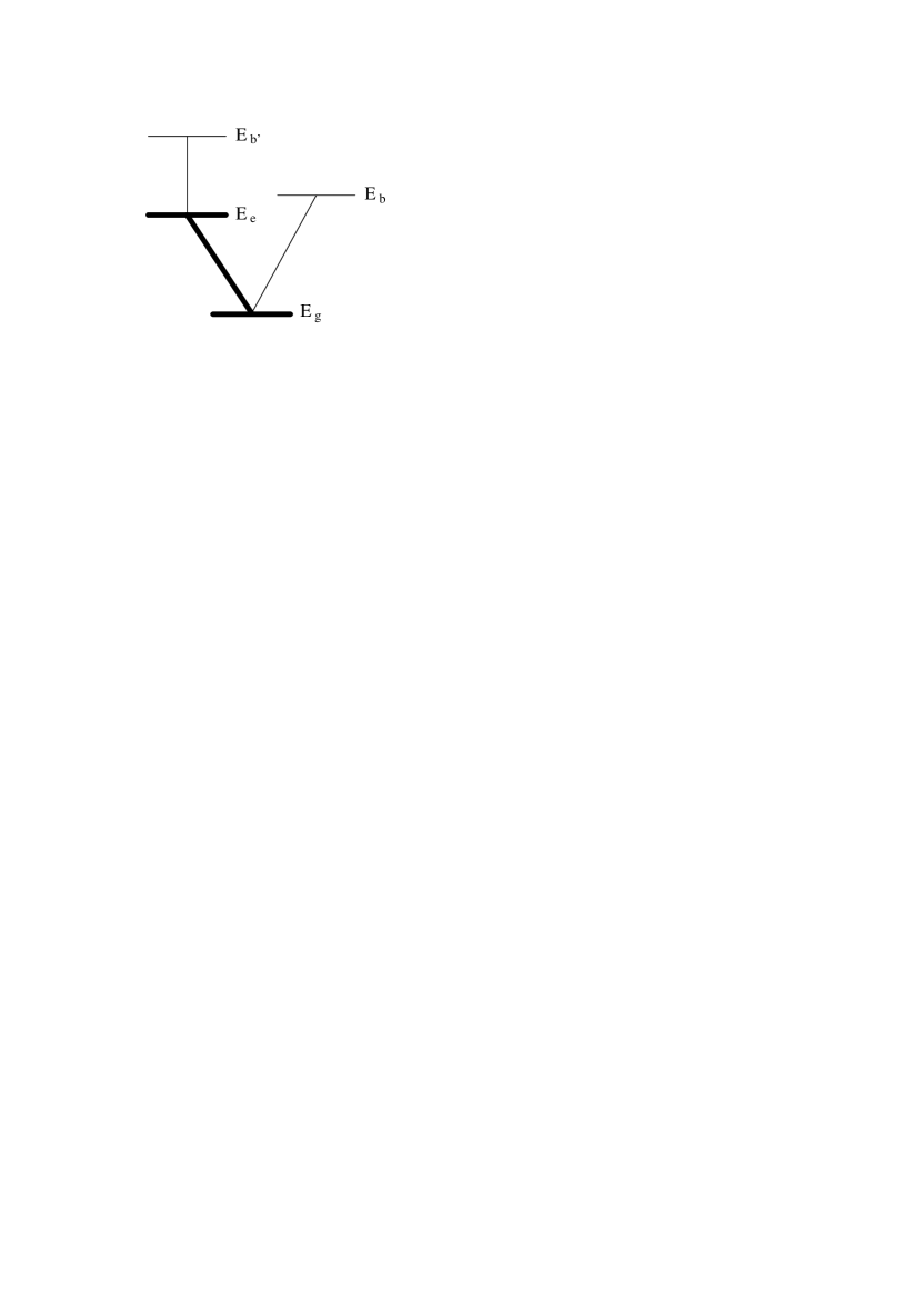
Figure 2: Sketch of a multilevel atom with ground and first excited state.

where the excited level $E_{\mathrm{e}}$ is the first level above the ground state $E_{\mathrm{g}}$. The linewidth $\Gamma_{j}$ is then still given by the two-level expression (1), and the lineshift contains an additional contribution from higher-lying states $E_{\mathrm{b}}$

$$\delta\omega_{\mathrm{eg},j}^{\mathrm{other}}=-\frac{2}{\hbar}\sum_{\mathrm{b},\,E_{\mathrm{b}}>E_{\mathrm{e}}}\int\limits_{0}^{\infty}\!\frac{\mathrm{d}\omega}{2\pi}\mathop{\rm Im}\,G_{jj}(\mathbf{r},\mathbf{r};\omega)\left(\frac{|\langle\mathrm{b}|d_{j}|\mathrm{e}\rangle|^{2}}{\omega_{\mathrm{be}}+\omega}-\frac{|\langle\mathrm{b}|d_{j}|\mathrm{g}\rangle|^{2}}{\omega_{\mathrm{bg}}+\omega}\right).$$ (5)

If the excited state decays to more than one lower-lying level, the decay rate $\Gamma_{j}$ is a sum over several contributions, each one of the form (3).

It is instructive to compare the linewidth (3) and the frequency shift (4) obtained from quantum theory to the corresponding quantities for a classical harmonic oscillator. This model of the Lorentz atom is widely used in the optics community [2, 6, 25, 26], and we can make contact with the work done there. The Lorentz atom is a harmonic oscillator driven by the local electric field, i.e., the external field plus the dipole field (2). Since this field is proportional to the dipole moment itself, it shifts the resonance frequency and leads to a finite damping rate.

For a linearly polarized dipole along the $x_{j}$-axis positioned in an inhomogeneous environment, the shift $\delta\omega_{j}$ and the damping rate $\Gamma_{j}$ are obtained from a straightforward calculation [27]. Normalizing to the free-space linewidth $\Gamma_{\infty}$, one obtains for weak radiation damping (in SI units)

$$\frac{\delta\omega_{j}(\mathbf{r})}{\Gamma_{\infty}}-\frac{\mathrm{i}}{2}\frac{\Gamma_{j}(\mathbf{r})}{\Gamma_{\infty}}=-\frac{3\pi\varepsilon_{0}}{k_{0}^{3}}G_{jj}(\mathbf{r},\mathbf{r};\omega_{0})$$ (6)

where $k_{0}=\omega_{0}/c$ is the vacuum wavenumber. As in the quantum mechanical calculation, the imaginary part of the classical Green function determines the linewidth. The fluorescence rate $\Gamma_{j}$ may thus be computed classically [21], and although we focus in the following on the classical dipole model, our results for the linewidth remain valid for a generic atom. As for the lineshift given by Eq.(6), the classical calculation only yields the first term of the quantum-mechanical results (4, 5), and the nonresonant frequency integrals of the Green function are not accounted for. This implies a limited validity of the classical model for frequency shift calculations. In this paper, however, we are mainly interested in studying the variations in the radiative properties of an atom as a function of its lateral position very close to a structured surface. It is quite common that the atom-surface distances are much smaller than the relevant atomic transition wavelengths. In this regime, the full quantum-mechanical lineshift (4, 5) approximately yields the electrostatic result

$$\delta\omega_{\mathrm{eg},j}\approx-\frac{\langle e|d_{j}^{2}|e\rangle-\langle g|d_{j}^{2}|g\rangle}{\hbar}\mathop{\rm Re}\,G_{jj}(\mathbf{r},\mathbf{r};\omega=0).$$ (7)

Note that this shift is again determined by a classical Green function, in this case at zero frequency. The prefactor is different, however, from the classical dipole and involves the difference in size of the electronic wave function in the ground and excited states (a difference that cancels for a two-level atom [28]). As far as the lateral resolution is concerned, we may therefore treat the case of a classical dipole and use Eq.(6) for simplicity. The exact magnitudes of the line shifts and linewidths for realistic molecules can be then easily calculated considering the above-mentioned discussion.

3 Reflected field calculation

3.1 Outline

Our task is now to compute the Green function above the substrate, i.e., the reflected field created by an oscillating point dipole. The basic equations are the macroscopic Maxwell equations, given the dielectric function $\varepsilon(\mathbf{x};\omega)$ and the external current $\mathbf{j}(\mathbf{x},t)=-\mathrm{i}\omega_{0}\mathbf{d}\delta(\mathbf{x}-\mathbf{r})\mathrm{e}^{-\mathrm{i}\omega_{0}t}+\mbox{c.c.}$, supplemented by the boundary conditions for the field at the surface. We make the following ansatz for the electric field in vacuum above the solid

$$\mathbf{E}(\mathbf{x},t)=\left(\mathbf{E}^{\mathrm{fs}}(\mathbf{x})+\mathbf{E}^{\mathrm{r}}(\mathbf{x})\right)\mathrm{e}^{-\mathrm{i}\omega_{0}t}+\mbox{c.c.}$$ (8)

where $\mathbf{E}^{\mathrm{fs}}(\mathbf{x})$ is the dipole field in free space, and $\mathbf{E}^{\mathrm{r}}(\mathbf{x})$ is its environment-induced modification (the reflected field). The latter is source-free above the surface. The total field (8) is matched at the surface of the solid to a ‘transmitted field’ (source-free inside the solid). This matching determines the reflected and transmitted fields in terms of the free space dipole field.

In general the boundary conditions are complicated, and exact solutions are only known for simple geometries. In order to proceed analytically, we resort to an approximate solution for a ‘slightly corrugated surface’, i.e., a vertical corrugation small compared to the separation of the molecule from the surface. The precise validity of this approximation is discussed in Sec.6. The boundary conditions may then be linearized around the mean value of the surface function and solved to first order in the surface corrugation. We thus end up with three terms for the linewidth

$$\Gamma_{j}(\mathbf{r})=\Gamma_{\infty}+\delta\Gamma_{j}^{0}(z)+\delta\Gamma_{j}^{1}(\mathbf{R},z)$$ (9)

The first term is the vacuum linewidth. The second comes from the reflection at the flat surface (zeroth order field), and the third from the first-order scattering off the surface corrugation. This last term contains information about the lateral surface structure since it depends on the lateral coordinate $\mathbf{R}=(x,y)$. A relation similar to (9) also holds for the frequency shift $\delta\omega_{j}(\mathbf{r})$.

3.2 Approximate solution

In order to find the reflected field to first order, we use the so-called ‘method of small perturbations’ well-known in light scattering from rough surfaces [29, 30, 31]. With this method, one usually computes the reflected field for an incident plane wave. We thus expand the free space dipole field into Fourier components and work out the reflected field for each component. This approach is similar to that of Rahman and Maradudin [32] and of George and co-workers [13, 33].

3.2.1 Fourier expansions

The free space dipole field is well known and may be found from the following formula for the Green function (in SI units) [24, 31]

$$G_{ij}^{\mathrm{fs}}(\mathbf{x},\mathbf{r};\omega)=\left(\frac{\partial^{2}}{\partial x_{i}\,\partial x_{j}}+\delta_{ij}k_{0}^{2}\right)\frac{\exp{\mathrm{i}k_{0}|\mathbf{x}-\mathbf{r}|}}{4\pi\varepsilon_{0}|\mathbf{x}-\mathbf{r}|}$$ (10)

with the wavenumber $k_{0}=\omega/c$. Using the notation $\mathbf{K}=(k_{1},k_{2})$ for the lateral wave vector components and recalling the notations $\mathbf{x}=(\mathbf{X},x_{3})$, $\mathbf{r}=(\mathbf{R},z)$ etc. for the lateral and vertical coordinates, the Weyl expansion reads [31]:

$$\frac{\exp{\mathrm{i}k_{0}|\mathbf{x}-\mathbf{r}|}}{4\pi\varepsilon_{0}|\mathbf{x}-\mathbf{r}|} = \int\!\frac{\mathrm{d}^{2}K}{(2\pi)^{2}}\frac{\mathrm{i}}{2\varepsilon_{0}\,k_{3}}$$

$$\times\exp{\mathrm{i}[\mathbf{K}\cdot(\mathbf{X}-\mathbf{R})+k_{3}|x_{3}-z|]}$$

Here, the vertical wave vector component $k_{3}$ is defined by

$$k_{3}=\sqrt{k_{0}^{2}-\mathbf{K}^{2}}$$ (12)

and the square root is chosen such that $\mathrm{Re}\,k_{3},\,\mathrm{Im}\,k_{3}>0$. It is important to note that the expansion (3.2.1) contains both ‘far field’ and ‘near field’ contributions, corresponding to lateral wave vectors with magnitude ${K}$ smaller and larger than the optical wavenumber $k_{0}$, respectively.

Combining Eqs.(2, 10, 3.2.1), we find the following Fourier expansion for the dipole field in the region $x_{3}<z$ below the dipole:

$$\mathbf{E}^{\mathrm{fs}}(\mathbf{x})=\int\!\frac{\mathrm{d}^{2}K}{(2\pi)^{2}}\mathbf{E}^{\mathrm{fs}}(\mathbf{K})\exp{\mathrm{i}(\mathbf{K}\cdot\mathbf{X}-k_{3}x_{3})}$$ (13)

where the ‘incident wave vector’ is $\mathbf{k}=(\mathbf{K},-k_{3})$ and the dipole field’s Fourier components equal

$$\mathbf{E}^{\mathrm{fs}}(\mathbf{K})=\frac{\mathrm{i}}{2\varepsilon_{0}\,k_{3}}\left[k_{0}^{2}\mathbf{d}-\mathbf{k}(\mathbf{k}\cdot\mathbf{d})\right]\exp{\mathrm{i}(-\mathbf{K}\cdot\mathbf{R}+k_{3}z)}$$ (14)

Since this vector is perpendicular to $\mathbf{k}$, it may be conveniently expanded into two transverse polarization vectors $\mathbf{e}_{\mu}(\mathbf{K})$ labelled by the index $\mu=\mathrm{s},\,\mathrm{p}$:

$$\mathbf{E}^{\mathrm{fs}}(\mathbf{K}) = \frac{\mathrm{i}k_{0}^{2}}{2\varepsilon_{0}\,k_{3}}\sum_{\mu}\mathbf{e}_{\mu}(\mathbf{K})\left(\mathbf{e}_{\mu}(\mathbf{K})\cdot\mathbf{d}\right)$$

$$\times\exp{\mathrm{i}(-\mathbf{K}\cdot\mathbf{R}+k_{3}z)}$$

To solve the boundary conditions, the expansion (13) (and its counterpart (16) for the reflected field) is assumed to be valid down to the surface $x_{3}=s(\mathbf{X})$. This is actually a hypothesis, the ‘Rayleigh hypothesis’, as discussed by Nieto-Vesperinas [31]. Note that the present approach also relies on the assumption that the dipole is located above the maximum surface height, otherwise the absolute value $|s(\mathbf{X})-z|$ in Eq.(3.2.1) must be retained which complicates the calculation.

As used by Agarwal [30] we apply the ‘extinction theorem’ [34] and formulate the boundary conditions as integral equations involving the field immediately above and below the surface. The integrand is evaluated at the surface, and only zeroth and first order terms in the profile function $s(\mathbf{R})$ are taken into account. The reflected field thus contains zeroth and first order contributions that are discussed separately in the following.

3.2.2 Zeroth order: flat surface

The zeroth order result for the reflected field is obtained from the reflection of each Fourier component from a flat surface and involves the corresponding Fresnel coefficient $r_{\mu}(K)$. In the expansion

$$\mathbf{E}^{\mathrm{r,0}}(\mathbf{x})=\int\!\frac{\mathrm{d}^{2}K}{(2\pi)^{2}}\mathbf{E}^{\mathrm{r,0}}(\mathbf{K})\exp{\mathrm{i}(\mathbf{K}\cdot\mathbf{X}+k_{3}x_{3})}$$ (16)

the Fourier coefficients are thus

$$\mathbf{E}^{\mathrm{r,0}}(\mathbf{K}) = \frac{\mathrm{i}k_{0}^{2}}{2\varepsilon_{0}\,k_{3}}\sum_{\mu}\mathbf{e}_{\mu}^{\mathrm{r}}(\mathbf{K})r_{\mu}(K)\left(\mathbf{e}_{\mu}(\mathbf{K})\cdot\mathbf{d}\right)$$

$$\times\exp{\mathrm{i}(-\mathbf{K}\cdot\mathbf{R}+k_{3}z)}$$

where the $\mathbf{e}_{\mu}^{\mathrm{r}}(\mathbf{K})$ are the unit polarization vectors for the specularly reflected waves which are transverse to the wave vector $(\mathbf{K},k_{3})$. From this result we read off the reflected Green function for the flat surface and insert it into the general formula (6), giving

$$\frac{\delta\omega_{j}^{0}(z)}{\Gamma_{\infty}}-\frac{\mathrm{i}}{2}\frac{\delta\Gamma_{j}^{0}(z)}{\Gamma_{\infty}}=-\frac{3\pi\mathrm{i}}{2}\int\!\frac{\mathrm{d}^{2}K}{(2\pi)^{2}}\frac{\exp{(2\mathrm{i}k_{3}z)}}{k_{0}k_{3}}\sum_{\mu}{e}_{\mu,j}^{\mathrm{r}}(\mathbf{K})r_{\mu}(K)\,{e}_{\mu,j}(\mathbf{K}).$$ (18)

As expected, this result only depends on the dipole’s distance $z$, and not on its lateral coordinate $\mathbf{R}$. The integral over the azimuthal angle of the two-dimensional wave vector $\mathbf{K}$ may be done analytically, and one finds the familiar expressions for a dipole oriented perpendicular ($\perp$) or parallel ($\|$) to the surface [2]:

$$\frac{\delta\omega_{\perp}^{0}(z)}{\Gamma_{\infty}}-\frac{\mathrm{i}}{2}\frac{\delta\Gamma_{\perp}^{0}(z)}{\Gamma_{\infty}} = \frac{3\mathrm{i}}{4}\int\limits_{0}^{\infty}\!\mathrm{d}u\,\frac{u^{3}r_{\mathrm{p}}}{\sqrt{1-u^{2}}}\exp{(2\mathrm{i}k_{0}z\sqrt{1-u^{2}})}$$ (19)

$$\frac{\delta\omega_{\|}^{0}(z)}{\Gamma_{\infty}}-\frac{\mathrm{i}}{2}\frac{\delta\Gamma_{\|}^{0}(z)}{\Gamma_{\infty}} = \frac{3\mathrm{i}}{8}\int\limits_{0}^{\infty}\!\mathrm{d}u\,\frac{u}{\sqrt{1-u^{2}}}\left((1-u^{2})r_{\mathrm{p}}-r_{\mathrm{s}}\right)\exp{(2\mathrm{i}k_{0}z\sqrt{1-u^{2}})}$$ (20)

The integration variable is the reduced wave vector $u=K/k_{0}$. Note that the integration range $0\leq u\leq n$ corresponds to field modes that are plane waves in at least one half-space: the linewidth only depends on these modes. For modes with larger wave vectors, $u>n$, the phase factor $\mathrm{e}^{2\mathrm{i}k_{3}z}$ and the reflection coefficients $r_{\mu}$ become real and the integrands in Eqs.(19, 20) become purely imaginary. Hence these modes only appear in the lineshift. This property does not hold any more when absorption in the dielectric is taken into account [26, 27] because the refraction index $n$ and hence the reflection coefficients $r_{\mu}$ are complex for any wave vector.

3.2.3 First order: lateral structure

The first order contribution to the reflected field is Fourier-expanded as in Eq.(16), and from the calculation outlined above, one finds that the Fourier components equal [30, 35, 36]

$$\mathbf{E}^{\mathrm{r,1}}(\mathbf{K}^{\prime})=\mathrm{i}(n^{2}-1)\mathsf{L}(\mathbf{K}^{\prime})\cdot\int\!\frac{\mathrm{d}^{2}K}{(2\pi)^{2}}k_{0}s(\mathbf{K}^{\prime}-\mathbf{K})\,\mathbf{E}^{\mathrm{tr,0}}(\mathbf{K})\exp{\mathrm{i}(-\mathbf{K}\cdot\mathbf{R}+k_{3}z)}.$$ (21)

We use the notation $\mathbf{K}$ for the wave vectors of the zeroth-order field, as in Eq.(3.2.2), while $\mathbf{K}^{\prime}$ denotes the wave vectors of the scattered field. In Eq.(21), $s(\mathbf{K}^{\prime}-\mathbf{K})$ is the Fourier transform of the surface profile, and $\mathbf{E}^{\mathrm{tr,0}}(\mathbf{K})$ is the Fourier component of the field transmitted by the flat surface given by the Fresnel coefficients $t_{\mu}(K)$. Finally, $\mathsf{L}(\mathbf{K})$ is a $3\times 3$-matrix given by [30]

$$L_{ij}(\mathbf{K})=\frac{k_{0}}{k_{3}+k_{3n}}\mathbb{P}_{ij}^{\|}+\frac{n^{2}K^{2}\mathbb{P}_{ij}^{\perp}-K_{i}K_{j}-(n^{2}k_{3}K_{i}\delta_{3j}+k_{3n}K_{j}\delta_{3i})}{k_{0}(n^{2}k_{3}+k_{3n})}$$ (22)

where $\mathbb{P}^{\|,\perp}$ are projectors parallel and perpendicular to the $xy$-plane (the mean surface) and $k_{3n}=\sqrt{n^{2}k_{0}^{2}-K^{2}}$ is the vertical component of the transmitted wave vector. It is understood that the third component of the in-plane vector $\mathbf{K}$ vanishes.

From the first-order reflected field (21) we find the following contribution to the Green function:

$$G_{ij}^{\mathrm{r,1}}(\mathbf{x},\mathbf{r};\omega) = \mathrm{i}(n^{2}-1)\frac{k_{0}^{2}}{2\varepsilon_{0}}\int\!\frac{\mathrm{d}^{2}K^{\prime}}{(2\pi)^{2}}\sum_{k}{L}_{ik}(\mathbf{K}^{\prime})\int\!\frac{\mathrm{d}^{2}K}{(2\pi)^{2}}\frac{\mathrm{i}}{k_{3n}}k_{0}s(\mathbf{K}^{\prime}-\mathbf{K})$$ (23)

$${}\times\sum_{\mu=\mathrm{s,\,p}}{e}_{\mu,k}^{\mathrm{tr}}(\mathbf{K})t_{\mu}(K){e}_{\mu,j}(\mathbf{K})\exp{\mathrm{i}(\mathbf{K}^{\prime}\cdot\mathbf{X}-\mathbf{K}\cdot\mathbf{R}+k_{3}^{\prime}x_{3}+k_{3}z)}$$

where the unit polarization vectors $\mathbf{e}_{\mu}^{\mathrm{tr}}(\mathbf{K})$ describe the field transmitted through the flat surface. Upon insertion in our formula (6), one finds the first-order contribution to the linewidth and the lineshift.

3.3 Transfer function

We observe in Eq.(23) that each wave vector $\mathbf{K}$ of the free-space dipole field is diffracted by the Fourier component $s(\mathbf{K}^{\prime}-\mathbf{K})$ of the surface profile in such a way that the propagation from the dipole down to the surface and back again gives rise to a phase factor $\exp{\mathrm{i}[(\mathbf{K}^{\prime}-\mathbf{K})\cdot\mathbf{R}+(k^{\prime}_{3}+k_{3})z]}$. This leads to a lateral modulation of lineshift and -width at the ‘grating vector’ $\mathbf{Q}=\mathbf{K}^{\prime}-\mathbf{K}$. It is expedient to choose this wave vector as integration variable in (23). One obtains the following form for the first-order contribution to linewidth and -shift:

$$\frac{\delta\omega_{j}^{1}(\mathbf{r})}{\Gamma_{\infty}}-\frac{\mathrm{i}}{2}\frac{\delta\Gamma_{j}^{1}(\mathbf{r})}{\Gamma_{\infty}}=\int\!\frac{\mathrm{d}^{2}Q}{(2\pi)^{2}}k_{0}s(\mathbf{Q})F_{j}(\mathbf{Q};z)\exp{\mathrm{i}(\mathbf{Q}\cdot\mathbf{R})}$$ (24)

where a dimensionless transfer function

$$F_{j}(\mathbf{Q};z) = \frac{3\pi(n^{2}-1)}{2}\int\!\frac{\mathrm{d}^{2}K}{(2\pi)^{2}}\frac{\exp{\mathrm{i}(k_{3}^{\prime}+k_{3})z}}{k_{0}k_{3n}}$$

$$\times\sum_{\mu=\mathrm{s,\,p}}\sum_{k}{L}_{jk}(\mathbf{K}^{\prime}){e}_{\mu,k}^{\mathrm{tr}}(\mathbf{K})t_{\mu}(K)\,{e}_{\mu,j}(\mathbf{K})$$

has been introduced. In this formula, it is understood that $\mathbf{K}^{\prime}=\mathbf{K}+\mathbf{Q}$ and $k_{3}^{\prime}$ is the corresponding vertical wave vector component (eq.(12)). Eq.(24) shows that $F_{j}(\mathbf{Q})$ determines the relative contribution of the profile’s Fourier components $s(\mathbf{Q})$ to the linewidth and -shift. Of particular interest is the width of this “filter” as a function of the grating vector $\mathbf{Q}$ since it determines the lateral resolution of the image.

We show in Fig.3 contour plots of the imaginary part of the integrand in Eq.(3.3) for two different grating vectors $\mathbf{Q}$. It is apparent that the integrand does not have a simple angular dependence in the plane of wave vectors $\mathbf{K}$. This implies that in contrast to the flat surface case Eq.(18), the angular integral cannot be done analytically here, and the transfer function has to be computed numerically.

 

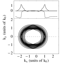
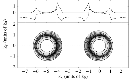
Figure 3: Integrand of the transfer function $F_{3}(\mathbf{Q};z)$ (3.3) as a function of $\mathbf{K}$ in units of the optical wave vector $k_{0}$, for fixed grating vector ${\bf Q}\|{\bf e}_{x}$. Left panel: grating period comparable to wavelength, $\mathbf{Q}=0.8\,k_{0}\,\mathbf{e}_{x}$. Right panel: subwavelength grating period, $\mathbf{Q}=5k_{0}\,\mathbf{e}_{x}$. The contours show the imaginary part, with dark shading indicating large negative values. The inset shows a cut through the dotted horizontal line (solid line: negative imaginary part, dashed line: real part).
The molecule’s distance from the mean grating surface is $k_{0}z=0.3$. Its dipole moment oscillates perpendicular to the mean grating surface (along the $x_{3}$-axis). The substrate index is $n=1.5$. We plot the integrand multiplied by $(2\pi k_{0})^{2}$.

In Fig.3 one or two circular structures appear to dominate the integrand, depending on the magnitude of the grating vector $\mathbf{Q}$. To interpret these features, we come back to the Green function (23) that describes the first-order reflected field. For a given Fourier component $\mathbf{K}$ of the incident dipole field and a given grating vector $\mathbf{Q}=\mathbf{K}^{\prime}-\mathbf{K}$ of the surface profile the scattered field amplitude is equal to the profile’s Fourier amplitude $s(\mathbf{Q})$, multiplied by the product of two factors. The first is an electromagnetic scattering factor represented by the matrix $\mathsf{L}(\mathbf{K}^{\prime})$, the transmission coefficients $t_{\mu}(K)$ and polarization vectors $\mathbf{e}_{\mu}(\mathbf{K})$ for the flat surface. The second factor is the exponential $\exp{\mathrm{i}(k_{3}+k_{3}^{\prime})z}$ describing the vertical propagation of the field from the dipole to the surface and back again. The magnitude of the second factor depends on the character (propagating or evanescent) of the incident and diffracted waves. In particular, the wave vectors $k_{3}$ and $k_{3}^{\prime}$ become imaginary for large $K$, $K^{\prime}$, and the exponential is very small. This limits the relevant range of wave vectors that contribute to the integral.

In the case of the linewidth, the limitation is even more strict. It is determined by the imaginary part of the integrand (cf. Eq.(3.3)) and is given by two circular domains of incident wave vectors $\mathbf{K}$ with $K<nk_{0}$ or $K^{\prime}<nk_{0}$ because it is only in these domains that the exponential $\exp{\mathrm{i}(k_{3}+k_{3}^{\prime})z}$ and the electromagnetic scattering factor become complex. These regions are clearly visible in the right panel of Fig.3. The grating vector $\mathbf{Q}$ is here sufficiently large to separate the two disks. The disks are merged in the left panel because the grating vector is smaller. To summarize, the lateral variation of the linewidth above a corrugated surface is dominated by two different processes: propagating Fourier components of the dipole field are diffracted into evanescent waves and interfere with the dipole field (the right circular disk of Fig.3, centered at $\mathbf{K}=\mathbf{0}$) and conversely, evanescent Fourier components of the dipole field are diffracted into propagating waves (the left disk, centered at $\mathbf{K}=-\mathbf{Q}$).

3.4 Scanning modes

Up to now we have determined the fluorescence spectrum of a molecule at a constant height $z$ above the structured surface. It is also possible to perform these calculations for the more common SNOM scheme of ‘constant-gap’ where the separation of the molecule from the underlying surface profile is kept at a value $d$. In the notation of the present paper one measures the quantity $\Gamma_{j}(\mathbf{R},d+s(\mathbf{R}))$ where $z=d+s(\mathbf{R})$ is the vertical coordinate of the molecule. When calculating this linewidth from Eq.(9) one has to take into account that our theory only describes surface corrugations $s(\mathbf{R})$ small compared to the gap $d$. We thus find a linewidth

$$\Gamma_{j}(\mathbf{R},d+s(\mathbf{R}))=\Gamma_{\infty}+\delta\Gamma_{j}^{0}(d)+s(\mathbf{R})\frac{\partial\delta\Gamma_{j}^{0}(d)}{\partial z}+\delta\Gamma_{j}^{1}(\mathbf{R},d)$$ (26)

The lateral structure is contained in the last two terms, the first of which corresponds to the derivative of the flat-surface linewidth. It turns out that the transfer function for the constant-gap mode can be written in the following form

$$\tilde{F}_{j}(\mathbf{Q};d)=F_{j}(\mathbf{Q};d)-F_{j}(\mathbf{0};d)$$ (27)

where in the second term the constant-height transfer function (3.3) is evaluated at zero wave vector. For simplicity, we focus on the constant-height mode in the rest of this paper .

4 Imaging a grating

We now examine linewidths and -shifts when the dipole is laterally scanned at a constant height above a sinusoidal grating with surface profile $s(\mathbf{R})=s(x)=h\cos Qx$ (grooves parallel to the $y$-axis). This simple geometry reveals the dependence of the radiative properties on the four most important length scales (cf. fig.1): the corrugation height $h$, the corrugation period $a$ (equal to $2\pi/Q$ for a grating), the molecule’s distance $z$ from the average surface and the transition wavelength $\lambda=2\pi/k_{0}$. Finally, one also has to take into account the dipole’s orientation. Translational symmetry implies that linewidth and -shift are independent of $y$, but they are sinusoidal as a function of the lateral position $x$ since they depend linearly on the surface profile (cf. Eq.(24) and Fig.4). All the relevant physics is thus encoded in their modulation amplitude [37]. Since this amplitude is simply proportional to the grating height $h$, this length scale is already dealt with.

In Fig.4 the grating has subwavelength corrugation amplitude ($0.016\,\lambda$) and period ($0.1\,\lambda$), the substrate is a dielectric with refractive index $n=1.5$ (glass) and negligible absorption, while the dipole is polarized perpendicular to the grating surface ($z$-polarization). We observe that at an average distance from the grating of $0.032\,\lambda$, the linewidth modulation amounts to 20 % of the natural linewidth. A much larger modulation is observed in the lineshift which amounts up to several natural linewidths. We would like to stress this feature because frequency shifts have not been considered very much in the optics community, perhaps because they are more difficult to measure. Our calculations show that in near-field optics, the lineshift is much more sensitive (on an absolute frequency scale) to the surface corrugation than the linewidth. This relatively large effect is related to the large frequency shift close to a flat surface, as discussed in subsection 4.2.

  

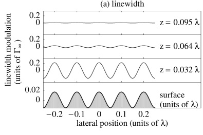
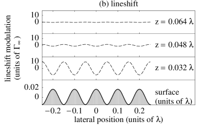
Figure 4: The modulations in the linewidth $\delta\Gamma^{1}(x,z)$ (a) and lineshift $\delta\omega^{1}(x,z)$ (b) of a dipole with vertical polarization at a fixed height above a sinusoidal grating. The grating is made in a glass substrate ($n=1.5$) and has period $a=\lambda/10$ and amplitude $h=0.1\,\lambda/(2\pi)\approx 0.016\,\lambda$. Note the difference in scale between linewidth and -shift.

We discuss the dependence of linewidth and lineshift on the distance from the grating and its period in the next two sections.

4.1 The linewidth

In fig.5(a) we show the amplitude of the linewidth modulation above a grating with subwavelength period, as a function of the distance $z$. One observes that the three dipole orientations show different behavior, and that the linewidth modulation decreases rapidly with increasing distance from the grating. This decrease is quite well fitted with an exponential law $\mathrm{e}^{-Qz}$, as shown in the inset. Such a law is to be expected since as discussed at the end of section 3.3, the linewidth is dominated by diffraction processes where the incoming wave has a small parallel wave vector (see fig.3, right panel). The diffracted wave then has a parallel component with wave vector $\mathbf{K}^{\prime}\approx\mathbf{Q}$ whose amplitude decays exponentially $\propto\mathrm{e}^{-Qz}$ if the grating vector $Q$ is much larger than $k_{0}$. This is the phenomenon which allows one to exploit the modifications of the lifetime to image nanometric structures in the near field. Fig.5(a) also shows deviations from a pure exponential decay of the linewidth, we come back to these in eq.(29).

  

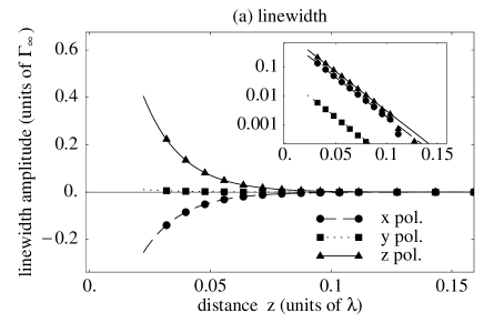
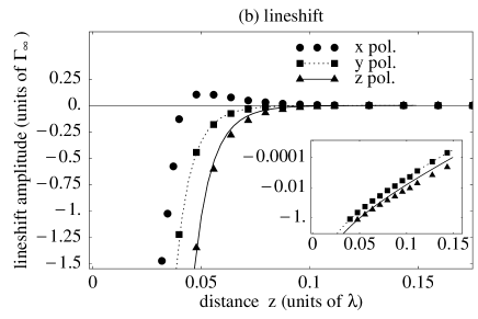
Figure 5: The amplitude of the linewidth (a) and lineshift (b) modulations vs. distance from a dielectric sinusoidal grating (index $n=1.5$) with period $a=\lambda/10$ and amplitude $h=0.1\,\lambda/(2\pi)\approx 0.016\,\lambda$. The three linear polarizations are shown. The insets give the same data on a logarithmic scale (the absolute value is taken). In (a), the lines are fits to simple exponentials $\mathrm{e}^{-Qz}$, the amplitude being the only free parameter. In (b), the lines are fits to the model function $K_{2}(Qz)/z^{2}$ introduced in eq.(33). For clearness, the $x$-polarization is omitted from the inset. See text for more details.

In Fig.6(a) we plot the amplitude of the linewidth modulation as a function of the average distance $z$ for a large grating period.

  

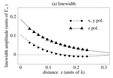
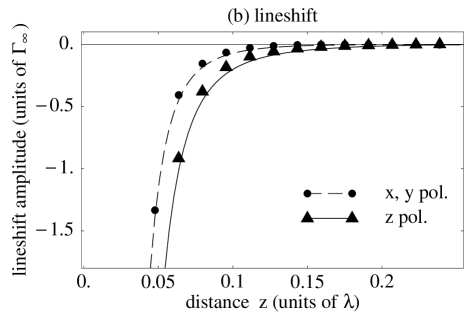
Figure 6: The amplitude of the linewidth modulation (a) and lineshift modulation (b) vs. distance $z$ from a dielectric sinusoidal grating (index $n=1.5$) with period $a=5\,\lambda$ and amplitude $h=0.1\,\lambda/(2\pi)\approx 0.016\,\lambda$. Thin lines: simple model (28) involving the derivative of the flat surface result (see text for details).

One observes that the modulation amplitude decreases more slowly than in fig.5(a) and even shows oscillations for distances of the order of the wavelength. In the extreme case of grating period much larger than the wavelength this behavior of the linewidth may be understood in a simple manner. In this case one may write the linewidth modulation in the form

$$a\gg\lambda:\quad\delta\Gamma(x,z)\approx\delta\Gamma^{0}(z-s(x))\approx\delta\Gamma^{0}(z)-s(x)\frac{\partial\delta\Gamma^{0}}{\partial z}$$ (28)

The linewidth modulation amplitude turns out to be proportional to the derivative of the flat surface result. In Fig.6(a), the result of this model is indicated by the thin lines which coincide quite well with the full calculation (symbols) although the grating period is taken to be only $5\,\lambda$. We note, however, that in this simple model the two lateral polarizations $x$ and $y$ are always degenerate since they both derive from the linewidth $\delta\Gamma_{\|}^{0}(z)$ of a dipole polarized parallel to a flat surface.

Fig.7(a) shows the modulations of the linewidth as a function of the grating vector $Q$ for a fixed height $z$. We observe that grating periods larger than $\lambda$ ($Q\ll k_{0}$) yield a result similar to that of a flat surface, $x$- and $y$-polarization being degenerate. As the period decreases below the wavelength, this degeneracy is lifted, and we observe an overall increase in the linewidth modulation with some steep features for $Q\leq 2nk_{0}$.

  

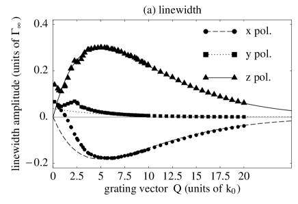
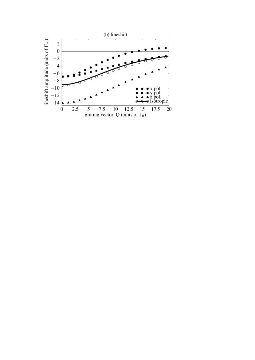
Figure 7: Amplitude of the linewidth modulation (a) and lineshift modulation (b) vs. grating vector for a dipole at a distance of $z=0.2\,\lambda/(2\pi)\approx 0.032\,\lambda$ from the mean surface. The three linear polarizations are shown. (a) The lines give the linewidth modulation obtained from the asymptotic formula (29). (b) The open dots close to the thick line give the lineshift for an isotropic dipole, and the thick line itself shows the simple model of Eq.(33). The electrostatic value of the coefficient $c_{3}$ is $(\Gamma_{\infty}/8k_{0}^{3})(n^{2}-1)/(n^{2}+1)$.

For still smaller grating periods the linewidth modulation decreases again in an approximately exponential manner.

It is possible to give an asymptotic expression for the transfer function (3.3) covering the regime of subwavelength corrugations which is particularly interesting for applications in optical near-field microscopy. This asymptotic expansion is motivated by Fig.3 (right panel) where we have seen that the integrand of the transfer function is dominated by two circular regions of wave vectors. In the limit of $\mathbf{Q}$ large compared to $k_{0}$ these regions are well separated and have approximately circular symmetry. In both cases the angular integrations may be performed analytically, and one arrives at formulae very similar to those for a flat surface (19, 20). For the three linear polarizations one obtains:

$$Q\gg k_{0}:\quad\mathop{\rm Im}\,F_{j}(\mathbf{Q};z)\approx\frac{3}{4}\frac{n^{2}-1}{n^{2}+1}\mathrm{e}^{-Qz}\left(\frac{Q}{k_{0}}\right)^{\alpha_{j}}\mathop{\rm Im}\,f_{j}(z)$$ (29)

Here, the exponent is $\alpha_{j}=1$ for the $j=x,z$ polarizations, and $\alpha_{y}=0$ for $j=y$. If the distance $z$ is much smaller than the wavelength, the (complex) dimensionless functions $f_{j}(z)$ ($j=x,y,z$) that correct the pure exponential decay in eq.(29) are given by [38]

$$f_{x}(z) = 4\int\limits_{0}^{nk_{0}}\frac{K\,\mathrm{d}K}{k_{0}^{2}}\mathrm{e}^{\mathrm{i}k_{3}z}\left(\frac{k_{0}}{k_{3}+k_{3n}}-\frac{K^{2}}{2k_{0}(n^{2}k_{3}+k_{3n})}\right)$$ (30)

$$f_{y}(z) = -\left(n^{2}+\mathrm{i}\right)\int\limits_{0}^{nk_{0}}\frac{K^{3}\,\mathrm{d}K}{k_{0}^{4}}\frac{k_{3}\,\mathrm{e}^{\mathrm{i}k_{3}z}}{n^{2}k_{3}+k_{3n}}$$ (31)

$$f_{z}(z) = -4\mathrm{i}\int\limits_{0}^{nk_{0}}\frac{K^{3}\,\mathrm{d}K}{k_{0}^{4}}\frac{n^{2}k_{0}\,\mathrm{e}^{\mathrm{i}k_{3}z}}{n^{2}k_{3}+k_{3n}}$$ (32)

It can be seen from Fig.7(a) that these asymptotic formulae give an excellent representation for the modulation of the linewidth above subwavelength gratings with periods $a\leq\lambda/5$. We may therefore use eqs.(29–32) to estimate the lateral resolution $\delta R$ for this type of near-field microscopy: the exponential cutoff of high spatial frequencies in Eq.(29) yields $\delta R\simeq z$, the distance from the surface. Note also that the $y$-polarization gives both a smaller signal and a slightly worse resolution compared to the other two polarizations, which is due to the missing of the factor $Q/k_{0}$ in Eq.(29). This is physically plausible because the electric field is then continuous across the interface, leading to less scattering from the surface corrugation.

4.2 The lineshift

Apart from its larger modulation amplitude, the lineshift above a sinusoidal grating shows a behavior not very different from that of the linewidth. In fig.5(b) the grating period is subwavelength, and one observes again a rapid decrease of the modulation amplitude with increasing distance. Vector diffraction is relevant and leads to different results for the three polarizations, the $x$-polarization in particular showing a sign change (dots). At distances larger than $1/Q$, the lineshift shows an exponential decrease similar to the linewidth, as shown by the solid and dotted lines. These lines are fits to the model function $K_{2}(Qz)/z^{2}$ introduced in eq.(33) below.

The case of a grating period larger than the wavelength is shown in fig.6(b). The $x$- and $y$-polarizations show identical lineshifts as above a flat surface. The distance dependence is well described by the simple model based on eq.(28), involving the derivative of the flat-surface result. In particular, the lineshift shows a $1/z^{4}$ power law if the dipole’s distance is smaller than about $\lambda/(2\pi)$, as expected from electrostatics.

Finally, fig.7(b) displays the amplitude of the lineshift modulation if the grating period is varied. The $x,y$-polarizations show smooth crossovers from large to small periods, and the modulation amplitude globally decreases for very small periods. This latter feature can be understood from a simple electrostatic calculation, as we discuss now.

We model the substrate as a continuous distribution of dipoles (with density $\rho_{\mathrm{dip}}$) with which the molecule interacts via a (scalar) $c_{6}/r^{6}$ law. The total frequency shift is obtained by integrating over the half-space filled with these dipoles. For a flat substrate one obtains the familiar power law $\delta\omega^{0}(z)=-c_{3}/z^{3}$ with $c_{3}=\pi\rho_{\mathrm{dip}}c_{6}/6$. If the substrate is corrugated, the surface region gives an additional contribution to the frequency shift. To first order in the surface profile, one obtains:

$$z\ll\frac{\lambda}{2\pi}:\quad\delta\omega^{1}(\mathbf{Q};z)\approx-s(\mathbf{Q})\frac{3c_{3}}{2}\frac{Q^{2}}{z^{2}}K_{2}(Qz)$$ (33)

where $\delta\omega^{1}(\mathbf{Q};z)$ is a Fourier transform with respect to the lateral coordinates $\mathbf{R}$ and $K_{2}(Qz)$ is the modified Bessel function of the second kind. As we show in fig.7(b), this simple model (thick solid line) describes quite well the frequency shift for an unpolarized dipole (averaged over the three linear polarizations, shown by the open circles). For large periods the shift becomes independent of $Q$ and tends to $-3c_{3}/z^{4}$, the derivative of the flat-surface shift (this follows from the properties of the Bessel $K$-function) while for small periods we find an exponential suppression similar to eq.(29):

$$Qz\gg 1:\quad\delta\omega^{1}(\mathbf{Q};z)\approx-s(\mathbf{Q})\frac{3c_{3}\sqrt{\pi}}{2\sqrt{2}}\frac{Q^{3/2}\mathrm{e}^{-Qz}}{z^{5/2}}$$ (34)

In this model we may thus explain the suppression of high spatial frequencies in the lineshift variations by the fact that the frequency shift samples a patch of the surface whose radius is of order $z$, thus washing out structures at lateral scales smaller than $a\leq z$. As a consequence, we expect for lineshift images a lateral resolution of the order of $z$.

We finally note that similar to the linewidth (29), the lineshift (34) above a subwavelength grating does not show a pure exponential decay with increasing distance $z$ (see also inset of fig.5(b)).

5 Imaging an arbitrary substrate

As pointed out above, our theory is linear in the surface corrugation and hence able to describe both sinusoidal and arbitrary profiles. An example of a generic (two-dimensional) surface is shown in Fig.8.

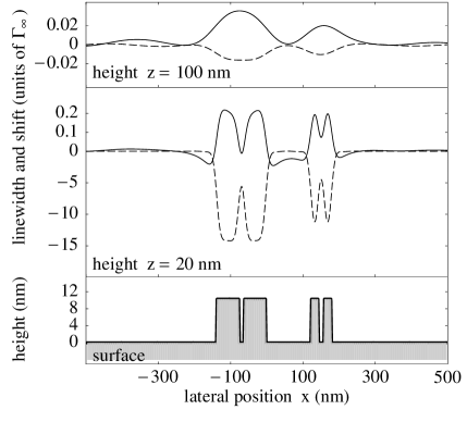
Figure 8: Linewidth and lineshift ‘images’ of surface topography. The surface profile is shown in the bottom panel (thick line, in nm). The mid and top panels show linewidth (thin solid line) and lineshift (dashed line) at two different constant heights above the mean surface, in units of the free-space linewidth $\Gamma_{\infty}$. Only the laterally modulated parts $\delta\Gamma^{1}(x,z)$ and $\delta\omega^{1}(x,z)$ are shown. Note the difference in scale for the lineshift at height $z=20$ nm. Dielectric substrate with index $n=1.5$. Transition wavelength $\lambda=628$ nm. Vertical polarization.

One observes a low lateral resolution and quite a weak signal at an average height $z=100~{}\mathrm{nm}\approx\lambda/2\pi$ (top panel) with the linewidth and -shift having comparable magnitudes. The situation changes dramatically at closer distances ($z=20~{}\mathrm{nm}\approx 0.2\,\lambda/2\pi$, middle panel) where subwavelength structures are well resolved. Note that the linewidth gives a slightly poorer ‘image quality’ than the lineshift. This is due to the fact that the spectral response of the lineshift behaves more smoothly as a function of wave vector than that of the linewidth (compare figs.7(a) and (b)). In other words, some spatial frequencies are enhanced in the linewidth image, leading to a distortion of the observed structures.

One advantage of optical near-field microscopy over other scanning probe techniques is its ability to yield information beyond the sample topography, namely about its optical contrast. In fact, often samples with large topographic features are undesirable in SNOM because they lead to the coupling of the optical and topographic information [39, 40]. It is important to point out that our theory also applies to substrates with purely optical contrast and no topography. For this we use the result of Carminati and Greffet that in near-field optics variations of the dielectric constant may be described by an ‘equivalent surface profile’ $s_{\mathrm{eq}}(\mathbf{X})$ [41]. This quantity corresponds to the vertical integral of the optical contrast:

$$s_{\mathrm{eq}}(\mathbf{X})=\int\limits_{-\infty}^{\infty}\!\mathrm{d}x_{3}\,\left[\varepsilon(\mathbf{X},x_{3})-\varepsilon_{\mathrm{flat}}(x_{3})\right]$$ (35)

where $\varepsilon_{\mathrm{flat}}(x_{3})$ is the dielectric function of a flat reference substrate. In fig.9 we show an example of such a substrate where objects with larger indices are buried in a flat substrate.

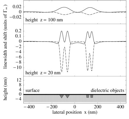
Figure 9: Fluorescence image of a sample with optical contrast. In the dark-shaded region, four objects with a larger index $n=2.5$ are buried in the flat substrate with $n=1.5$. Thin solid line: linewidth, dashed line: lineshift. The other parameters are identical to fig.8.

6 Limitations of the approximation

The first-order calculation is crucially dependent on the linearized boundary conditions at the ‘slightly corrugated surface’. More precisely, this means that for all relevant Fourier components the following expansion must remain sufficiently accurate:

$$\exp{\ \mathrm{i}[(k_{3}+k_{3}^{\prime})s(\mathbf{X})]}\approx 1+\mathrm{i}(k_{3}+k_{3}^{\prime})s(\mathbf{X})$$ (36)

where $k_{3}$ and $k_{3}^{\prime}$ are the wave vectors of the incident dipole field and the diffracted field, respectively. For far-field calculations, $k_{3}$ and $k_{3}^{\prime}$ are real and limited to the optical wave vector $k_{0}$. Therefore, we obtain the condition $|s(\mathbf{X})|\leq h\ll\lambda/2\pi$, where $h$ characterizes the surface corrugation. For calculations in the near field one has to include imaginary values of $k_{3}$ and $k_{3}^{\prime}$. The relevant wave vectors, however, are limited in size because the finite distance $z$ leads to an exponential damping; this is also apparent in Eq.(3.3). We hence find the condition $h\ll z$. Finally, for a grating with a period $a$ well below $\lambda$ all diffraction orders are evanescent, and the diffracted wave vectors are of the order of $k_{3}^{\prime}\simeq Q=2\pi/a$. In order to perform the linearization (36) in this regime, we have to impose the condition $h\ll a$. In summary, our method is valid in the regime

$$h\ll\min\{a,\,\lambda,\,z\}$$ (37)

Note that no restriction is made regarding the relative magnitude of the three length scales on the right-hand-side. For a sample with optical contrast it is shown in Ref.[41] that the perturbation method is also subject to condition (37), but now for the equivalent surface profile. In particular, this is the case if the index inhomogeneities are confined to a narrow region around the interface, below which the sample is homogeneous.

7 Concluding remarks

The theory presented here may be generalized to take absorption of the substrate into account. In the classical picture this is simply done by using a complex index of refraction. In the quantum mechanical picture several schemes have been proposed [42, 43, 44, 45] to quantize the electromagnetic field in the presence of absorbing dielectrics, involving different models for the dielectric medium. Using the theory of Scheel, Knöll, and Welsch [45], it is easy to check that the fluctuation-dissipation theorem still holds. The identification of the field correlation function in Eq.(1) with the imaginary part of the classical Green function in Eq.(3) hence carries over to the absorbing substrate. From the viewpoint of quantum optics this substantiates the use of the classical Lorentz oscillator to compute the fluorescence lifetime of real molecules in arbitrary environments.

We now would like to remark on a few physical effects which take place beyond the regime (37) and therefore, are not taken into account by our current treatment:

(i) If the grating corrugation is comparable to the wavelength $h\sim\lambda$, one expects many diffraction orders to be populated. In this regime the calculation of the reflected field has to be refined using a full grating theory. At large distances from such a ‘deep grating’ the physics should be quite similar to standard far-field grating diffraction. At smaller distances the molecule samples non-propagating diffraction orders, and evanescent components of the incidence dipole field could lead to qualitative changes of the linewidth. If the grating’s ‘depth’ exceeds several wavelengths, one may expect the formation of a partial photonic band gap, modifying the near field. Since for a complete band gap only evanescent light modes are present, molecular fluorescence would be a very interesting probe to study the electromagnetic field in such structures. In a future paper we intend to consider a grating with a square profile for which an exact diffraction theory is available [46, 47, 48, 49].

(ii) If the molecule is put into the selvedge region of the grating, i.e. $z\leq h$, it is nearly completely surrounded by the substrate. One then expects that only the local environment plays a role, the molecule being unable to sense the periodicity of the grating. Numerical calculations have been done [17, 18, 50] which show steep variations of the lifetime and a strong polarization dependence. We plan to study the square grating model alluded to above to get an analytical insight into this situation.

In conclusion, we have calculated the modification of the fluorescence spectrum of a molecule that is scanned above a slightly corrugated surface. We have shown that the molecule’s linewidth and lineshift are influenced by both surface topography and optical contrast. The linewidth acquires variations that amount up to 20 %, while the lineshift varies over as much as several natural linewidths. Furthermore, for an arbitrary surface profile the lineshift shows a slightly better fidelity to the sample structure. We have also presented simple models and formulae that allow us to obtain an intuitive understanding of the our results for corrugations and distances both below and above the molecular transition wavelength. Perhaps the most important outcome of this paper is that the lateral resolution in the ‘fluorescence images’ we have obtained is of the order of the molecule-surface distance. One would then expect to reach a molecular resolution in a novel form of scanning optical microscopy if the probe molecule could be brought nearly in contact with the sample. Recent experimental progress in the field of single molecule detection, spectroscopy and manipulation give a tantalizing hope for the realization of this goal in the near future.

References

- [1] P. W. Milonni, The Quantum Vacuum (Academic Press Inc., San Diego, 1994).
- [2] R. R. Chance, A. Prock, and R. Silbey, in Advances in Chemical Physics XXXVII, edited by I. Prigogine and S. A. Rice (Wiley & Sons, New York, 1978).
- [3] E. A. Hinds and V. Sandoghdar, Phys. Rev. A 43, 398 (1991).
- [4] H. B. Casimir and D. Polder, Phys. Rev. 73, 360 (1948).
- [5] K. H. Drexhage, in Progress in Optics XII, edited by E. Wolf (North-Holland, Amsterdam, 1974), pp. 163–232.
- [6] For a recent review, see: W. L. Barnes, J. mod. Optics 45, 661 (1998).
- [7] D. J. Heinzen and M. S. Feld, Phys. Rev. Lett. 59, 2623 (1987).
- [8] V. Sandoghdar, C. I. Sukenik, E. A. Hinds, and S. Haroche, Phys. Rev. Lett. 68, 3432 (1992).
- [9] M. Oria, M. Chevrollier, D. Bloch, M. Fichet, and M. Ducloy, Europhys. Lett. 14, 527 (1991).
- [10] W. Knoll, M. R. Philpott, J. D. Swalen, and A. Girlando, J. Chem. Phys. 75, 4795 (1981).
- [11] P. K. Aravind and H. Metiu, Chem. Phys. Lett. 74, 301 (1980).
- [12] P. K. Aravind, E. Hood, and H. Metiu, Surf. Sci. 109, 95 (1981).
- [13] P. T. Leung, Z. C. Wu, D. A. Jelski, and T. F. George, Phys. Rev. B 36, 1475 (1987).
- [14] F. Balzer, V. G. Bordo, and H.-G. Rubahn, Opt. Lett. 22, 1262 (1997).
- [15] W. P. Ambrose, P. M. Goodwin, J. C. Martin, and R. A. Keller, Science 265, 364 (1994).
- [16] R. Kopelman and W. Tan, Science 262, 1382 (1993).
- [17] C. Girard, O. J. F. Martin, and A. Dereux, Phys. Rev. Lett. 75, 3098 (1995).
- [18] A. Rahmani, P. C. Chaumet, F. de Fornel, and C. Girard, Phys. Rev. A 56, 3245 (1997).
- [19] Single Molecule Optical Detection, Imaging and Spectroscopy, edited by T. Basché, W. E. Moerner, M. Orrit, and U. P. Wild (Wiley-VCH, Weinheim, 1997).
- [20] J. Michaelis, C. Hettich, B. Eiermann, J. Mlynek, and V. Sandoghdar, (1998), in preparation.
- [21] W. Heitler, The quantum theory of radiation, 3rd ed. (Oxford University Press, Oxford, 1954).
- [22] G. S. Agarwal, Phys. Rev. A 11, 230 (1975).
- [23] J. M. Wylie and J. E. Sipe, Phys. Rev. A 30, 1185 (1984).
- [24] J. D. Jackson, Classical Electrodynamics, 2nd ed. (Wiley & Sons, New York, 1975), Chap. 7.
- [25] H. Metiu, Progr. Surf. Science 17, 153 (1984).
- [26] G. W. Ford and W. H. Weber, Phys. Rep. 113, 195 (1984).
- [27] S. Haroche, in Fundamental Systems in Quantum Optics (Les Houches, Session LIII), edited by J. Dalibard, J.-M. Raimond, and J. Zinn-Justin (North-Holland, Amsterdam, 1992), pp. 767–940.
- [28] G. Barton, J. Phys. B: Atom. Molec. Phys. 7, 2134 (1974).
- [29] A. A. Maradudin and D. L. Mills, Phys. Rev. B 11, 1392 (1975).
- [30] G. S. Agarwal, Phys. Rev. B 15, 2371 (1977).
- [31] M. Nieto-Vesperinas, Scattering and Diffraction in Physical Optics (Wiley & Sons, New York, 1991).
- [32] T. S. Rahman and A. A. Maradudin, Phys. Rev. B 21, 504 (1980).
- [33] P. T. Leung, T. F. George, and Y. C. Lee, J. Chem. Phys. 86, 7227 (1987).
- [34] M. Born and E. Wolf, Principles of Optics (Pergamon Press, London, 1959).
- [35] J.-J. Greffet, Phys. Rev. B 37, 6436 (1988).
- [36] D. V. Labeke and D. Barchiesi, J. Opt. Soc. Am. A 10, 2193 (1993).
- [37] We have observed that for more complex polarizations, the modulations of linewidth and -shift are ‘phase-shifted’ with respect to the grating profile. This is formally related to the fact that the Green tensor (23) has nonzero off-diagonal elements.
- [38] For distances not small compared to the wavelength, the integrands in eqs. (30–32) acquire an additional -dependence (not shown for brevity). The first corrections are of relative order .
- [39] B. Hecht, H. Bielefeldt, Y. Inouye, D. W. Pohl, and L. Novotny, J. Appl. Phys. 81, 2492 (1997).
- [40] V. Sandoghdar, S. Wegscheider, G. Krausch, and J. Mlynek, J. Appl. Phys. 81, 2499 (1997).
- [41] R. Carminati and J.-J. Greffet, J. Opt. Soc. Am. A 12, 2716 (1995).
- [42] B. Huttner, J. J. Baumberg, and S. M. Barnett, Europhys. Lett. 16, 177 (1991).
- [43] M. S. Yeung and T. K. Gustafson, Phys. Rev. A 54, 5227 (1996).
- [44] H. T. Dung, L. Knöll, and D.-G. Welsch, Phys. Rev. A 57, 3931 (1998).
- [45] S. Scheel, L. Knöll, and D.-G. Welsch, Phys. Rev. A 58, 700 (1998).
- [46] A. Wirgin and R. Deleuil, J. Opt. Soc. Am. 59, 1348 (1969).
- [47] D. Maystre and R. Petit, Opt. Commun. 5, 90 (1972).
- [48] I. C. Botten, M. S. Craig, R. C. McPhedran, J. L. Adams, and J. R. Andrewartha, Optica Acta 28, 413 (1981).
- [49] P. Sheng, R. S. Stepleman, and P. N. Sanda, Phys. Rev. B 26, 2907 (1982).
- [50] L. Novotny, Appl. Phys. Lett. 69, 3806 (1996).