Structure of T –  and S – Matrices in Unphysical Sheets and Resonances in Three – Body Systems

Abstract

Algorithm, based on explicit representations for the analytic continuation of Faddeev components of the three-body T-matrix in unphysical energy sheets, is employed to study mechanism of disappearance and formation of the Efimov levels of the helium ⁴He trimer.

1 Introduction

Explicit representations for the Faddeev components of the three-body T-matrix continued analytically into unphysical sheets of the energy Riemann surface have been formulated and proved recently in Ref. [1]. According to the representations, the T-matrix in unphysical sheets is explicitly expressed in terms of its components only taken in the physical sheet. Analogous explicit representations were also found for the analytic continuation of the three-body scattering matrices. These representations disclose the structure of kernels of the T- and S-matrices after continuation and give new capacities for analytical and numerical studies of the three-body resonances. In particular the representations imply that the resonance poles of the S-matrix as well as T-matrix in an unphysical sheet correspond merely to the zeros of the suitably truncated three-body scattering matrix taken in the physical sheet. Therefore, one can search for resonances in a certain unphysical sheet staying always, nevertheless, in the physical sheet and only calculating the position of zeros of the appropriate truncation of the total three-body scattering matrix. This statement holds true not only for the case of the conventional smooth quickly decreasing interactions but also for the case of the singular interactions described by different variants of the Boundary Condition Model, in particular for the inter–particle interactions of a hard-core nature like in most molecular systems.

As a concrete application of the method, we present here the results of our numerical study of the simplest truncation of the scattering matrix in the ⁴He three-atomic system, namely of the $(2+1\to 2+1)$ S-matrix component corresponding to the scattering of a ⁴He atom off a ⁴He dimer. The point is that there is already a series of works [2]–[4] (also see Refs. [5]–[7]) showing that the excited state of the ⁴He trimer is initiated by the Efimov effect  [8]. In these works, various versions of the ⁴He–⁴He potential were employed. However, the basic result of Refs. [2]–[4] on the excited state of the helium trimer is the same: this state disappears after the interatomic potential is multiplied by the increasing factor $\lambda$ when it approaches the value about 1.2. It is just such a nonstandard behavior of the excited-state energy as the coupling between helium atoms becomes more and more strengthening, points to the Efimov nature of the trimer excited state. The present work is aimed at elucidating the fate of the trimer excited state upon its disappearance in the physical sheet when $\lambda>1$ and at studying the mechanism of arising of new excited states when $\lambda<1$. As the interatomic He – He potential, we use the potential HFD-B [9]. We have established that for such He – He - interactions the trimer excited-state energy merges with the two-body threshold $\epsilon_{d}$ at $\lambda\approx 1.18$ and with further decreasing $\lambda$ it transforms into a virtual level of the first order (a simple real pole of the analytic continuation of the $(2+1\to 2+1)$ scattering matrix component) lying in the unphysical energy sheet adjoining the physical sheet along the spectral interval between $\epsilon_{d}$ and the three–body threshold. We trace the position of this level for $\lambda$ increasing up to 1.5. Besides, we have found that the excited (Efimov) levels for $\lambda<1$ also originate from virtual levels of the first order that are formed in pairs. Before a pair of virtual levels appears, there occurs a fusion of a pair of conjugate resonances of the first order (simple complex poles of the analytic continuation of the scattering matrix in the unphysical sheet) resulting in the virtual level of the second order.

2 Representations for three-body T –  and S – matrices
in unphysical energy sheets

The method used for calculation of resonances in the present work, is based on the explicit representations [1] for analytic continuation of the T- and scattering matrices in unphysical sheets which hold true at least for a part of the three-body Riemann surface. To describe this part we introduce the auxiliary vector-function ${\mathfrak{f}}(z)=({\mathfrak{f}}_{0}(z),{\mathfrak{f}}_{1,1}(z),...,{\mathfrak{f}}_{1,n_{1}}(z),$ ${\mathfrak{f}}_{2,1}(z),...,{\mathfrak{f}}_{2,n_{2}}(z),$ ${\mathfrak{f}}_{3,1}(z),...,{\mathfrak{f}}_{3,n_{3}}(z))$    with $\enspace{\mathfrak{f}}_{0}(z)$ $=$ $\ln{z}$ and ${\mathfrak{f}}_{\alpha,j}(z)$ $=$ $(z-\lambda_{\alpha,j})^{1/2}.$ Here, by $z$ we understand the total three-body energy in the c. m. system and by $\lambda_{\alpha,j}$, the respective binding energies of the two-body subsystems $\alpha,$ $\alpha=1,2,3,$ $j=1,2,...,n_{\alpha}$, $n_{\alpha}<\infty$. The sheets $\Pi_{l}$ of the Riemann surface of the vector-function ${\mathfrak{f}}(z)$ are numerated by the multi-index $l=(l_{0},l_{1,1},...,l_{1,n_{1}},l_{2,1},...,l_{2,n_{2}},l_{3,1},...,l_{3,n_{3}}),$ where $l_{\alpha,j}=0$ if the sheet $\Pi_{l}$ corresponds to the main (arithmetic) branch of the square root $(z-\lambda_{\alpha})^{1/2}.$ Otherwise, $l_{\alpha,j}=1$ is assumed. Value of $l_{0}$ coincides with the number of the branch of the function $\ln{z}$, $\ln z=\ln|z|+\,{\rm i}\,2\pi l_{0}+{\rm i}\phi$ where $\phi=\mathop{\rm arg}z$. For the physical sheet identified by $l_{0}=l_{\alpha,j}=0$, $\alpha=1,2,3,\enspace j=1,2,...,n_{\alpha}$, we use the notation $\Pi_{0}$.

Surely, the structure of the total three-body Riemann surface is essentially more complicated than that of the auxiliary function ${\mathfrak{f}}$. For instance, the sheets $\Pi_{l}$ with $l_{0}=\pm 1$ have additional branching points corresponding to resonances of the two-body subsystems. The part of the total three-body Riemann surface where the representations of Ref. [1] are valid, consists of the sheets $\Pi_{l}$ of the Riemann surface of the function ${\mathfrak{f}}$ identified by $l_{0}=0$ (such unphysical sheets are called two-body sheets) and two three-body sheets identified by $l_{0}=\pm 1$ and $l_{\alpha,j}=1,$ $\alpha=1,2,3,$ $j=1,2,...,n_{\alpha}.$

In what follows by $k_{\alpha},p_{\alpha}$ ($k_{\alpha},p_{\alpha}\in{\mathbb{R}}^{3}$ or $k_{\alpha},p_{\alpha}\in{\mathbb{C}}^{3}$) we understand the standard reduced relative momenta of the three-body system while $P=\{k_{\alpha},p_{\alpha}\}$ ($P\in{\mathbb{R}}^{6}$ or $P\in{\mathbb{C}}^{6}$) stands for the total relative momentum.

The representations [1] for the analytic continuation of the matrix ${\bf M}(z)=\left\{M_{\alpha\beta}(z)\right\},\alpha,\beta=1,2,3,$ of the Faddeev components $M_{\alpha\beta}(z)$ (see [10]) of the three-body $T$-operator, into the sheet $\Pi_{l}$ read as follows:

$${\bf M}(z)\biggr{|}_{\Pi_{l}}={\bf M}(z)-{\bf B}^{\dagger}(z)A(z)L{\rm S}_{l}^{-1}(z)\widetilde{L}{\bf B}(z).$$ (1)

Here, the factor $A(z)$ is the diagonal matrix, $A(z)=\mathop{\rm diag}\{A_{0}(z),$ $A_{1,1}(z),$ $\ldots,$ $A_{1,n_{3}}(z)\}$ with $A_{0}(z)=-\pi{\rm i}z^{2}$ and $A_{\alpha,j}=-\pi{\rm i}\sqrt{z-\lambda_{\alpha,j}},$ $j=1,2,...,n_{\alpha}$. Notations $L$ and $\widetilde{L}$ stand for the diagonal number matrices combined of the indices of the sheet $\Pi_{l}$: $L=\mathop{\rm diag}\{l_{0},l_{1,1},...,l_{3,n_{3}}\}$ and $\widetilde{L}=\mathop{\rm diag}\{|l_{0}|,l_{1,1},...,l_{3,n_{3}}\}.$ By ${\rm S}_{l}(z)$ we understand a truncation of the three-body scattering matrix ${\rm S}(z)$ defined in $\widehat{\cal G}=L_{2}(S^{5})\mathop{\oplus}\limits_{\alpha=1}^{3}\mathop{\oplus}\limits_{j=1}^{n_{\alpha}}L_{2}(S^{2})$ by the equation

$${\rm S}_{l}(z)=\widehat{I}+\widetilde{L}\bigl{[}{\rm S}(z)-\widehat{I}\bigr{]}L$$

where $\widehat{I}$ is the identity operator in $\widehat{\cal G}$. Also, we use the notations

$${\bf B}(z)=\left(\begin{array}[]{l}{\rm J}_{0}\Omega{\bf M}\\ {\rm J}_{1}\mathchoice{{\hbox{\boldmath$\displaystyle\Psi$\unboldmath}}}{{\hbox{\boldmath$\textstyle\Psi$\unboldmath}}}{{\hbox{\boldmath$\scriptstyle\Psi$\unboldmath}}}{{\hbox{\boldmath$\scriptscriptstyle\Psi$\unboldmath}}}^{*}[\Upsilon{\bf M}+{\bf v}]\end{array}\right)\mbox{\,\,and\,\,}{\bf B}^{\dagger}(z)=\left({\bf M}(z)\Omega^{\dagger}{\rm J}_{0}^{\dagger},[{\bf v}+{\bf M}\Upsilon]\mathchoice{{\hbox{\boldmath$\displaystyle\Psi$\unboldmath}}}{{\hbox{\boldmath$\textstyle\Psi$\unboldmath}}}{{\hbox{\boldmath$\scriptstyle\Psi$\unboldmath}}}{{\hbox{\boldmath$\scriptscriptstyle\Psi$\unboldmath}}}{\rm J}^{\dagger}_{1}\right).$$

Here, ${\bf v}=\mathop{\rm diag}\{v_{1},v_{2},v_{3}\}$ with $v_{\alpha}$, the pair potentials, $\alpha=1,2,3$. At the same time, $\Omega=(1,\,\,1,\,\,1),$ $\Upsilon=\{\Upsilon_{\alpha\beta}\}$ with $\Upsilon_{\alpha\beta}=1-\delta_{\alpha\beta}$, $\alpha,\beta=1,2,3,$ and $\mathchoice{{\hbox{\boldmath$\displaystyle\Psi$\unboldmath}}}{{\hbox{\boldmath$\textstyle\Psi$\unboldmath}}}{{\hbox{\boldmath$\scriptstyle\Psi$\unboldmath}}}{{\hbox{\boldmath$\scriptscriptstyle\Psi$\unboldmath}}}=\mathop{\rm diag}\{\mathchoice{{\hbox{\boldmath$\displaystyle\Psi$\unboldmath}}}{{\hbox{\boldmath$\textstyle\Psi$\unboldmath}}}{{\hbox{\boldmath$\scriptstyle\Psi$\unboldmath}}}{{\hbox{\boldmath$\scriptscriptstyle\Psi$\unboldmath}}}_{1},\mathchoice{{\hbox{\boldmath$\displaystyle\Psi$\unboldmath}}}{{\hbox{\boldmath$\textstyle\Psi$\unboldmath}}}{{\hbox{\boldmath$\scriptstyle\Psi$\unboldmath}}}{{\hbox{\boldmath$\scriptscriptstyle\Psi$\unboldmath}}}_{2},\mathchoice{{\hbox{\boldmath$\displaystyle\Psi$\unboldmath}}}{{\hbox{\boldmath$\textstyle\Psi$\unboldmath}}}{{\hbox{\boldmath$\scriptstyle\Psi$\unboldmath}}}{{\hbox{\boldmath$\scriptscriptstyle\Psi$\unboldmath}}}_{3}\}$ where $\mathchoice{{\hbox{\boldmath$\displaystyle\Psi$\unboldmath}}}{{\hbox{\boldmath$\textstyle\Psi$\unboldmath}}}{{\hbox{\boldmath$\scriptstyle\Psi$\unboldmath}}}{{\hbox{\boldmath$\scriptscriptstyle\Psi$\unboldmath}}}_{\alpha},$ $\alpha=1,2,3,$ are operators acting on $f=(f_{1},f_{2},...,f_{n_{\alpha}})\in\mathop{\oplus}\limits_{j=1}^{n_{\alpha}}L_{2}({\mathbb{R}}^{3})$ as $(\mathchoice{{\hbox{\boldmath$\displaystyle\Psi$\unboldmath}}}{{\hbox{\boldmath$\textstyle\Psi$\unboldmath}}}{{\hbox{\boldmath$\scriptstyle\Psi$\unboldmath}}}{{\hbox{\boldmath$\scriptscriptstyle\Psi$\unboldmath}}}_{\alpha}f)(P)=\sum\limits_{j=1}^{n_{\alpha}}\psi_{\alpha,j}(k_{\alpha})f_{j}(p_{\alpha})$ where, in turn, $\psi_{\alpha,j}$ is the bound-state wave function of the pair subsystem $\alpha$ corresponding to the binding energy $\lambda_{\alpha,j}$. By $\mathchoice{{\hbox{\boldmath$\displaystyle\Psi$\unboldmath}}}{{\hbox{\boldmath$\textstyle\Psi$\unboldmath}}}{{\hbox{\boldmath$\scriptstyle\Psi$\unboldmath}}}{{\hbox{\boldmath$\scriptscriptstyle\Psi$\unboldmath}}}^{*}$ we denote operator adjoint to $\textstyle\Psi$. Notation ${\rm J}_{0}(z)$ is used for the operator restricting a function on the energy-shell $|P|^{2}=z$. The diagonal matrix-valued function ${\rm J}_{1}(z)=\mathop{\rm diag}\{{\rm J}_{1,1}(z),...,{\rm J}_{3,n_{3}}(z)\}$ consists of the operators ${\rm J}_{\alpha,j}(z)$ of restriction on the energy surfaces $|p_{\alpha}|^{2}=z-\lambda_{\alpha,j}.$ The operators $\Omega^{\dagger}$, ${\rm J}_{0}^{\dagger}(z)$ and ${\rm J}^{\dagger}_{1}(z)$ represent the “transposed” matrices $\Omega$, ${\rm J}_{0}(z)$ and ${\rm J}_{1}(z)$, respectively. Operators ${\rm J}_{0}^{\dagger}(z)$ and ${\rm J}^{\dagger}_{1}(z)$ act in the expression for ${\bf B}^{\dagger}$ (as if) to the left.

With some stipulations (see [1]) the representations for the scattering matrix read

$${\rm S}(z)\biggr{|}_{\Pi_{l}}={\cal E}(l)\left\{\widehat{I}+{\rm S}_{l}^{-1}(z)[{\rm S}(z)-\widehat{I}]e(l)\right\}{\cal E}(l).$$ (2)

Here, ${\cal E}=\mathop{\rm diag}\{{\cal E}_{0},{\cal E}_{1,1},...,{\cal E}_{3,n_{3}}\}$ where ${\cal E}_{0}$ is the identity operator in $L_{2}(S^{5})$ if $l_{0}=0$ and inversion, $({\cal E}_{0}f)(\widehat{P})=f(-\widehat{P}),$ if $l_{0}=\pm 1$. Analogously, ${\cal E}_{\alpha,j}$ is the identity operator in $L_{2}(S^{2})$ for $l_{\alpha,j}=0$ and inversion for $l_{\alpha,j}=1.$ Notation $e(l)$ is used for the diagonal number matrix $e(l)=\mathop{\rm diag}\{e_{0},e_{1,1},...,e_{3,n_{3}}\}$ with nontrivial elements $e_{\alpha,j}=1$ if $l_{\alpha,j}=0$ and $e_{\alpha,j}=-1$ if $l_{\alpha,j}=1;$ for all the cases $e_{0}=1$.

It follows from the representations (1) and (2) that the resonances (the nontrivial poles of ${\bf M}(z)\biggr{|}_{\Pi_{l}}$ and ${\rm S}(z)\biggr{|}_{\Pi_{l}}$) situated in the unphysical sheet $\Pi_{l}$ are those points $z=z_{\rm res}$ in the physical sheet where the matrix ${\rm S}_{l}(z)$ has zero as eigenvalue. Therefore, calculation of resonances in the unphysical sheet $\Pi_{l}$ is reduced to a search for zeros of the respective truncation ${\rm S}_{l}(z)$ of the scattering matrix ${\rm S}(z)$ in the physical sheet.

3 Method for search of resonances in a three–body system
on the basis of the Faddeev differential equations

In this work we discuss the example of the three-atomic ⁴He system at the total angular momentum $L=0$. We consider the case where the interatomic interactions include a hard core component and, outside the hard core domain, are described by conventional smooth potentials. In this case, the angular partial analysis reduces the initial Faddeev equation for three identical bosons to a system of coupled two-dimensional integro-differential equations (see Ref. [4] and references therein)

$$\left[-\frac{\partial^{2}}{\partial x^{2}}-\frac{\partial^{2}}{\partial y^{2}}+l(l+1)\left(\frac{1}{x^{2}}+\frac{1}{y^{2}}\right)-E\right]F_{l}(x,y)$$ (6)

$$=\left\{\begin{array}[]{cl}-V(x)\mathchar 265\relax_{l}(x,y),&x>c\\ 0,&x<c\,.\end{array}\right.$$

Here, $x,y$ stand for the standard Jacobi variables and $c$, for the core range. At $L=0$ the partial angular momentum $l$ corresponds both to the dimer subsystem and a complementary atom. For the $S$-state three-boson system $l$ is even, $l=0,2,4,\ldots\,.$ In our work, the energy $z$ can get both real and complex values. The He–He potential $V(x)$ acting outside the core domain is assumed to be central. The partial wave function $\mathchar 265\relax_{l}(x,y)$ is related to the Faddeev components $F_{l}(x,y)$ by $\mathchar 265\relax_{l}(x,y)=F_{l}(x,y)+\sum_{l^{\prime}}\int_{-1}^{+1}d\eta\,h_{ll^{\prime}}(x,y,\eta)\,F_{l^{\prime}}(x^{\prime},y^{\prime})$ where $x^{\prime}=(\frac{1}{4}\,x^{2}+\frac{3}{4}\,y^{2}-\frac{\sqrt{3}}{2}\,xy\eta)^{1/2}\,,y^{\prime}=(\frac{3}{4}\,x^{2}+\frac{1}{4}\,y^{2}+\frac{\sqrt{3}}{2}\,xy\eta)^{1/2}\,$ and $1\leq{\eta}\leq 1$. The explicit form of the function $h_{ll^{\prime}}$ can be found in Refs. [10, 11]. The functions $F_{l}(x,y)$ satisfy the boundary conditions

$$F_{l}(x,y)\left.\right|_{x=0}=F_{l}(x,y)\left.\right|_{y=0}=0\,,\qquad\mathchar 265\relax_{l}(c,y)=0\,$$ (7)

Note that the last of these conditions is a specific condition corresponding to the hard-core model (see Ref. [4]).

Here we only deal with a finite number of equations (6), assuming that $l\leq l_{\rm max}$ where $l_{\rm max}$ is a certain fixed even number. The condition $0\leq l\leq l_{\rm max}$ is equivalent to the supposition that the potential $V(x)$ only acts in the two-body states with $l=0,2,\ldots,l_{\rm max}$. The spectrum of the Schrödinger operator for a system of three identical bosons with such a potential is denoted by $\sigma_{3B}$. We assume that the potential $V(x)$ falls off exponentially and, thus, $|V(x)|\leq C\exp(-\mu x)$ with some positive $C$ and $\mu$. For the sake of simplicity we even assume sometimes that $V(x)$ is finite, i. e., $V(x)=0$ for $x>r_{0}$, $r_{0}>0$. Looking ahead, we note that, in fact, in our numerical computations of the ⁴He₃ system at complex energies we make a “cutoff” of the interatomic He – He - potential at a sufficiently large $r_{0}$. The asymptotic conditions as $\rho\rightarrow\infty$ and/or $y\rightarrow\infty$ for the partial Faddeev components of the $(2+1\rightarrow 2+1\,;\,1+1+1)$ scattering wave functions for $z=E+{\rm i}0$, $E>0$, read (see, e. g., Ref. [10])

$$F_{l}(x,y;z) = \delta_{l0}\psi_{d}(x)\left\{\sin(\sqrt{z-\epsilon_{d}}\,y)+\exp({\rm i}\sqrt{z-\epsilon_{d}}\,y)\left[{\rm a}_{0}(z)+o\left(1\right)\right]\right\}$$ (8)

$$+\displaystyle\frac{\exp({\rm i}\sqrt{z}\rho)}{\sqrt{\rho}}\left[A_{l}(z,\theta)+o\left(1\right)\right]\,.$$

We assume that the ⁴He dimer has an only bound state with an energy $\epsilon_{d}$, $\epsilon_{d}<0$, and wave function $\psi_{d}(x)$, $\psi_{d}(x)=0$ for $0\leq x\leq c$. The notations $\rho$, $\rho=\sqrt{x^{2}+y^{2}}$ , and $\theta$, $\theta=\mathop{\rm arctan}(y/x)$, are used for the hyperradius and hyperangle. The coefficient ${\rm a}_{0}(z)$, $z=E+{\rm i}0$, for $E>\epsilon_{d}$ is the elastic scattering amplitude. The functions $A_{l}(E+{\rm i}0,\theta)$ provide us, at $E>0$, the corresponding partial Faddeev breakup amplitudes. For real $z=E+{\rm i}0$, $E>\epsilon_{d}$, the $(2+1{\rightarrow}2+1)$ component of the $s$-wave partial scattering matrix for a system of three helium atoms is given by the expression

$${\rm S}_{0}(z)=1+2{\rm i}{\rm a}_{0}(z)\,.$$

Our goal is to study the analytic continuation of the function ${\rm S}_{0}(z)$ into the physical sheet. As it follows from the results of Refs. [1], the function ${\rm S}_{0}(z)$ is just that truncation of the total scattering matrix whose roots in the physical sheet of the energy $z$ plane correspond to the location of resonances situated in the unphysical sheet adjoining the physical one along the spectral interval $(\epsilon_{d},0)$.

There are the following three important domains in the the physical sheet.

1^∘. The domain $\mathchar 261\relax^{(\mathchar 265\relax)}$ where the Faddeev components $F_{l}(x,y;z)$ (and, hence, the wave functions $\mathchar 265\relax_{l}(x,y;z)$) can be analytically continued in $z$ so that the differences $\mathchar 264\relax_{l}(x,y;z)=F_{l}(x,y;z)-\delta_{l0}\psi_{d}(x)\sin(\sqrt{z-\epsilon_{d}}\,y)$ at $z\in\mathchar 261\relax^{(\mathchar 265\relax)}\setminus\sigma_{3B}$ are square integrable. This domain is described by the inequality

$$\mathop{\rm Im}\sqrt{z-\epsilon_{d}}<{\rm min}\left\{\frac{\sqrt{3}}{2}\mu,\,\sqrt{3}\sqrt{|\epsilon_{d}|}\right\}\,.$$

2^∘. The domain $\mathchar 261\relax^{(A)}$ where both the elastic scattering amplitude ${\rm a}_{0}(z)$ and the Faddeev breakup amplitudes $A_{l}(z,\theta)$ can be analytically continued in $z$, $z\not\in\sigma_{3B}$, and where the continued functions $F_{l}(x,y;z)$ still obey the asymptotic formulas (8). This domain is described by the inequalities

$$\mathop{\rm Im}\sqrt{z}+\frac{1}{2}\mathop{\rm Im}\sqrt{z-\epsilon_{d}}<\frac{\sqrt{3}}{2}\sqrt{|\epsilon_{d}|},\quad\mathop{\rm Im}\sqrt{z}+\mathop{\rm Im}\sqrt{z-\epsilon_{d}}<\frac{\sqrt{3}}{2}\mu\,.$$

3^∘. And finally, we distinguish the domain $\mathchar 261\relax^{(S)}$, most interesting for us, where the analytic continuation in $z$, $z\not\in\sigma_{3B}$, can be only done for the amplitude ${\rm a}_{0}(z)$ (and consequently, for the scattering matrix ${\rm S}_{0}(z)$); the analytic continuabilty of the amplitudes $A_{l}(z,\theta)$ in the whole domain $\mathchar 261\relax^{(S)}$ is not required. The set $\mathchar 261\relax^{(S)}$ is a geometric locus of points obeying the inequality

$$\mathop{\rm Im}\sqrt{z-\epsilon_{d}}<\mathop{\rm min}\left\{\frac{1}{\,\sqrt{3}\,}\,\sqrt{|\epsilon_{d}|},\,\frac{\,\sqrt{3}\,}{2}\mu\right\}\,.$$

Since the spherical wave $\exp({\rm i}\sqrt{z}\,\rho)/\sqrt{\rho}$ in Eq. (8) is a function rapidly decreasing in all the directions, the use of the asymptotic condition (8) is justified even if $z\in\mathchar 261\relax^{(S)}\setminus\mathchar 261\relax^{(A)}$. Outside of the domain $\mathchar 261\relax^{(S)}$ the numerical construction of ${\rm S}_{0}(z)$ by solving the Faddeev differential equations is, in general, impossible.

4 Numerical results

In the present work we search for the resonances of the ⁴He trimer including the virtual levels as roots of ${\rm S}_{0}(z)$ and for the bound-state energies as positions of poles of ${\rm S}_{0}(z)$. All the results presented below are obtained for the case $l_{\rm max}=0$. In all our calculations, $\hbar^{2}/m=12.12$ K Ų. As the interatomic He – He - interaction we employed the HFD-B potential constructed by R. A. Aziz and co-workers [9].

The value of the core range $c$ is chosen to be so small that its further decrease does not appreciably influence the dimer binding energy $\epsilon_{d}$ and the trimer ground-state energy $E_{t}^{(0)}$. Unlike the paper [4], where $c$ was taken to be equal 0.7 Å, now we take $c=1.3$ Å. We have found that such a value of $c$ provides at least six reliable figures of $\epsilon_{d}$ and three figures of $E_{t}^{(0)}$.

Since the statements of Sect. 3 are valid, generally speaking, only for the potentials decreasing not slower than exponentially, we cut off the potential HFD-B setting $V(x)=0$ for $x>r_{0}$. We have established that this cutoff for $r_{0}\gtrsim 95$ Å provides the same values of $\epsilon_{d}$ ($\epsilon_{d}=-1.68541$ mK), $E_{t}^{(0)}$ ($E_{t}^{(0)}=-0.096$ K) and scattering phases which were obtained in earlier calculations [4] performed with the potential HFD-B. Also, we have found that the trimer excited-state energy $E_{t}^{(1)}=-2.46$ mK. Comparison of these results with results of other researchers can be found in Ref. [4]. In all the calculations of the present work we take $r_{0}=100$ Å. Note that if the formulas from Sect. 3 describing the holomorphy domains $\mathchar 261\relax^{(\mathchar 265\relax)}$, $\mathchar 261\relax^{(A)}$ and $\mathchar 261\relax^{(S)}$ are used for finite potentials, one should set in them $\mu=+\infty$.

A detailed description of the numerical method we use is presented in Ref. [4]. When solving the boundary-value problem (6–8) we carry out its finite-difference approximation in polar coordinates $\rho$ and $\theta$. In this work, we used the grids of dimension $N_{\theta}=N_{\rho}=$ 600 — 1000. In essential, we chose the values of the cutoff hyperradius $\rho_{\rm max}=\rho_{N_{\rho}}$ from the scaling considerations (see [4]). We solve the resultant block-three-diagonal algebraic system on the basis of the matrix sweep method. This allows us to dispense with writing the system matrix on the hard drive and to carry out all the operations related to its inversion immediately in RAM. Besides, the matrix sweep method reduces almost by one order the computer time required for computations on the grids of the same dimensions as in [4].

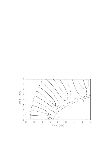
Figure 1: Root locus curves of the real and imaginary parts of the scattering matrix ${\rm S}_{0}(z)$. The solid lines correspond to $\mathop{\rm Re}{\rm S}_{0}(z)=0$, while the tiny dashed lines, to $\mathop{\rm Im}{\rm S}_{0}(z)=0$. The numbers 1, 2 and 3 denote the boundaries of the domains $\mathchar 261\relax^{(\mathchar 265\relax)}$, $\mathchar 261\relax^{(S)}$ and $\mathchar 261\relax^{(A)}$, respectively. Complex roots of the function ${\rm S}_{0}(z)$ are represented by the intersection points of the curves $\mathop{\rm Re}{\rm S}_{0}(z)=0$ and $\mathop{\rm Im}{\rm S}_{0}(z)=0$ and are located at $(-2.34+{\rm i}\,0.96)$ mK, $(-0.59+{\rm i}\,2.67)$ mK, $(2.51+{\rm i}\,4.34)$ mK and $(6.92+{\rm i}\,6.10)$ mK.

Because of the symmetry relationship $\overline{{\rm S}_{0}(z)}={{\rm S}_{0}(\overline{z})}$ we performed all the calculations for ${\rm S}_{0}(z)$ only at $\mathop{\rm Im}z\geq 0$. First, we calculated the root lines of the functions $\mathop{\rm Re}{\rm S}_{0}(z)$ and $\mathop{\rm Im}{\rm S}_{0}(z)$. For the case of the grid parameters $N_{\theta}=N_{\rho}=600$ and $\rho_{\rm max}=600$ Å these lines are depicted in Fig. 1. Both resonances (roots of ${\rm S}_{0}(z)$) and bound-state energies (poles of ${\rm S}_{0}(z)$) of the ⁴He trimer are associated with the intersection points of the curves $\mathop{\rm Re}{\rm S}_{0}(z)=0$ and $\mathop{\rm Im}{\rm S}_{0}(z)=0$. In Fig. 1, along with the root lines we also plot the boundaries of the domains $\mathchar 261\relax^{(S)}$, $\mathchar 261\relax^{(A)}$ and $\mathchar 261\relax^{(\mathchar 265\relax)}$. One can observe that the “good” domain $\mathchar 261\relax^{(S)}$ includes none of the points of intersection of the root lines $\mathop{\rm Re}{\rm S}_{0}(z)=0$ and $\mathop{\rm Im}{\rm S}_{0}(z)=0$. The caption for Fig. 1 points out positions of four “resonances”, the roots of ${\rm S}_{0}(z)$, found immediately beyond the boundary of the domain $\mathchar 261\relax^{(S)}$. It is remarkable that the “true” (i. e., getting inside $\mathchar 261\relax^{(S)}$) virtual levels and then the energies of the excited (Efimov) states appear just due to these (quasi)resonances when the potential $V(x)$ is weakened.

Following [2]–[4], instead of the initial potential $V(x)=V_{\rm HFD-B}(x)$, we, further, consider the potentials $V(x)=\lambda\cdot V_{\rm HFD-B}(x).$ To establish the mechanism of formation of new excited states in the ⁴He trimer, we have first calculate the scattering matrix ${\rm S}_{0}(z)$ for $\lambda<1$.

Table 4.1: Dependence of the dimer binding energy $\epsilon_{d}$ and the differences $\epsilon_{d}-E_{t}^{(1)}$, $\epsilon_{d}-E_{t}^{(2)}$, $\epsilon_{d}-E_{t}^{(2)*}$ and $\epsilon_{d}-E_{t}^{(2)**}$ (all in mK) between this energy and the trimer exited-state energies $E_{t}^{(1)}$, $E_{t}^{(2)}$ and the virtual-state energies $E_{t}^{(2)*}$, $E_{t}^{(2)**}$ on the factor $\lambda$.

$\lambda$	$\epsilon_{d}$	$\epsilon_{d}-E_{t}^{(1)}$	$\epsilon_{d}-E_{t}^{(2)*}$	$\epsilon_{d}-E_{t}^{(2)**}$	$\epsilon_{d}-E_{t}^{(2)}$
0.995	$-1.160$	0.710	–	–	–
0.990	$-0.732$	0.622	–	–	–
0.9875	$-0.555$	0.573	0.473	0.222	–
0.985	$-0.402$	0.518	0.4925	0.097	–
0.980	$-0.170$	0.39616	0.39562	0.009435	–
0.975	$-0.036$	0.2593674545	0.2593674502	–	0.00156

In Table 4.1 for some values of $\lambda$ from the interval between 0.995 and 0.975, we present the positions of roots and poles of ${\rm S}_{0}(z)$, we have obtained at real $z<\epsilon_{d}(\lambda)$. We have found that for a value of $\lambda$ slightly smaller than $0.9885$, the (quasi)resonance closest to the real axis (see Fig. 1) gets on it and transforms into a virtual level (the root of ${\rm S}_{0}(z)$) of the second order corresponding to the energy value where the graph of ${\rm S}_{0}(z)$, $z\in{\mathbb{R}}$, $z<\epsilon_{d}$, is tangent to the axis $z$. This virtual level is preceded by the (quasi)resonances $z=(-1.04+{\rm i}\,0.11)$ mK for $\lambda=0.989$ and $z=(-0.99+{\rm i}\,0.04)$ mK for $\lambda=0.9885$. With a subsequent decrease of $\lambda$ the virtual level of the second order splits into a pair of the first order virtual levels $E_{t}^{(2)*}$ and $E_{t}^{(2)**}$, $E_{t}^{(2)*}<E_{t}^{(2)**}$ which move in opposite directions. A characteristic behavior of the scattering matrix ${\rm S}_{0}(z)$ when the resonances transform into virtual levels is shown in Fig. 2. The virtual level $E_{t}^{(2)**}$ moves towards the threshold $\epsilon_{d}$ and “collides” with it at $\lambda<0.98$. For $\lambda=0.975$ the function ${\rm S}_{0}(z)$ has no longer the root corresponding to $E_{t}^{(2)**}$. Instead of the root, it acquires a new pole corresponding to the second excited state of the trimer with the energy $E_{t}^{(2)}$. We expect that the subsequent Efimov levels originate from the virtual levels just according to the same scheme as the level $E_{t}^{(2)}$ does.

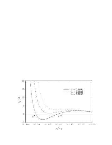
Figure 2: Graphs of the function ${\rm S}_{0}(z)$ at real $z\leq\epsilon_{d}$ for three values of $\lambda<1$ . The notations used: $E^{*}=E_{t}^{(2)*}/|\epsilon_{d}|$, $E^{**}=E_{t}^{(2)**}/|\epsilon_{d}|$.

The other purpose of the present investigation is to determine the mechanism of disappearance of the excited state of the helium trimer when the two-body interactions become stronger owing to the increasing $\lambda>1$. It turned out that this disappearance proceeds just according to the scheme of the formation of new excited states; only the order of occurring events is inverse. The results of our computations of the energy $E_{t}^{(1)}$ when $\lambda$ changes from 1.05 to 1.17 are given in Table 4.2.

Table 4.2: Dependence of the dimer energy $\epsilon_{d}$, the difference $\epsilon_{d}-E_{t}^{(1)}$ between $\epsilon_{d}$ and the trimer exited-state energy $E_{t}^{(1)}$ and the difference $\epsilon_{d}-E_{t}^{(1)*}$ between $\epsilon_{d}$ and the trimer virtual-state energy $E_{t}^{(1)*}$ (all in mK) on the factor $\lambda$.

$\lambda$	$\epsilon_{d}$	$\epsilon_{d}-E_{t}^{(1)}$	$\lambda$	$\epsilon_{d}$	$\epsilon_{d}-E_{t}^{(1)*}$
1.05	$-12.244$	0.873	1.18	$-82.927$	0.001
1.10	$-32.222$	0.450	1.20	$-99.068$	0.057
1.15	$-61.280$	0.078	1.25	$-145.240$	0.588
1.16	$-68.150$	0.028	1.35	$-261.393$	3.602
1.17	$-75.367$	0.006	1.50	$-490.479$	12.276

In the interval between $\lambda=1.17$ and $\lambda=1.18$ there occurs a “jump” of the level $E_{t}^{(1)}$ on the unphysical sheet and it transforms from the pole of the function ${\rm S}_{0}(z)$ into its root, $E_{t}^{(1)*}$, corresponding to the trimer virtual level. The results of calculation of this virtual level where $\lambda$ changes from 1.18 to 1.5 are also presented in Table 4.2.

More details of our techniques and material presented will be given in an extended article [12].

Acknowledgement. The authors are grateful to Prof. V. B. Belyaev and Prof. H. Toki for help and assistance in calculations at the supercomputer of the Research Center for Nuclear Physics of the Osaka University, Japan. One of the authors (A. K. M.) is much indebted to Prof. W. Sandhas for his hospitality at the Universität Bonn, Germany. The support of this work by the Deutsche Forschungsgemeinschaft and Russian Foundation for Basic Research is gratefully acknowledged.

References

- 1. A. K. Motovilov: Math. Nachr. 187, 147 (1997) (LANL E-print funct-an/9509003)
- 2. T. Cornelius, W. Glöckle: J. Chem. Phys. 85, 3906 (1986)
- 3. B. D. Esry, C. D. Lin, C. H. Greene: Phys. Rev. A. 54, 394 (1996)
- 4. E. A. Kolganova, A. K. Motovilov, S. A. Sofianos: J. Phys. B. 31, 1279 (1998) (LANL E-print physics/9612012)
- 5. E. Nielsen, D. V. Fedorov, A. S. Jensen: LANL E-print physics/9806020
- 6. O. I. Kartavtsev, F. M. Penkov: In: 16th European Conference on Few-Body Problems in Physics (Autrans, 1 – 6 June 1998), Abstract Booklet, p. 137. Grenoble 1998
- 7. L. Tomio, T. Frederico, A. Delfino, A. E. A. Amorim: Ibid., p. 150.
- 8. V. Efimov: Nucl. Phys. A. 210, 157 (1973)
- 9. R. A. Aziz, F. R. W. McCourt, C. C. K. Wong: Mol. Phys. 61, 1487 (1987)
- 10. L. D. Faddeev, S. P. Merkuriev: Quantum Scattering Theory for Several Particle Systems. Doderecht: Kluwer Academic Publishers 1993
- 11. S. P. Merkuriev, C. Gignoux, A. Laverne: Ann. Phys. (N.Y.) 99, 30 (1976)
- 12. E. A. Kolganova, A. K. Motovilov: Preprint JINR E4-98-243 (LANL E-print physics/9808027).