Fermilab-Pub-98-258 Solitary Waves on a Coasting High-Energy Stored Beam

Abstract

In this work we derive evolution equations for the nonlinear behavior of a coasting beam under the influence of a resonator impedance. Using a renormalization group approach we find a set of coupled nonlinear equations for the beam density and resonator voltage. Under certain conditions, these may be analytically solved yielding solitary wave behavior, even in the presence of significant dissipation in the resonator. We find long-lived perturbations, i.e. droplets, which separate from the beam and decelerate toward a quasi-steady state, in good agreement with simulation results.

I Introduction.

Observations of long-lived wave phenomena have been made in stored high-energy beams for many years. For the most part, these have been ignored or avoided as pathological conditions that degraded the performance of the machine. However, in recent experiments, as well as in simulations, observations have been made which suggest the occurrence of solitary waves in high-energy stored beams under certain conditions. Both from the point of view of scientific curiosity as well as the importance of understanding the formation of halo in such beams, it is worthwhile to study the physics of these nonlinear waves.

Of particular interest is the saturated state associated with high-intensity beams under the influence of wakefields, or in the frequency domain, machine impedance. In stored beams, especially hadron beams where damping mechanisms are relatively weak, a tenuous equilibrium may develop between beam heating due to wake-driven fluctuations and damping from a variety of sources. This state may well be highly nonlinear and may depend on the interaction of nonlinear waves in order to determine the final equilibrium state. It is our interest in this work to elucidate the conditions under which nonlinear waves may occur on a high-energy stored beam. This will then lay the groundwork for a future study of the evolution of the beam under the influence of these nonlinear interactions.

We note that much work has been carried out already on solitary waves, [5], [6], [7], and references contained therein, including those occurring on a beam under the influence of internal space charge forces [1], [2]. Our situation is new in that we consider the specific form of a wakefield associated with a high-energy beam, namely when space charge forces are negligible. This leads to a specific form of a solitary wave in a dissipative system, one which has received limited attention in the literature thus far [9], [10], [11]. We have made both experimental observations and carried out simulations which show the long-lived behavior of the nonlinear waves even in this dissipative case. It is our aim to shed light on this case.

In this work we adopt an approach which is commonly employed in fluid dynamics to arrive at a set of model equations for solitary waves on a coasting beam under the influence of wakefields. It is based on the renormalization group (RG) analytical approach, which is akin to an envelope analysis of the wave phenomena. The method in the form we will use it was introduced by Goldenfeld [3] and expanded upon by Kunihiro[4].

In Section II we derive the amplitude equations for a resonator impedance following the standard renormalization group approach. This results in a nonlinear set of equations for the wave amplitude and beam density. In Section III we proceed to find analytic solutions for this set which does indeed admit solitary waves. In Section IV we give the conclusions of this study and outline the procedure for applying these results to the study of the steady-state fluctuations on a stored beam.

II Derivation of the Amplitude Equations.

Our starting point is the system of equations

$\displaystyle\frac{\partial f}{\partial T}+v\frac{\partial f}{\partial\theta}+\lambda V\frac{\partial f}{\partial v}=0,$

$$\frac{\partial^{2}V}{\partial T^{2}}+2\gamma\frac{\partial V}{\partial T}+\omega^{2}V=\frac{\partial I}{\partial T},$$ (1)

$\displaystyle I\left(\theta;T\right)=\int dvvf\left(\theta,v;T\right)$

for the longitudinal distribution function $f\left(\theta,v;T\right)$ of an unbunched beam and the voltage variation per turn $V\left(\theta;T\right)$. To write down the equations (1) the following dimensionless variables

$$T=\omega_{s}t\quad;\quad v=\frac{\stackrel{{\scriptstyle.}}{{\theta}}}{\omega_{s}}=1+\frac{k_{o}\epsilon}{\omega_{s}}\quad;\quad\omega=\frac{\omega_{R}}{\omega_{s}}\quad;\quad\gamma=\frac{\omega}{2Q},$$ (2)

$\displaystyle\lambda=\frac{e^{2}{R}k_{o}\gamma}{\pi}$

have been used, where $\omega_{s}$ is the angular revolution frequency of the synchronous particle, $\epsilon$ is the energy error, $\omega_{R}$ is the resonator frequency, $Q$ is the quality factor of the resonator and ${R}$ is the resonator shunt impedance. Furthermore

$$k_{o}=-\frac{\eta\omega_{s}}{\beta_{s}^{2}E_{s}}$$ (3)

is the proportionality constant between the frequency deviation and energy deviation of a non synchronous particle with respect to the synchronous one, while $\eta=\alpha_{M}-\gamma_{s}^{-2}$ $\left(\alpha_{M}\text{ - momentum compaction factor}\right)$ is the phase slip coefficient. The voltage variation per turn $V$ and the beam current $I$ entering eqs. (1) have been rescaled as well from their actual values $V_{a}$ and $I_{a}$ according to the relations

$$V_{a}=2e\omega_{s}\gamma{R}V\qquad;\qquad I_{a}=e\omega_{s}I.$$ (4)

Let us now pass to the hydrodynamic description of the longitudinal beam motion

$\displaystyle\frac{\partial\rho}{\partial T}+\frac{\partial}{\partial\theta}\left(\rho u\right)=0,$

$\displaystyle\frac{\partial u}{\partial T}+u\frac{\partial u}{\partial\theta}=\lambda V-\frac{\sigma_{v}^{2}}{\rho}\frac{\partial\rho}{\partial\theta},$

$\displaystyle\frac{\partial^{2}V}{\partial T^{2}}+2\gamma\frac{\partial V}{\partial T}+\omega^{2}V=\frac{\partial}{\partial T}\left(\rho u\right),$

where

$$\rho\left(\theta;T\right)=\int dvf\left(\theta,v;T\right)\qquad;\qquad\rho\left(\theta;T\right)u\left(\theta;T\right)=\int dvvf\left(\theta,v;T\right)$$ (5)

$$\sigma_{v}=\frac{\left|k_{o}\right|\sigma_{\epsilon}}{\omega_{s}}$$ (6)

and $\sigma_{\epsilon}$ is the r.m.s. of the energy error that is proportional to the longitudinal beam temperature. Rescaling further the variables $\rho$ and $V$ according to

$$\rho_{a}=\rho_{o}\rho\qquad;\qquad V_{a}=2e\omega_{s}\rho_{o}\gamma{R}V\qquad;\qquad\lambda=\frac{e^{2}{R}\gamma k_{o}\rho_{o}}{\pi}$$ (7)

and taking onto account that the dependence of all hydrodynamic variables on $\theta$ is slow $\left(\sim\varepsilon\theta\right)$ compared to the dependence on time we write the gas-dynamic equations as

$\displaystyle\frac{\partial\rho}{\partial T}+\varepsilon\frac{\partial}{\partial\theta}\left(\rho u\right)=0,$

$$\frac{\partial u}{\partial T}+\varepsilon u\frac{\partial u}{\partial\theta}=\lambda V-\varepsilon\frac{\sigma_{v}^{2}}{\rho}\frac{\partial\rho}{\partial\theta},$$ (8)

$\displaystyle\frac{\partial^{2}V}{\partial T^{2}}+2\gamma\frac{\partial V}{\partial T}+\omega^{2}V=\frac{\partial}{\partial T}\left(\rho u\right).$

Here $\varepsilon$ is a formal perturbation parameter, which is set to unity at the end of the calculations and should not be confused with the energy error variable. We will derive slow motion equations from the system (8) by means of the renormalization group (RG) approach [3], [4]. To do so we perform a naive perturbation expansion

$$\rho=1+\sum\limits_{m=1}^{\infty}\varepsilon^{m}\rho_{m}\qquad;\qquad u=1+\sum\limits_{m=1}^{\infty}\varepsilon^{m}u_{m}\qquad;\qquad V=\sum\limits_{m=1}^{\infty}\varepsilon^{m}V_{m}$$ (9)

around the stationary solution

$$\rho^{\left(0\right)}=1\qquad;\qquad u^{\left(0\right)}=1\qquad;\qquad V^{\left(0\right)}=0.$$ (10)

The first order equations are

$\displaystyle\frac{\partial\rho_{1}}{\partial T}=0\qquad;\qquad\frac{\partial u_{1}}{\partial T}=\lambda V_{1}\qquad;\qquad\frac{\partial^{2}V_{1}}{\partial T^{2}}+2\gamma\frac{\partial V_{1}}{\partial T}+\omega^{2}V_{1}=\frac{\partial u_{1}}{\partial T}$

with obvious solution

$$V_{1}\left(\theta;T\right)=E\left(\theta;T_{o}\right)e^{i\omega_{1}\Delta T}+E^{*}\left(\theta;T_{o}\right)e^{-i\omega_{1}^{*}\Delta T},$$ (11)

$$u_{1}\left(\theta;T\right)=u_{o}\left(\theta;T_{o}\right)+\lambda\left[\frac{E\left(\theta;T_{o}\right)}{i\omega_{1}}e^{i\omega_{1}\Delta T}-\frac{E^{*}\left(\theta;T_{o}\right)}{i\omega_{1}^{*}}e^{-i\omega_{1}^{*}\Delta T}\right],$$ (12)

$$\rho_{1}\left(\theta;T\right)=R_{o}\left(\theta;T_{o}\right).$$ (13)

In expressions (11-13) the following notations have been introduced

$$\omega_{1}=\omega_{q}+i\gamma\qquad;\qquad\omega_{q}^{2}=\omega_{o}^{2}-\gamma^{2}\qquad;\qquad\omega_{o}^{2}=\omega^{2}-\lambda,$$ (14)

$$\Delta T=T-T_{o},$$ (15)

where the amplitudes $E\left(\theta;T_{o}\right)$, $u_{o}\left(\theta;T_{o}\right)$, $R_{o}\left(\theta;T_{o}\right)$ are yet unknown functions of $\theta$ and the initial instant of time $T_{o}$. Proceeding further we write down the second order equations

$\displaystyle\frac{\partial\rho_{2}}{\partial T}+\frac{\partial}{\partial\theta}\left(\rho_{1}+u_{1}\right)=0,$

$\displaystyle\frac{\partial u_{2}}{\partial T}+\frac{\partial u_{1}}{\partial\theta}=\lambda V_{2}-\sigma_{v}^{2}\frac{\partial\rho_{1}}{\partial\theta},$

$\displaystyle\frac{\partial^{2}V_{2}}{\partial T^{2}}+2\gamma\frac{\partial V_{2}}{\partial T}+\omega^{2}V_{2}=\frac{\partial}{\partial T}\left(u_{2}+\rho_{1}u_{1}+\rho_{2}\right).$

Solving the equation for the voltage

$\displaystyle\frac{\partial^{2}V_{2}}{\partial T^{2}}+2\gamma\frac{\partial V_{2}}{\partial T}+\omega_{o}^{2}V_{2}=-2\frac{\partial u_{1}}{\partial\theta}-\left(\sigma_{v}^{2}+1\right)\frac{dR_{o}}{d\theta}+\lambda R_{o}V_{1}$

that can be obtained by combining the second order equations, and subsequently the other two equations for $u_{2}$ and $\rho_{2}$ we find

$$V_{2}\left(\theta;T\right)=-\frac{1}{\omega_{o}^{2}}\left[2u_{o}^{\prime}+\left(\sigma_{v}^{2}+1\right)R_{o}^{\prime}\right]+\frac{\lambda\Delta T}{2i\omega_{q}}\left(R_{o}E+\frac{2iE^{\prime}}{\omega_{1}}\right)e^{i\omega_{1}\Delta T}+c.c.$$ (16)

$\displaystyle u_{2}\left(\theta;T\right)=-\left\{u_{o}^{\prime}+\sigma_{v}^{2}R_{o}^{\prime}+\frac{\lambda}{\omega_{o}^{2}}\left[2u_{o}^{\prime}+\left(\sigma_{v}^{2}+1\right)R_{o}^{\prime}\right]\right\}\Delta T+\frac{\lambda}{\omega_{1}^{2}}E^{\prime}e^{i\omega_{1}\Delta T}+$

$$+\frac{\lambda^{2}}{2i\omega_{q}\omega_{1}^{2}}\left(R_{o}E+\frac{2iE^{\prime}}{\omega_{1}}\right)e^{i\omega_{1}\Delta T}-\frac{\lambda^{2}\Delta T}{2\omega_{q}\omega_{1}}\left(R_{o}E+\frac{2iE^{\prime}}{\omega_{1}}\right)e^{i\omega_{1}\Delta T}+c.c.$$ (17)

$$\rho_{2}\left(\theta;T\right)=-\left(R_{o}^{\prime}+u_{o}^{\prime}\right)\Delta T+\frac{\lambda}{\omega_{1}^{2}}E^{\prime}e^{i\omega_{1}\Delta T}+c.c.$$ (18)

where the prime implies differentiation with respect to $\theta$. In a similar way we obtain the third order equations

$\displaystyle\frac{\partial\rho_{3}}{\partial T}+\frac{\partial}{\partial\theta}\left(\rho_{2}+R_{o}u_{1}+u_{2}\right)=0,$

$\displaystyle\frac{\partial u_{3}}{\partial T}+u_{1}\frac{\partial u_{1}}{\partial\theta}+\frac{\partial u_{2}}{\partial\theta}=\lambda V_{3}-\sigma_{v}^{2}\left(\frac{\partial\rho_{2}}{\partial\theta}-R_{o}\frac{dR_{o}}{d\theta}\right),$

$\displaystyle\frac{\partial^{2}V_{3}}{\partial T^{2}}+2\gamma\frac{\partial V_{3}}{\partial T}+\omega^{2}V_{3}=\frac{\partial}{\partial T}\left(u_{3}+R_{o}u_{2}+\rho_{2}u_{1}+\rho_{3}\right).$

Solving the equation for the voltage

$\displaystyle\frac{\partial^{2}V_{3}}{\partial T^{2}}+2\gamma\frac{\partial V_{3}}{\partial T}+\omega_{o}^{2}V_{3}=-2u_{2}^{\prime}-2u_{1}u_{1}^{\prime}-\left(\sigma_{v}^{2}+1\right)\rho_{2}^{\prime}+\lambda R_{o}V_{2}-2\left(R_{o}u_{1}\right)^{\prime}+\lambda\rho_{2}V_{1}$

that can be obtained by combining the third order equations, and subsequently the other two equations for $u_{3}$ and $\rho_{3}$ we obtain

$\displaystyle V_{3}\left(\theta;T\right)=-\frac{1}{\omega_{o}^{2}}\left\{2u_{o}u_{o}^{\prime}+\frac{\lambda}{\omega_{o}^{2}}\left[2R_{o}u_{o}^{\prime}+\left(\sigma_{v}^{2}+1\right)R_{o}R_{o}^{\prime}\right]+2\left(R_{o}u_{o}\right)^{\prime}\right\}$

$\displaystyle-\frac{2\gamma}{\omega_{o}^{4}}\left\{2\left[u_{o}^{\prime\prime}+\sigma_{v}^{2}R_{o}^{\prime\prime}+\frac{\lambda}{\omega_{o}^{2}}\left(2u_{o}^{\prime\prime}+\left(\sigma_{v}^{2}+1\right)R_{o}^{\prime\prime}\right)\right]+\left(\sigma_{v}^{2}+1\right)\left(u_{o}^{\prime\prime}+R_{o}^{\prime\prime}\right)\right\}$

$\displaystyle+\frac{\Delta T}{\omega_{o}^{2}}\left\{2\left[u_{o}^{\prime\prime}+\sigma_{v}^{2}R_{o}^{\prime\prime}+\frac{\lambda}{\omega_{o}^{2}}\left(2u_{o}^{\prime\prime}+\left(\sigma_{v}^{2}+1\right)R_{o}^{\prime\prime}\right)\right]+\left(\sigma_{v}^{2}+1\right)\left(u_{o}^{\prime\prime}+R_{o}^{\prime\prime}\right)\right\}$

$\displaystyle+\frac{1}{\omega_{o}^{2}}\left\{-\frac{2\lambda^{2}}{\omega_{o}^{2}}\left(\left|E\right|^{2}\right)^{\prime}+\lambda^{2}\left(\frac{E^{\prime}E^{*}}{\omega_{1}^{2}}+\frac{EE^{*\prime}}{\omega_{1}^{*2}}\right)\right\}e^{-2\gamma\Delta T}+$

$\displaystyle\frac{\lambda\Delta T}{2i\omega_{q}}\left\{-\left(\sigma_{v}^{2}+3\right)\frac{E^{\prime\prime}}{\omega_{1}^{2}}+\frac{\lambda}{\omega_{q}\omega_{1}^{2}}\left[i\left(R_{o}E\right)^{\prime}-\frac{2E^{\prime\prime}}{\omega_{1}}\right]+\frac{2i}{\omega_{1}}\left[\left(u_{o}+R_{o}\right)E\right]^{\prime}\right\}e^{i\omega_{1}\Delta T}$

$\displaystyle+\frac{\lambda\Delta T}{4\omega_{q}^{2}}\left(1-i\omega_{q}\Delta T\right)*$

$$\ast\left\{\frac{\lambda}{\omega_{1}\omega_{q}}\left[\left(R_{o}E\right)^{\prime}+\frac{2iE^{\prime\prime}}{\omega_{1}}\right]+\frac{\lambda R_{o}}{2i\omega_{q}}\left(R_{o}E+\frac{2iE^{\prime}}{\omega_{1}}\right)-\left(u_{o}^{\prime}+R_{o}^{\prime}\right)E\right\}e^{i\omega_{1}\Delta T}+c.c.$$ (19)

$\displaystyle u_{3}\left(\theta;T\right)=\left(\sigma_{v}^{2}R_{o}R_{o}^{\prime}-u_{o}u_{o}^{\prime}\right)\Delta T+\frac{\lambda^{2}}{2\gamma\omega_{o}^{2}}\frac{\partial\left|E\right|^{2}}{\partial\theta}e^{-2\gamma\Delta T}-$

$\displaystyle-\frac{\lambda}{\omega_{o}^{2}}\left\{2u_{o}u_{o}^{\prime}+\frac{\lambda R_{o}}{\omega_{o}^{2}}\left[2u_{o}^{\prime}+\left(\sigma_{v}^{2}+1\right)R_{o}^{\prime}\right]+2\left(R_{o}u_{o}\right)^{\prime}\right\}\Delta T-$

$\displaystyle-\frac{2\gamma\lambda}{\omega_{o}^{4}}\left\{2\left[u_{o}^{\prime\prime}+\sigma_{v}^{2}R_{o}^{\prime\prime}+\frac{\lambda}{\omega_{o}^{2}}\left(2u_{o}^{\prime\prime}+\left(\sigma_{v}^{2}+1\right)R_{o}^{\prime\prime}\right)\right]+\left(\sigma_{v}^{2}+1\right)\left(u_{o}^{\prime\prime}+R_{o}^{\prime\prime}\right)\right\}\Delta T$

$\displaystyle-\frac{\lambda}{2\gamma\omega_{o}^{2}}\left\{-\frac{2\lambda^{2}}{\omega_{o}^{2}}\frac{\partial\left|E\right|^{2}}{\partial\theta}+\lambda^{2}\left(\frac{E^{\prime}E^{*}}{\omega_{1}^{2}}+\frac{EE^{*\prime}}{\omega_{1}^{*2}}\right)\right\}e^{-2\gamma\Delta T}+$

$$+\text{ oscillating terms and terms proportional to }\left(\Delta T\right)^{2},$$ (20)

$\displaystyle\rho_{3}\left(\theta;T\right)=-\left(R_{o}u_{o}\right)^{\prime}T+$

$$+\text{ oscillating terms and terms proportional to }\left(\Delta T\right)^{2}.$$ (21)

Collecting most singular terms that would contribute to the amplitude equations when applying the RG procedure, and setting $\varepsilon=1$ we write down the following expressions for $V_{RG}$, $u_{RG}$ and $\rho_{RG}$

$\displaystyle V_{RG}\left(\theta;T,T_{o}\right)=Ee^{i\omega_{1}\Delta T}+$

$\displaystyle\frac{\lambda\Delta T}{2i\omega_{q}}\left\{R_{o}E+\frac{2i}{\omega_{1}}\left[\left(1+u_{o}+R_{o}\right)E\right]^{\prime}-\left(\sigma_{v}^{2}+3\right)\frac{E^{\prime\prime}}{\omega_{1}^{2}}-\frac{i}{2\omega_{q}}\left(u_{o}+R_{o}\right)^{\prime}E\right\}e^{i\omega_{1}\Delta T}$

$$+\frac{\lambda^{2}\Delta T}{2i\omega_{q}^{2}}\left\{\frac{\omega_{1}+2\omega_{q}}{2\omega_{1}^{2}\omega_{q}}\left[i\left(R_{o}E\right)^{\prime}-\frac{2E^{\prime\prime}}{\omega_{1}}\right]+\frac{R_{o}}{4\omega_{q}}\left(R_{o}E+\frac{2iE^{\prime}}{\omega_{1}}\right)\right\}e^{i\omega_{1}\Delta T}+c.c.$$ (22)

$\displaystyle u_{RG}\left(\theta;T\right)=u_{o}-\left\{u_{o}^{\prime}+\sigma_{v}^{2}R_{o}^{\prime}+\frac{\lambda}{\omega_{o}^{2}}\left[2u_{o}^{\prime}+\left(\sigma_{v}^{2}+1\right)R_{o}^{\prime}\right]\right\}\Delta T+$

$\displaystyle+\left(\sigma_{v}^{2}R_{o}R_{o}^{\prime}-u_{o}u_{o}^{\prime}\right)\Delta T+\frac{\lambda^{2}}{2\gamma\omega_{o}^{2}}\frac{\partial\left|E\right|^{2}}{\partial\theta}e^{-2\gamma\Delta T}-$

$\displaystyle-\frac{\lambda\Delta T}{\omega_{o}^{2}}\left\{2u_{o}u_{o}^{\prime}+\frac{\lambda R_{o}}{\omega_{o}^{2}}\left[2u_{o}^{\prime}+\left(\sigma_{v}^{2}+1\right)R_{o}^{\prime}\right]+2\left(R_{o}u_{o}\right)^{\prime}\right\}-$

$\displaystyle-\frac{2\gamma\lambda\Delta T}{\omega_{o}^{4}}\left\{2\left[u_{o}^{\prime\prime}+\sigma_{v}^{2}R_{o}^{\prime\prime}+\frac{\lambda}{\omega_{o}^{2}}\left(2u_{o}^{\prime\prime}+\left(\sigma_{v}^{2}+1\right)R_{o}^{\prime\prime}\right)\right]+\left(\sigma_{v}^{2}+1\right)\left(u_{o}^{\prime\prime}+R_{o}^{\prime\prime}\right)\right\}$

$$-\frac{\lambda}{2\gamma\omega_{o}^{2}}\left\{-\frac{2\lambda^{2}}{\omega_{o}^{2}}\frac{\partial\left|E\right|^{2}}{\partial\theta}+\lambda^{2}\left(\frac{E^{\prime}E^{*}}{\omega_{1}^{2}}+\frac{EE^{*\prime}}{\omega_{1}^{*2}}\right)\right\}e^{-2\gamma\Delta T},$$ (23)

$$\rho_{RG}\left(\theta;T\right)=R_{o}-\left[R_{o}^{\prime}+u_{o}^{\prime}+\left(R_{o}u_{o}\right)^{\prime}\right]\Delta T.$$ (24)

The amplitudes $E$, $u_{o}$ and $R_{o}$ can be renormalized so as to remove the secular terms in the above expressions (22-24) and thus obtain the corresponding RG equations. Not entering into details let us briefly state the basic features of the RG approach[4]. The perturbative solution (22-24) can be regarded as a parameterization of a 3D family of curves $\left\{\Re_{T_{o}}\right\}=\left(R_{o}\left(T_{o}\right),\ u_{o}\left(T_{o}\right),\ E\left(T_{o}\right)\right)$ with $T_{o}$ being a free parameter. It can be shown that the RG equations are precisely the envelope equations for the one -parameter family $\left\{\Re_{T_{o}}\right\}:$

$$\left.\left(\frac{\partial R_{o}}{\partial T_{o}},\ \frac{\partial u_{o}}{\partial T_{o}},\ \frac{\partial E}{\partial T_{o}}\right)\right|_{T_{o}=T}=0.$$ (25)

It is straightforward now to write down the RG equations in our case as follows:

$$\frac{\partial R_{o}}{\partial T}+\frac{\partial}{\partial\theta}\left(R_{o}+u_{o}+R_{o}u_{o}\right)=0,$$ (26)

$\displaystyle\frac{\partial u_{o}}{\partial T}+\frac{\partial}{\partial\theta}\left(u_{o}+\sigma_{v}^{2}R_{o}\right)+u_{o}\frac{\partial u_{o}}{\partial\theta}-\sigma_{v}^{2}R_{o}\frac{\partial R_{o}}{\partial\theta}+\frac{\lambda^{2}}{\omega_{o}^{2}}\frac{\partial\left|E\right|^{2}}{\partial\theta}e^{-2\gamma T}=$

$\displaystyle=-\frac{2\lambda}{\omega_{o}^{2}}\left[u_{o}^{\prime}+u_{o}u_{o}^{\prime}+\left(R_{o}u_{o}\right)^{\prime}+\left(\sigma_{v}^{2}+1\right)\frac{R_{o}^{\prime}}{2}\right]-\frac{\lambda^{2}R_{o}}{\omega_{o}^{4}}\left[2u_{o}^{\prime}+\left(\sigma_{v}^{2}+1\right)R_{o}^{\prime}\right]-$

$\displaystyle-\frac{2\gamma\lambda}{\omega_{o}^{4}}\left\{2u_{o}^{\prime\prime}+2\sigma_{v}^{2}R_{o}^{\prime\prime}+\frac{2\lambda}{\omega_{o}^{2}}\left[2u_{o}^{\prime\prime}+\left(\sigma_{v}^{2}+1\right)R_{o}^{\prime\prime}\right]+\left(\sigma_{v}^{2}+1\right)\left(R_{o}^{\prime\prime}+u_{o}^{\prime\prime}\right)\right\}-$

$$-\frac{\lambda}{\omega_{o}^{2}}\left[\frac{2\lambda^{2}}{\omega_{o}^{2}}\frac{\partial\left|E\right|^{2}}{\partial\theta}-\lambda^{2}\left(\frac{E^{\prime}E^{*}}{\omega_{1}^{2}}+\frac{EE^{*\prime}}{\omega_{1}^{*2}}\right)\right]e^{-2\gamma T},$$ (27)

$\displaystyle\frac{2i\omega_{q}}{\lambda}\left(\frac{\partial}{\partial T}+\frac{\partial}{\partial\theta}\right)E=R_{o}E+\frac{2i}{\omega_{1}}\left[\left(1+u_{o}+R_{o}\right)E\right]^{\prime}-\frac{\sigma_{v}^{2}+3}{\omega_{1}^{2}}E^{\prime\prime}-$

$\displaystyle-\frac{i}{2\omega_{q}}\left(1+u_{o}+R_{o}\right)^{\prime}E+$

$$+\frac{\lambda}{\omega_{q}}\left\{\frac{\omega_{1}+2\omega_{q}}{2\omega_{1}^{2}\omega_{q}}\left[i\left(R_{o}E\right)^{\prime}-\frac{2E^{\prime\prime}}{\omega_{1}}\right]+\frac{R_{o}}{4\omega_{q}}\left(R_{o}E+\frac{2iE^{\prime}}{\omega_{1}}\right)\right\}.$$ (28)

In deriving eq. (28) we have assumed that the voltage envelope function $E$ depends on its arguments as $E\left(\theta-T_{o};T_{o}\right)$. Neglecting higher order terms we finally obtain the desired equations governing the evolution of the amplitudes

$$\frac{\partial\widetilde{\rho}}{\partial T}+\frac{\partial}{\partial\theta}\left(\widetilde{\rho}\widetilde{u}\right)=0,$$ (29)

$$\frac{\partial\widetilde{u}}{\partial T}+\widetilde{u}\frac{\partial\widetilde{u}}{\partial\theta}=-\frac{\sigma_{v}^{2}}{\widetilde{\rho}}\frac{\partial\widetilde{\rho}}{\partial\theta}-\frac{\lambda^{2}}{\omega_{o}^{2}}\frac{\partial\left|\widetilde{E}\right|^{2}}{\partial\theta},$$ (30)

$\displaystyle\frac{2i\omega_{q}}{\lambda}\left(\frac{\partial}{\partial T}+\frac{\partial}{\partial\theta}+\gamma\right)\widetilde{E}=\left(\widetilde{\rho}-1\right)\widetilde{E}-\frac{\sigma_{v}^{2}+3}{\omega_{1}^{2}}\frac{\partial^{2}\widetilde{E}}{\partial\theta^{2}}+$

$$+\frac{2i}{\omega_{1}}\frac{\partial}{\partial\theta}\left(\widetilde{\rho}\widetilde{u}\widetilde{E}\right)+\frac{i}{2\omega_{q}}\widetilde{E}\frac{\partial\widetilde{\rho}}{\partial T},$$ (31)

where

$$\widetilde{\rho}=1+R_{o}\qquad;\qquad\widetilde{u}=1+u_{o}\qquad;\qquad\widetilde{E}=Ee^{-\gamma T}.$$ (32)

Eliminating $\widetilde{u}$ from equations (29) and (30) we get

$$\frac{\partial^{2}\widetilde{\rho}}{\partial T^{2}}-\sigma_{v}^{2}\frac{\partial^{2}\widetilde{\rho}}{\partial\theta^{2}}=\frac{\lambda^{2}}{\omega_{o}^{2}}\frac{\partial^{2}\left|\widetilde{E}\right|^{2}}{\partial\theta^{2}},$$ (33)

$$\frac{2i\omega_{q}}{\lambda}\left(\frac{\partial}{\partial T}+\frac{\partial}{\partial\theta}+\gamma\right)\widetilde{E}=-\frac{\sigma_{v}^{2}+3}{\omega_{1}^{2}}\frac{\partial^{2}\widetilde{E}}{\partial\theta^{2}}+\frac{2i}{\omega_{1}}\frac{\partial\widetilde{E}}{\partial\theta}+\left(\widetilde{\rho}-1\right)\widetilde{E}.$$ (34)

III Solution of the Amplitude Equations.

Let us perform a scaling of variables in the amplitude equations (33), (34) according to the relations

$$\tau=\frac{\lambda T}{2\omega_{q}}\qquad;\qquad\Theta=\frac{\omega_{o}\theta}{\sqrt{\sigma_{v}^{2}+3}}\qquad;\qquad\psi=\frac{\left|\lambda\right|\widetilde{E}}{\sigma_{v}\omega_{o}}.$$ (35)

The amplitude equations take now the form

$$\frac{\partial^{2}\widetilde{\rho}}{\partial\tau^{2}}-c_{u}^{2}\frac{\partial^{2}\widetilde{\rho}}{\partial\Theta^{2}}=c_{u}^{2}\frac{\partial^{2}\left|\psi\right|^{2}}{\partial\Theta^{2}}$$ (36)

$$i\left(\frac{\partial}{\partial\tau}+\frac{ab\omega_{o}}{2}\frac{\partial}{\partial\Theta}\right)\psi+i\gamma b\psi=-\frac{\omega_{o}^{2}}{\omega_{1}^{2}}\frac{\partial^{2}\psi}{\partial\Theta^{2}}+ia\frac{\omega_{o}}{\omega_{1}}\frac{\partial\psi}{\partial\Theta}+\left(\widetilde{\rho}-1\right)\psi,$$ (37)

where

$$a=\frac{2}{\sqrt{\sigma_{v}^{2}+3}}\qquad;\qquad b=\frac{2\omega_{q}}{\lambda}\qquad;\qquad c_{u}=\frac{2\sigma_{v}\omega_{q}\omega_{o}}{\left|\lambda\right|\sqrt{\sigma_{v}^{2}+3}}.$$ (38)

From equation (36) one finds approximately

$$\widetilde{\rho}=1-\left|\psi\right|^{2}.$$ (39)

Equation (39) when substituted into (37) yields

$$i\left(\frac{\partial}{\partial\tau}+\frac{ab\omega_{o}}{2}\frac{\partial}{\partial\Theta}\right)\psi+i\gamma b\psi=-\frac{\omega_{o}^{2}}{\omega_{1}^{2}}\frac{\partial^{2}\psi}{\partial\Theta^{2}}+ia\frac{\omega_{o}}{\omega_{1}}\frac{\partial\psi}{\partial\Theta}-\left|\psi\right|^{2}\psi.$$ (40)

Noting that

$\displaystyle\omega_{1}=\omega_{o}e^{i\omega_{\arg}}\qquad\quad;\qquad\quad\omega_{\arg}=\arctan\frac{\gamma}{\omega_{q}}$

and introducing the new variable

$$x=\Theta+a\tau-\frac{ab\omega_{o}}{2}\tau=\frac{\omega_{o}}{\sqrt{\sigma_{v}^{2}+3}}\left(\theta-T+\frac{\lambda T}{\omega_{o}\omega_{q}}\right)$$ (41)

we rewrite the nonlinear Schrödinger equation (40) in the form [10]

$$i\frac{\partial\psi}{\partial\tau}+i\gamma b\psi=-\left(1-\frac{2i\gamma}{\omega_{o}}\right)\frac{\partial^{2}\psi}{\partial x^{2}}+\frac{a\gamma}{\omega_{o}}\frac{\partial\psi}{\partial x}-\left|\psi\right|^{2}\psi.$$ (42)

Next we examine the linear stability of the solution

$$\psi_{o}\left(x;\tau\right)=A_{o}e^{i\left(kx-\Omega\tau\right)},$$ (43)

where

$\displaystyle\Omega=k^{2}-A_{o}^{2}-\frac{i\gamma}{\omega_{o}}\left(2k^{2}-ak+\omega_{o}b\right).$

In the case the energy of the beam is above transition energy $\left(k_{o}<0\right)$ the solution (43) is exponentially decaying for

$$1-\sqrt{1+\frac{8\omega_{o}\left|b\right|}{a^{2}}}<\frac{4k}{a}<1+\sqrt{1+\frac{8\omega_{o}\left|b\right|}{a^{2}}}$$ (44)

To proceed further let us represent the field envelope function $\psi$ as

$$\psi\left(x;\tau\right)={A}\left(x;\tau\right)e^{i\varphi\left(x;\tau\right)}$$ (45)

and write the equations for the amplitude ${A}$ and the phase $\varphi$

$${A}_{\tau}+\gamma b{A}=-{A\varphi}_{xx}-2{A}_{x}\varphi_{x}+\frac{2\gamma}{\omega_{o}}\left({A}_{xx}-{A\varphi}_{x}^{2}\right)+\frac{a\gamma}{\omega_{o}}{A}\varphi_{x},$$ (46)

$${A}\varphi_{\tau}={A}_{xx}-{A\varphi}_{x}^{2}+{A}^{3}+\frac{2\gamma}{\omega_{o}}\left({A\varphi}_{xx}+2{A}_{x}\varphi_{x}\right)-\frac{a\gamma}{\omega_{o}}{A}_{x}.$$ (47)

When $\gamma=0$ the above system admits a simple one-soliton solution of the form

$$\varphi\left(x;\tau\right)=kx-\Omega\tau+\alpha,$$ (48)

$${A}\left(x;\tau\right)=\frac{\sqrt{2}K}{\cosh\left[K\left(x-2k\tau+\beta\right)\right]}\qquad;\qquad K^{2}=k^{2}-\Omega>0.$$ (49)

Define now the quantities

$${N}\left(\tau\right)=\int dx\left|\psi\left(x;\tau\right)\right|^{2}\qquad;\qquad{P}\left(\tau\right)=\frac{i}{2}\int dx\left(\psi\frac{\partial\psi^{*}}{\partial x}-\psi^{*}\frac{\partial\psi}{\partial x}\right).$$ (50)

These are the first two (particle density and momentum respectively) from the infinite hierarchy of integrals of motion for the undamped $\left(\gamma=0\right)$ nonlinear Schrödinger equation [8]. When damping is present $\left(\gamma\neq 0\right)$ they are no longer integrals of motion and their dynamics is governed by the equations

$$\frac{d{N}}{d\tau}+2\gamma b{N}=-\frac{4\gamma}{\omega_{o}}\int dx\left|\frac{\partial\psi}{\partial x}\right|^{2}+\frac{2a\gamma}{\omega_{o}}{P},$$ (51)

$$\frac{d{P}}{d\tau}+2\gamma b{P}=\frac{2i\gamma}{\omega_{o}}\int dx\left(\frac{\partial^{2}\psi}{\partial x^{2}}\frac{\partial\psi^{*}}{\partial x}-\frac{\partial^{2}\psi^{*}}{\partial x^{2}}\frac{\partial\psi}{\partial x}\right)+\frac{2a\gamma}{\omega_{o}}\int dx\left|\frac{\partial\psi}{\partial x}\right|^{2}.$$ (52)

Instead of solving equations (46) and (47) for the amplitude ${A}$ and the phase $\varphi$ we approximate the solution of the nonlinear Schrödinger equation (42) with a one-soliton travelling wave

$$\psi\left(x;\tau\right)=\frac{\sqrt{2}\eta\left(\tau\right)}{\cosh\left\{\eta\left(\tau\right)\left[x-\mu\left(\tau\right)+\beta\right]\right\}}\exp\left\{i\left[\sigma\left(\tau\right)x-\Omega\left(\tau\right)+\alpha\right]\right\},$$ (53)

where

$$\mu\left(\tau\right)=2\int d\tau\sigma\left(\tau\right)\qquad;\qquad\Omega\left(\tau\right)=\int d\tau\left[\sigma^{2}\left(\tau\right)-\eta^{2}\left(\tau\right)\right].$$ (54)

Substituting the sample solution (53) into the balance equations (51), (52) and noting that

$\displaystyle{N}\left(\tau\right)=4\eta\left(\tau\right)\qquad;\qquad{P}\left(\tau\right)=4\eta\left(\tau\right)\sigma\left(\tau\right)$

we obtain the following system of equations

$\displaystyle\frac{d\eta}{d\tau}+2\gamma b\eta=-\frac{4\gamma}{\omega_{o}}\left(\frac{\eta^{3}}{3}+\eta\sigma^{2}\right)+\frac{2a\gamma}{\omega_{o}}\eta\sigma,$

$\displaystyle\frac{d\left(\eta\sigma\right)}{d\tau}+2\gamma b\eta\sigma=-\frac{4\gamma}{\omega_{o}}\left(\eta^{3}\sigma+\eta\sigma^{3}\right)+\frac{2a\gamma}{\omega_{o}}\left(\frac{\eta^{3}}{3}+\eta\sigma^{2}\right),$

or

$$\frac{d\eta}{d\tau}+2\gamma b\eta=-\frac{4\gamma}{\omega_{o}}\left(\frac{\eta^{3}}{3}+\eta\sigma^{2}\right)+\frac{2a\gamma}{\omega_{o}}\eta\sigma,$$ (55)

$$\frac{d\sigma}{d\tau}=-\frac{8\gamma}{3\omega_{o}}\eta^{2}\sigma+\frac{2a\gamma}{3\omega_{o}}\eta^{2}.$$ (56)

In order to solve equations (55) and (56) we introduce the new variables

$$\xi\left(\tau\right)=\eta^{2}\left(\tau\right)\qquad;\qquad\kappa\left(\tau\right)=\sigma\left(\tau\right)-\frac{a}{4}$$ (57)

so that the system (55), (56) is cast into the form

$$\frac{d\xi}{d\tau}=4\gamma b_{1}\xi-\frac{8\gamma}{3\omega_{o}}\xi^{2}-\frac{8\gamma}{\omega_{o}}\xi\kappa^{2}\qquad;\qquad\frac{d\kappa}{d\tau}=-\frac{8\gamma}{3\omega_{o}}\xi\kappa,$$ (58)

where

$$b_{1}=\frac{a^{2}}{8\omega_{o}}-b>0.$$ (59)

A particular solution of the system of equations (58) can be obtained for $\kappa=0$. Thus

$$\sigma=\frac{a}{4}\qquad;\qquad\eta^{2}\left(\tau\right)=3\omega_{o}b_{1}\frac{\eta^{2}\left(0\right)e^{4\gamma b_{1}\tau}}{3\omega_{o}b_{1}+2\eta^{2}\left(0\right)\left(e^{4\gamma b_{1}\tau}-1\right)}.$$ (60)

Solving equation (29) for $\widetilde{u}$, provided $\widetilde{\rho}$ is given by (39) and (53) one finds

$\displaystyle\widetilde{u}\left(x;\tau\right)=\frac{\lambda\sqrt{\sigma_{v}^{2}+3}\cosh^{2}z}{2\omega_{o}\omega_{q}\left(\cosh^{2}z-2\eta^{2}\right)}*$

$$\ast\left[C+4\gamma\eta\left(b_{1}-\frac{2\eta^{2}}{\omega_{o}}\right)\tanh z+\frac{16\gamma\eta^{3}}{3\omega_{o}}\tanh^{3}z+a\frac{\eta^{2}-\cosh^{2}z}{\cosh^{2}z}\right],$$ (61)

where

$$z\left(x;\tau\right)=\eta\left(\tau\right)\left[x-\mu\left(\tau\right)+\beta\right],$$ (62)

$$C=a\left[1-\eta^{2}\left(0\right)\right]+\frac{2\omega_{o}\omega_{q}}{\lambda\sqrt{\sigma_{v}^{2}+3}}\left[1-2\eta^{2}\left(0\right)\right]\left[1+u_{o}\left(0\right)\right].$$ (63)

The solutions for the mean velocity of the soliton and the corresponding voltage amplitude are shown in Figs. 1 and 2 respectively. We note that the solitary wave corresponds to a self-contained droplet of charge which separates (decelerates) from the core of the beam and approaches a fixed separation at sufficiently long times. The reason for this behavior is the fact that the driving force due to the wake decays rapidly as the soliton detunes from the resonator frequency. At sufficient detuning, the wake no longer contains enough dissipation to cause further deceleration. The resonator voltage decreases in a corresponding fashion. It is interesting to note that the charge contained in the soliton remains self-organized over very long times despite the presence of dissipation. This situation is rather unique and is due to the peculiar character of the wake force from the resonator.

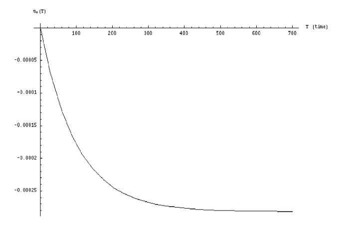
FIG. 1.: Mean velocity of the solitary wave due to a resonator impedance. Solitons decelerate at first due to the dissipative part of the wakefield. However, over long times, they approach a steady state where the wakefields have sufficiently decayed due to the finite resonator bandwidth.

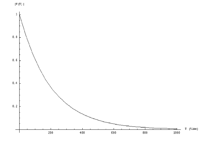
FIG. 2.: Voltage amplitude on the resonator. The voltage first grows due to the longitudinal impedance, followed by oscillations which result from the interference of energy between the solitary waves and the core of the beam. The envelope of the amplitude eventually decays as detuning occurs.

In Figs. 3 and 4 we show the corresponding mean velocity and voltage from a coasting beam simulation previously reported. The behavior is manifestly similar to that predicted by Eq. (35), (53) and (61) , though no attempt has been made to check the precise scaling of the physical quantities.

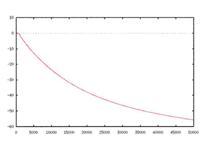
FIG. 3.: Mean velocity of the solitary waves from the simulation showing deceleration toward a fixed maximum energy separation. There is good qualitative agreement with the analytical result.

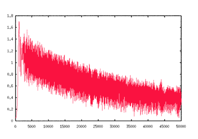
FIG. 4.: Voltage amplitude on the resonator from the particle simulation. There is good qualitative agreement between the analytical results and the voltage envelope shown.

IV Conclusions

In this work we have derived a set of equations for solitary waves on a coasting beam using a renormalization group approach. This procedure has led to a specific set of evolution equations in the practical case of a cavity resonator of finite Q. The resulting set of equations can be solved analytically under certain assumptions, and this leads to an explicit form for the soliton and its behavior over time. We find, in contrast to other solitary waves in the presence of dissipation, that solitons can persist over long times and do so by decelerating from the core of the beam. This deceleration leads to detuning and the decay of the driving voltage. The result is that a nearly steady state is reached, albeit with a gradually decreasing soliton strength, but fixed maximum energy separation.

Good qualitative agreement between the analytic results and the simulations have been observed. We note that such a process may well indicate a method by which well-defined droplets can occur in the halo of intense stored beams. Further study of this problem, and the application of the RG approach to bunched-beam evolution will be considered in future work.

V ACKNOWLEDGMENTS

The authors gratefully acknowledge the continuing support of D. Finley and S. Holmes for the pursuit of this erudite topic. The authors also gratefully acknowledge helpful discussions with Alejandro Aceves and Jim Ellison.

REFERENCES

• [1] R. Fedele, G. Miele, L. Palumbo and V.G. Vaccaro, ” Thermal Wave Model for Nonlinear Longitudinal Dynamics in Particle Accelerators,” Physics Letters A, 179, 407, (1993)
• [2] J.J. Bisognano, Solitons and particle beams, Particles and fields series 47, High Brightness Beams for Advanced Accelerator Applications, AIP Conference Proceedings 253, College Park MD, (1991).
• [3] L.-Y. Chen, N. Goldenfeld and Y. Oono, “Renormalization Group and Singular Perturbations: Multiple Scales, Boundary Layers, and Reductive Perturbation Theory,” Phys. Rev. E 54, 376, (1996).
• [4] T. Kunihiro, “The Renormalization Group Method Applied to Asymptotic Analysis of Vector Fields,” Prog. of Theoretical Physics, 97, 179 (1997).
• [5] M. Goldman, “Strong Turbulence of Plasma Waves,” Rev. of Modern Physics, 56, 709 (1984).
• [6] S. G. Thornhill, D. terHaar, “Langmuir Turbulence and Modulational Instability,” Physics Reports, 43, 43-99 (1978).
• [7] P. A. Robinson, “Nonlinear Wave Collapse and Strong Turbulence,” Rev. of Modern Physics, 69, 507 (1997).
• [8] V. E. Zakharov and A. B. Shabat, “Exact Theory of Two-Dimensional Self-Focussing and One-Dimensional Self-Modulation of Waves in Nonlinear Media,” Sov. Phys. JETP, 34, 62 (1972).
• [9] D. R. Nicholson and M. V. Goldman, “Damped Nonlinear Schroedinger Equation,” Phys. of Fluids, 19, 1621 (1976).
• [10] N. R. Pereira and L. Stenflo, “Nonlinear Schroedinger Equation Including Growth and Damping,” Phys. of Fluids, 20, 1733 (1977).
• [11] N. R. Pereira, “Solution of the Damped Nonlinear Schroedinger Equation,” Phys. of Fluids, 20, 1735 (1997).