The lid method for exhaustive exploration of metastable states of complex systems

Abstract

The ‘lid’ algorithm is designed for the exhaustive exploration of neighborhoods of local energy minima of energy landscapes. This paper describes an implementation of the algorithm, including issues of parallel performance and scalability. To illustrate the versatility of the approach and to stress the common features present in landscapes of quite different systems, we present selected results for 1) a spin glass, 2) a ferromagnet, 3) a covalent network model for glassy systems, and 4) a polymer. The exponential nature of the local density of states found in these systems and its relation to the ordering transition is briefly commented upon.

I Introduction

The state space $\bf{S}$ of a complex systems together with a scalar function $E:\bf{S}\rightarrow\bf{R}$, is often described as a ‘landscape’[1]. For discrete state spaces, a landscape is a graph, whose nodes represent the states and where edges connect neighbor states. Each node is characterized by a scalar function, $E$, which in physical systems is usually the energy of a state, while in other cases it can be a cost or a fitness. Often the system dynamics takes the form of a Markov process with states in the landscape and transitions among neighbors. In thermally activated processes hopping to states of higher energy is a very rare event at low temperatures. In this regime the system remains trapped for very long times within relatively small sets of states surrounding local energy minima. The relation between low temperature relaxation dynamics and the geometrical properties of the traps, which can be studied by the lid algorithm presented in this paper, is a topic of great current interest. Several theories for the behavior of complex systems at low temperature, e.g. aging, have been advanced[2, 3, 4, 5, 6], which build on assumptions about state space geometry. In chemistry, low-energy configurations of clusters[7, 8, 9, 10], proteins[11, 12], polymers[13] and solids[14, 15, 16] may represent metastable compounds, whose reaction pathways and lifetimes are of considerable importance. Finally, heuristic optimization techniques based on annealing [17] may benefit from any insight on generic properties of the low energy part of the landscapes [18].

The ‘lid’ algorithm provides exact geometrical information by exhaustively visiting subsets of state space, which are characterized by two quantities: a low energy ‘reference state’, $\psi$ , and a ‘lid’, $L$. The enumeration starts with $\psi$, and covers all those states which are connected to $\psi$ by paths never exceeding the energy level $L$. Clearly, the set of states registered, ${\cal P}_{\psi,L}$, henceforth called a ‘pocket’, is likely to behave as a dynamical trap in a thermal relaxation process. Roughly, one expects the trajectory to remain confined to the pocket for time scales of order $\exp(L/T)$, where $T$ is the temperature and the Boltzmann constant is set to one (the escape time may exceed this value considerably, if large entropic barriers are present[16]). If a deep pocket is metastable, it is possible to study the relaxation behavior in its interior (independently of the rest of the energy landscape), either at the microscopic level [19] or using a coarse-grained ”lumped” model of the pocket[20].

Following a discussion of the algorithm, we present selected results from four rather different applications. This demonstrates the versatility of the method and stresses the interesting - and not widely recognized fact - that important features of landscapes are common to rather different systems. A more detailed discussion of some of the examples can be found in separate publications[16, 21, 22]. Similarly, we refer to the literature for implementations and applications of the lid method to continuous (rather than discrete) landscapes[20, 23]. A different approach to the exploration of complex landscape based on branch and bound methods can be found in ref. [24].

II The lid method

To visualize how the lid method works, imagine water welling up at a local minimum $\psi$ of the landscape. For concreteness we take the energy of this state, $E(\psi)$, to be equal to zero. The height of the water level above $\psi$ then corresponds to the value of the lid $L$. Initially, $\psi$ will be the deepest point of a lake, but, eventually, another point $\psi^{\prime}$ with lower energy $E(\psi^{\prime})<E(\psi)$ might become submerged. If this happens, a watershed is crossed and the pocket containing $\psi^{\prime}$ is flooded. The smallest lid value at which the overflowing occurs defines the depth of the pocket centered at $\psi$.

The amount of landscape submerged, or volume, ${\cal V}_{\cal P}(L)$ provides a simple measure of the shape of the pocket as a function of the lid. Further information is provided by the height distribution of the submerged points, i.e., the local density of states ${\cal D}_{\cal P}(E;L)$, by the number of accessible minima, ${\cal M}_{\cal P}(L)$, and by their distribution ${\cal DM}_{\cal P}(E;L)$. Depending on the problem at hand, additional questions can be asked: what is the height of the lowest saddle which must be reached before the water can flow to the ‘sea’ - i.e. - before the flooded part of state space percolates. And how does this height scale with some important parameter of the problem - e.g. its size (number of atoms or spins) - or the value of an external field. All these properties are local, since they are independent of other properties of the landscape outside the pocket itself.

III The search algorithm

The application of the lid algorithm to a given problem involves task-dependent as well as task-independent procedures. To the former class belong the evaluation of the energy function, the implementation of the move class and the coding of the configurations. The task independent features are the generation and storage of the configurations, and their subsequent retrieval from a suitably organized data base. The link between the two types of tasks is the coding of the system configurations as binary strings. (Note that e.g. an Ising model is already naturally coded this way).

The purpose of the search is to enumerate all those states of the system which can be reached by repeated applications of elementary moves, starting at $\psi$ and without ever exceeding a preset value, $L$, of the energy. To understand how the enumeration works, one may identify three disjoint sets of states. The first set, A, consists of states which have been visited, and whose neighbors have all been visited. The second set, B, includes points which have been visited, but where not all the neighbors have been seen. Finally, the third set, C, includes all the accessible but as yet undiscovered points. Initially, B contains just one point - the reference state $\psi$, A is empty, and C contains a finite but unknown number of points. The program terminates when B and C are empty, or earlier, if a lower lying reference state is discovered during the search.

In principle the enumeration task can be accomplished using two data structures: 1) a data base containing the visited states, henceforth referred to as a ‘tree’ and 2) a linked list containing pointers to the elements of the data base. This list is later also referred to as a ‘buffer’. The data base is ordered according to the value of a tag, which is the value in base ten of the binary string encoding each configuration. The tree and the buffer will be collectively called a ‘search structure’.

The progress of the algorithm is given by a position marker along the list: states to the left of the marker are of class A, those to the right are of class B. The subroutine, generate, takes as its ‘current’ state the first available state of class B and calculates all its neighbors. This is done in several steps: First, the configuration is decoded, i.e. the actual configuration is calculated from the tag. Then the neighbors are created and their energy is computed. States above the lid are immediately discarded. If the system possesses translational or other symmetries, each of the remaining states must first be brought into a unique representative configuration. When this is done, the configuration is encoded into a binary string, whose tag is computed and then used to check the new configuration against states already found. When appropriate, the configuration is appended to the data base and a corresponding pointer is added to the linked list, to the immediate right of the current marker position, i.e. in class B. Upon return from generate, the current state is updated, by moving the pointer one step to the right along the list. Initially, the number of B states greatly increases. As the calculation progresses, fewer and fewer new states are found below the lid, and, finally, the search terminates when the current position of the marker reaches the end of the list.

In pseudo-code, the conceptual, if not the actual, structure of the (search part of the) algorithm is quite simple.

1. Read input data.

2. Initialize structures:

   1. Store reference configuration in binary search tree.

   2. Initialize the linked list buffer. The first and only record in the buffer has two elements: a pointer to the reference configuration and a null pointer. The latter will later point to the next element of the buffer.

   3. Initialize a pointer, current, to point to the first position in the buffer.

3. Generate neighbors to the current configuration.
   If current is not null:

   1. Create a list of all neighbor states of current configuration. Assign to each of these a unique tag.

   2. Remove from the list those neighbors which have energy above the lid.

   3. Remove from the list those states which have the same tag as states previously stored in the binary tree.

   else Exit the program.

4. Append to the binary tree and update the buffer:

   1. Append each new state to the binary tree, ordered according to the value of tag.

   2. For each append, insert a new record in the buffer, right after the ‘current’ position. The two elements of the record are a pointer to the configuration just appended, and a pointer to the next record in buffer.

5. Move the current pointer one step forward along the buffer.

6. Go to point 3.

In the actual implementation of the code it is important to minimize the number of malloc calls and of cache misses by allocating memory in large blocks. The parallel implementation of the code described in section IV is rather more complicated, but provides a substantial speed-up.

IV Parallel implementation

As the size of the data base which has to be managed by the lid algorithm can be considerable for large lids, i.e. up to hundreds or even thousands of Megabytes of RAM, there is a strong motivation to increase the speed of execution by parallelizing the search. A very coarse-grained parallelism, e.g. the simultaneous execution of multiple runs with different input parameter values is not a viable option due to the very large memory requirements. Two lower levels of parallelization were considered: 1) Generate the neighbors of each configuration in parallel, as described in point 3 of the algorithm in section III. 2) Define $N$ buffers and $N$ binary trees and perform the search and append procedure in parallel. As the first approach does not lead to any speed-up we shall concentrate on the second, which parallelizes quite successfully.

A Parallel structure

In order to balance the search load among $NP$ processors, each configuration is assigned a positive integer $ID$, with $0\leq$ $ID$ $<N$. Each $ID$ identifies a parallel thread, and each processor runs $NP/N$ threads. Each thread has its own buffer and search tree, which together constitute a search structure. To obtain a uniform distribution of the load across the processors, the values of the assigned $ID$’s should be uniformly distributed in the interval $[0,N]$. Within the above load-sharing scheme the scalability of the algorithm can be negatively affected by 1) the overhead for communication along $N(N-1)$ different channels, and 2) deviations from perfect internal load balance. Our analysis shows that the main detrimental effect stems from 2), at least for moderate values of $NP$.

The program initialization procedure is similar to the sequential case. All the $N$ search structures will initially be empty, except for the zero’th one, which must contain the reference state. The parallel program includes points 3) and 4) of the algorithm in section III as well as a supplementary part dealing with the communication among different threads. The need of communicating arises because the $ID$ of a configuration can differ from those of its neighbors. Hence, only a fraction of the newly generated states can be handled by the same thread as their parent. The rest is temporarily stored in a square array of linked lists $mail$, where $mail[i][j]$ contains states generated by thread $j$ which have to be handled by thread $i$.

All parallelism was implemented at a high level, using so called #pragma constructs [25]. These are ignored on a single processor machine, which makes the program easily portable to different architectures. The relevant parallel part of the code looks as follows:

while (	not_all_threads_idle)
{
	#pragma paral	lel (start parallel	region)
	{
		#pragma pfor (…..)
		for ( each thread i, i=0, … N)
		{
			get_from_mail	(read mail from other threads)
			s_search	(check if the received states are
				already present and update if needed )
			while ( more configurations are in buffer i )
			{
				for current	configuration:
				generate	( generates all the neighbors of current
					configuration, calling the following three procedures:
				create	(creates neighbor configurations and assigns their ID’s
					for the spin glass case, this routine is called
					flip )
				energy	(energy calculation - for spin glass called
					init_energy3D )
				s_search	(see above) )
			}
		}
		mp_end_pdo
		mp_barrier
		mp_barrier_nthreads
		#pragma one processor
		check if all threads are done
		mp_barrier
		mp_barrier_nthreads
	}
}

In the above fragment of pseudocode, all routines starting with ”mp” are not user written. Calls to these routines from the SGI thread library are inserted by the compiler to steer the parallelization. The #pragma parallel construct causes the ‘for-loop’ to be executed in parallel. After completion of the ‘while-loop’, all threads are synchronized again. Then, one of the threads checks whether the algorithm is finished or not, and sets a shared flag accordingly. In this way, all other threads will be notified about the current status, and either continue with their ‘while-loop’ or terminate. In addition to this explicit parallelism, a lock is used to implement the earlier mentioned ”mail” mechanism, which enters in the routine get_from_mail. Basically, each thread monitors a specific memory location, in order to check for any incoming states. If there are such states, the thread will raise a flag (to stop new mail from flowing in), empty the mail queue with the states into a memory location which it owns, reset the flag and continue.

B Parallel performance analysis

To assess the efficiency of the parallel implementation, we first ported the program to a Silicon Graphics Origin2000 system with MIPS R10000 processors running at 250MHz[26]. This machine has a 64 bit shared memory architecture i.e. the entire address space is accessible to all threads. We mainly used the spin-glass model for the tests, since it has an easily evaluated energy function and hence a lower one-processor load and a higher communication load relative to the glass and polymer problem. The parallel scalability of most other problems is expected to be higher than the spin-glass case.

In the spin glass tests, the length of the parallel ‘for-loop’ was $16$ and the number of processors was varied from $1$ to $16$. Two series of runs were performed, with the lid value set to $0.038$ and to $0.046$ respectively. The corresponding memory requirements were $200$ Mbytes and $2$ Gbytes.

Table I lists the elapsed times in seconds together with two parallel speed-up metrics, for the test case with the smallest lid. We have used the uniprocessor elapsed time as a reference. Under column ”Rel. Speed-up” we list the speed-up obtained when doubling the number of processors. Ideally this number should be $2$. Under column ”Cum. Speed-up” we define the speed-up on $P$ processors to be $T(1)/T(P)$. In the ideal case this should be $P$. The last column contains the estimated performance using Amdahl’s law[27]. Briefly, Amdahl’s law assumes that the uni-processor elapsed time $T(1)$ can be split in an optimizable and a non-optimizable part, say: $T(1)=fT(1)+(1-f)T(1)$, where $f$ is the fraction of the time that can benefit from optimization (which in our case is achieved through parallelism). The elapsed time $T(P)$ on $P$ processors is then $T(P)=(f/P)T(1)+(1-f)T(1)$. By measuring $T(1)$ and $T(2)$ the equation can be solved for $f$, whence $T(P)$ can be (crudely) estimated for any $P$. In our case the procedure yields $f=0.81$.

As can be seen, the simple Amdahl model severely underestimates the performance, probably due to the anomalous behavior with $2$ processor as further discussed in the sequel. The parallel performance was analyzed in more detail using the IRIX SpeedShop profiling environment [28]. Among other things, this tool gives the elapsed time for every function executed by each thread, thus clarifying the scalability of different parts of the program. The results are presented in Table II. The function s_search does not appear in this table because it was inlined by the compiler. Since a run with a lid value of $0.038$ constitutes a rather small job, where the parallelization overhead can be relatively dominant, we also ran the program for a lid value of $0.046$ requiring slightly more than $2$GB of main memory. The relative timings, plus associated metrics, are listed in table III. As expected, we achieve a higher parallel efficiency for this problem size. And, again, Amdahl’s law strongly underestimates the performance for the large processor numbers. In table IV we list the profile information obtained on 1, 2 4, 8 and 16 processors. The speed-up values for the user routines are given in table V. These routines account for 99% of the total computation time on a single processor. The corresponding speed-up values are given in table V. One observes that the user routines parallelize rather well albeit not perfectly. Also, the routines do not scale by the same factor, which of course limits the overall scalability of the program. As expected, the function get_from_mail, which implements the exchange of (a rather small amount of) data among the $N$ threads is the poorest performer in terms of scalability, as the costs of locking the mailbox must become dominant for high $N$.

From table IV we observe that the cost of the pragma generated barrier function decreases from its maximum at $N=2$. The SpeedShop profiler was also used to analyze which part of the program is actually responsible for the heavy usage of the barrier function. It was found to be in the parallelized for-loop i.e. the first barrier construct in the code fragment shown above is mainly responsible for the times given in table IV. The same type of behavior appears more clearly in the performance of the lid algorithm on the network glass model described in sectionV C. Unlike the spin-glass model, the energy evaluation and the coding-decoding of the string representation of a configuration are computationally demanding. Indeed, the eight most time consuming routines perform these very tasks. The elapsed times in seconds and the other metrics are listed in TableVI. For reasons that will be explained below, and in contrast with previous estimates, we have used $T(1)$ and $T(4)$ to estimate the fraction of parallelized code entering the Amdahl rule. As is clear from the data, the performance on 2 processors sticks out in a negative way, even though a profile of the user routines (not included), shows that these scale perfectly. The fact that the cost of the barrier reaches a peak for $2$ processors probably stems from an imbalance in the workload assigned by the algorithm to each processor: As all processors are synchronized at the barrier located at the end of the parallelized for loop, the slowest processor sets the overall pace. Arguably, the imbalance increases with the workload per processor and the cost of synchronization is highest when the load per processor peaks. For fixed total load this happens at $NP=2$, as observed. As a further check we performed tests for a series of increasing lids (i.e. increasing total workloads) and found a systematic deterioration of the parallel performance with two processors, but no negative effects with eight processors. Finally, we note that the second of the compiler inserted barriers, which is located at the end of the one processor section of the code, has a minimal impact on scalability. This is because the processors, having just been synchronized by the previous barrier, spend very little time at this part of the code.

In summary, we see that: 1) for a spin-glass problem with $16$ threads the shortest turnaround time is obtained on $16$ processors, but the best parallel efficiency on $8$ processors. 2) Due to some non-scalable parts in the program, a slight load imbalance within the algorithm and the cost of synchronization itself, the scalability of the program is not perfect. However, on a medium sized production problem, the current implementation still achieves a speed-up of up to $9.3$ on $16$ processors. Scalability is slightly better on the more computation intensive glass problem. In general, we expect that on larger problems and on problems with a higher one-processor load, the parallel efficiency will improve further. As the cost of synchronization seems quite substantial, high latency networks (typically a cluster of machines) would probably not handle this type of problems efficiently. A more asynchronous implementation of the algorithm is likely to reduce idle time and further enhance scalability. The SGI parallel environment does provide means to implement this, but the possibility has not yet been investigated by the authors.

V Applications

To illustrate the versatility of the lid algorithm, and highlight the presence of common features across different systems, we briefly discuss four applications. A detailed discussion of the physics is given in Ref. [21] for the spin glass case, in Ref. [22] for the 2d-network case, and finally in Ref.[16] for the polymer case. Here we just stress the observation that the scale parameter of the exponential growth of e.g. the local density of states can be identified with the temperature where the trap looses its thermal metastability. In some cases, (e.g. the spin-glass and the ferromagnetic models) this temperature turns out to be quite close to the actual critical temperature of the system.

A Spin glass

A set of $\cal N$ Ising spins, $\sigma_{i}=\pm 1$, is placed on a 3D cubic lattice with periodic boundary conditions. The energy of the $x$’th configuration, $0<x\leq 2^{\cal N}$, is defined by the well known Hamiltonian[29]

$$E(x)=-\frac{1}{2}\sum_{i,j}J_{ij}\sigma_{i}(x)\sigma_{j}(x),$$ (1)

where $J_{ij}=J_{ji}$ and where $J_{ij}\neq 0$ only if spins $i$ and $j$ are adjacent on the grid. In this case, and for $i<j$,  we take the $J_{ij}$’s as independent gaussian variables, with zero average and variance $J^{2}=1$. This last choice fixes the (dimensionless) energy and temperature scales. Neighbor configurations are by definition those which differ in the orientation of exactly one spin. As an example, we show in figure 1 a the local density of states ${\cal D}(E,L_{max})$ for 25 realizations of the $J_{ij}$’s on the $5^{3}$ lattice. We notice that ${\cal D}(E,L_{max})$ exhibits a rather simple behavior, growing almost exponentially, with a systematic downward curvature. In a semilogarithmic plot the curvature is fully accounted for by a parabola, which has a very small second order term. The density of states is for convenience normalized to one within the pocket. The raw data are indicated by plusses and the full lines are fits of the logarithm of $\cal{D}$ to a parabola. The second order term obtained in the fit is of the order of $1/50$ of the linear term. Similarly, the available volume in the pocket is also close to an exponential function of the lid energy, if one disregards the jumps which occur whenever a new ‘side pocket’ is accessed as the barrier increases.

B Ferromagnetic Ising model

The Hamiltonian of the ferromagnetic Ising model has the same form as Eq. 1, except for the crucial fact that the non-zero $J_{ij}$ are all identical and equal to one. Again, neighbor configurations differ by one spin flip. This model’s landscape can hardly be considered as complex: it has two global energy minima, i.e. the ground states where all the spins are aligned, and no local energy minima. The lid algorithm was applied to the problem in order to see whether the known critical temperature could be predicted from the form of the local density of states. The latter quantity is depicted in figure 1 b for a $7\times 7$, an $8\times 8$ and a $4\times 4\times 4$ lattice. Remarkably, there is in all cases an exponential growth. The energy scales characterizing it are $2.66$, $2.70$ and $4.66$, respectively, which compare favorably with the true critical temperatures: $2.27$ in $2d$[30] and $\approx 4.51$ in $3d$[31].

C Structural glass (2d)

A random network of ‘atoms’ placed on a 2D square lattice[16, 22] can serve as a model for covalent glasses[32]. The energy of a configuration of the network is the sum of two-body- and three-body-potential terms. The former has a repulsive term for short distances $r<2d$, where $d$ is the lattice spacing, and an attractive term, which reaches zero smoothly for $r>3.2d$. The three-body-potential prevents bond angles below $80^{\circ}$, and introduces a preferred bond angle, which is $\approx 120^{\circ}$. Thus, the global minimum configuration would be a network consisting of hexagons. To avoid surface effects, periodic boundary conditions are applied. Neighbor configurations are created by shifting the position of one atom by one lattice unit. Each bit of the binary string encoding a configuration represents the state of one lattice site. Its value is one if the site is occupied, and zero otherwise.

The energy landscapes of the networks were investigated for a range of densities and sizes of the simulation cell. We show in figure 1 c a typical example of $27$ atoms on a $14\times 14$ lattice. The figure depicts the accessible phase space volume ${\cal V}(L)$ and the number of accessible minima ${\cal M}(L)$, together with the local density of states ${\cal D}(E;L)$, and density of minima ${\cal DM}(E;L)$, in a pocket enclosing a deep local minimum of the energy landscape. We note that all these quantities show an approximately exponential growth with the lid $L$ and the energy $E$, respectively.

D Polymer glass (2d)

As a final example we mention random polymers on a two-dimensional lattice. The energy function is similar to that of the network model, except for two features: The polymers are not allowed to break up or grow in size, i.e. $V(r)=\infty$ for $r>3.2$, and the interaction between atoms not occupying consecutive positions along a polymer is purely repulsive for $r<1.6$, and zero otherwise.

As the monomers have fixed positions along different polymers, the encoding of a configuration is more involved: each lattice point has a fixed number, and each monomer is assigned the binary value of the position it occupies in a given configuration. These short binary strings are appended to one another, in the order of the building units of the polymer. This procedure creates the long binary string used to identify the whole configuration. In figure 1 d, we show as one specific example, the phase space volume ${\cal V}(L)$, the number of accessible minima ${\cal M}(L)$, the local density of states ${\cal D}(E;L)$ and the density of minima ${\cal DM}(E;L)$ for a system of two polymers of length $18$ on a $14\times 14$ lattice. We observe that the pocket in the landscape for these (relatively long) polymers also exhibits exponential growth in the above quantities as a function of $L$ and $E$, respectively.

VI Summary and Discussion

In this paper we have presented a rather general algorithm for the exhaustive exploration of subsets of states (pockets) in complex energy landscapes. Such an exhaustive exploration can be used to map out the low energy part of energy landscape, yielding information which e.g. helps understanding the low-temperature relaxation behavior of the systems. We have analyzed the program’s parallel performance, and demonstrated its applicability to four different physical applications, which required a relatively large computational effort.

The lid approach may complement more traditional Monte Carlo simulations as an exploratory tool: it yields complete information on energetic barriers, but is, by construction, insensitive to entropic barriers, e.g. bottlenecks between various parts of the landscape which should all be ”accessible” during relaxation at low temperatures if only energetic barriers were relevant.

It is interesting to note that the landscapes of the rather different applications considered share a key feature: the fact that the local density of states within typical pockets is approximately exponential. The energy scale of this exponential identifies the temperature at which the trap looses its thermal metastability[18, 19, 21]. In several instances this temperature is also close to an actual transition temperature. It thus appears that exponential local densities of state within traps may be part of the mechanism behind e.g. the spin glass and glass transitions[21, 22].

As computers get faster and memory less expensive, it is our hope that the lid algorithm will help to uncover the landscape structure of many different complex systems, leading to a better understanding of e.g. the dynamics of relaxations and phase transitions for such systems.

Acknowledgments The authors would like to thank the Silicon Graphics Advanced Technology Centre in Cortaillod (Switzerland) for making the Origin2000 system available to the project and Statens Naturvidenskabelige Forskningråd for providing part of the computer resources and for travel grants. P.S. is indebted to Richard Frost of the San Diego Supercomputing Center for good advice on parallel computing, and C. S. would like to thank the DFG for funding via SFB408 and a Habilitation stipend.

Processors	Elapsed time	Rel. speed-up	Cum. speed-up	Amdahl time
1	848	1.00	1.00	(848)
2	506	1.68	1.68	(504)
4	298	1.70	2.85	(333)
8	169	1.76	5.02	(247)
16	115	1.47	7.37	(204)

TABLE I.:

Origin2000 performance for the 3-d spin-glass; lid value $L=0.038$.

Function	# Processors
	1	2	4	8	16
$generate$	479.3	247.9	130.9	69.5	38.3
$get\_from\_mail$	263.7	132.9	68.5	39.5	39.5
$init\_energy3D$	102.9	52.1	26.5	13.3	6.6
$flip$	7.4	4.2	2.3	1.4	0.9
$mp\_barrier\_nthreads$	0.0	53.7	51.7	37.4	28.1
Cumulative time	853.3	490.2	279.9	161.1	113.4

TABLE II.:

Origin2000 performance breakdown at the function level for the 3-d spin-glass; lid value $L=0.038$.

Processors	Elapsed time	Rel. speed-up	cum. speed-up	Amdahl time
1	12535	1.00	1.00	(12535)
2	7288	1.72	1.72	(7287)
4	3914	1.86	3.20	(4664)
8	2218	1.76	5.65	(3352)
16	1342	1.65	9.34	(2696)

TABLE III.:

Origin2000 performance for the 3-d spin-glass; lid value $L=0.046$.

Function	Processors
	1	2	4	8	16
$generate$	5685	3006	1552	811	435
$get\_from\_mail$	5708	3650	1590	811	520
$init\_energy3D$	1085	544	272	139	70
$flip$	95	54	31	17	11
$mp\_barrier\_nthreads$	0	443	436	374	237
Cumulative time	12573	7697	3881	2152	1273

TABLE IV.:

Origin2000 performance breakdown at the function level for the 3-d spin-glass; lid value $L=0.046$.

Function	Processors
	1	2	4	8	16
$generate$	1.00	1.89	3.66	7.01	13.07
$get\_from\_mail$	1.00	1.56	3.59	7.04	10.98
$init\_energy3D$	1.00	1.99	3.99	7.81	15.50
$flip$	1.00	1.76	3.06	5.59	8.64

TABLE V.:

Parallel speed-up values for the 3-d spin-glass; lid value $L=0.046$.

Processors	Elapsed time	Rel. speed-up	Cum. speed-up	Amdahl time
1	14011	1.00	1.00	(14011)
2	10486	1.34	1.34	(7664)
4	4455	2.35	3.15	(4490)
8	2025	2.20	6.92	(2903)

TABLE VI.:

Origin2000 performance for 2-d network model; lid value $L=4.2(eV/atom)$.

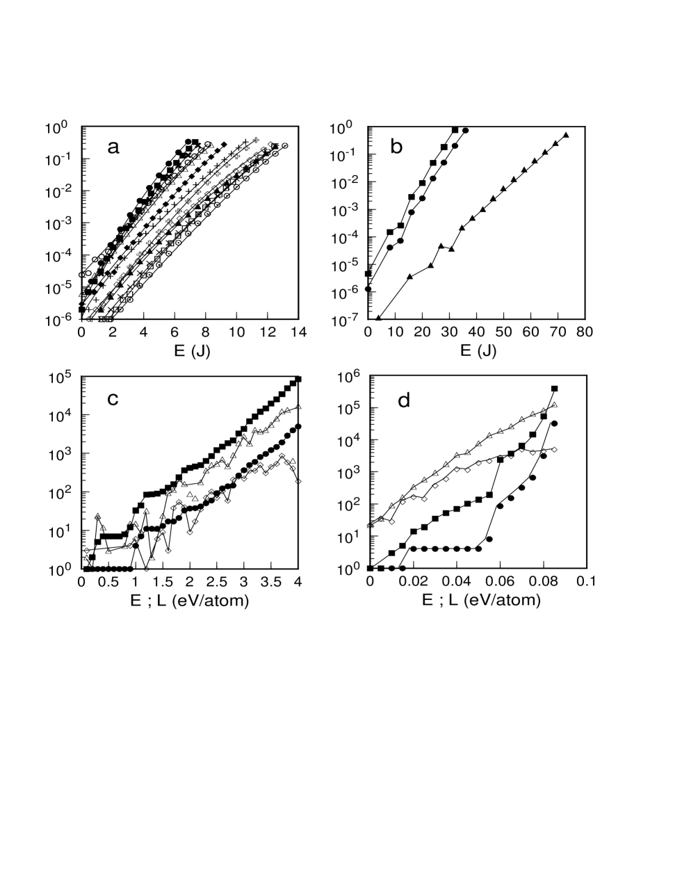
FIG. 1.:

Plate a) shows the local densities of states ${\cal D}(E,L_{max})$ for 12 realizations of the $J_{ij}$’s of a spin-glass model on a $5^{3}$ lattice. Plate b) shows the same quantity for the ferromagnetic Ising model. The circles are for a $8\times 8$ lattice, the squares for $7\times 7$ lattice and the triangles for a $4\times 4\times 4$ lattice. In all cases the data are divided by the total number of states found, which is seen to be of the order of one million. The abscissa is the total energy in units of $J$. For the spin glass $J$ is the standard deviation of the distribution of the couplings and the ferromagnet it is the coupling constant itself. The scale of the exponential growth parameter averaged over $25$ different realizations (13 data sets are omitted to avoid cluttering the graphics) is $T_{c}=0.6$ for the spin glass model. In the ferromagnetic case we find and $T_{c}\approx 2.7$ in the two dimensional lattices, and $T_{c}\approx 4.7$ in three dimensions. These figures are close to the transition temperatures of the corresponding systems, which are $T_{c}\approx 0.84$ for the spin glass, $T_{c}=2.27$ for the two-dimensional ferromagnet and and $T_{c}\approx 4.51$ for the three dimensional one. Plates c) and d) show data for the 2d network model of a glass and for the polymer system, respectively. The abscissa is either the energy $E$ or the lid $L$, both in (eV/atom). The curves are : the available volume ${\cal V}(L)$ (squares) and the number of minima ${\cal M}(L)$ (circles) as a function of the lid; the local density of states ${\cal D}(E,L_{max})$ (triangles) and the local density of minima ${\cal DM}(E,L_{max})$ (diamonds) as a function of the energy.

REFERENCES

- [1] Landscape paradigms in Physics and Biology, Hans Frauenfelder, Alan R. Bishop, Angel Garcia, Alan Perelson, Peter Schuster, David Sherrington and Peter J. Swart Eds. Physica D 107, Nos. 2-4, 1996
- [2] K. H. Hoffmann and P. Sibani. Phys. Rev. A 38, (1988), 4261
- [3] P. Sibani and K. H. Hoffmann. Phys. Rev. Lett. 63, (1989), 2853
- [4] J. P. Bouchaud. J. Phys. I France 2, (1994), 139
- [5] Jorge Korchan and Laurent Laloux. J. Phys. A: Math. Gen. 29, (1996), 1929
- [6] P. Sibani and K. H. Hoffmann. Physica A 234, (1997), 751
- [7] R. S. Berry. Chem. Rev. 93, (1993), 2379
- [8] R. S. Berry. J. Phys. Chem. 98, (1994), 6910
- [9] R. E. Kunz and R. S. Berry. Phys. Rev. E 49, (1994), 1895
- [10] D. J. Wales. Science 271, (1996), 925
- [11] C. M. Dobson, A. Sali, M. Karplus. Angew. Chem. Int. Ed. Engl. 37, (1998), 868
- [12] J. N. Onuchic, Z. Luther-Schulten, P. G. Wolynes. Annu. Rev. Phys. Chem. 48, (1997), 539
- [13] O. M. Becker and M. Karplus. J. Chem. Phys. 106, (1997), 1495
- [14] J. C. Schön and M. Jansen. Angew. Chem. Int. Ed. Engl. 35, (1996), 4001
- [15] H. Putz, J. C. Schön and M. Jansen. J. Comp. Mater. Sci. 11, (1998), 309
- [16] J. C. Schön. Habilitation Thesis., Univ. Bonn, 1997
- [17] A. Möbius, A. Neklioudov, A. Díaz-Sánchez, K. H. Hoffmann, A. Fachat and M. Schreiber. Phys. Rev. Lett. 79, (1997), 4297
- [18] J. C. Schön. J. Phys. A 30 (1997), 2367
- [19] P. Sibani, J. C. Schön, P. Salamon and J.-O. Andersson. Europhys. Lett. 22, (1993), 479. P. Sibani and P. Schriver. Phys. Rev B 49:6667, 1994
- [20] J. C. Schön, H. Putz and M. Jansen. J. Phys.:Cond. Matter. 8, (1996), 143
- [21] P. Sibani. to appear in Physica A 1998.
- [22] J. C. Schön and P. Sibani. to appear in J. Phys. A 1998.
- [23] J. C. Schön. Ber. Bunsenges. Phys. Chem. 100, (1996), 1388
- [24] T. Klotz, S. Schubert and K. H. Hoffmann. cond-mat preprint 9710146
- [25] Silicon Graphics Inc, C Language Reference Manual, Document Number 007-0701-120, 1998
- [26] SiliconGraphics Inc., Origin Servers, SGI Technical Report, April 1997.
- [27] G.M. Amdahl, in Proc. AFIPS 1967 Spring Joint Computing Conference, Vol.30, page 483-485, AFIPS Press, Reston, VA, 1967
- [28] Silicon Graphics Inc, SpeedShop User’s Guide, Document Number 007-3311-002, 1998
- [29] S. F. Edwards and P. W. Anderson. J. Phys. F 5, (1975), 89
- [30] Shang-Keng Ma. Statistical Mechanics , World Scientific, 1985
- [31] C. Domb, in Phase Transitions and Critical Phenomena, Vol. 3, C. Domb and M. S. Green Eds. Academic Press, New York, 1974
- [32] W. H. Zachariasen. J. Amer. Chem.Soc. 54 (1932), 3841