ON THE MECHANISM OF FORMATION OF THE EFIMOV STATES IN THE HELIUM ⁴He TRIMER

Abstract

A mechanism of disappearance and formation of the Efimov levels of the helium ⁴He trimer is studied when the force of the interatomic interaction is changed. It is shown that these levels arise from virtual levels which are in turn formed from (quasi)resonances settled on the real axis. The resonances including virtual levels are calculated by the method based on the solution of the boundary value problem, at complex energies, for the Faddeev differential equations describing the scattering processes $(2+1\to 2+1;\,1+1+1)$. All the calculations are performed with the known interatomic Aziz He – He -  potential HFD-B. A very strong repulsive component of this potential at short distances between helium atoms is approximated by a hard core. A special attention is paid to the substantiation of the method used for computing resonances and to the investigation of its applicability range.

I Introduction

The ⁴He three-atomic system is of considerable interest in various fields of physical chemistry and molecular physics. Studies of the helium dimer and trimer represent an important step towards understanding the properties of helium liquid drops, superfluidity in ⁴He films, and so on (see, for instance, Refs. [1, 2, 3]). Besides, the helium trimer is probably a unique system where a direct manifestation of the Efimov effect  [4] can be observed since the binding energy $\epsilon_{d}$ of the ⁴He dimer is extremely small ($\sim-1$ mK [5, 6, 7]) even in the molecular scale. For this reason, the helium trimer is certainly of interest for nuclear physicists, too. Moreover a theoretical study of the ⁴He trimer is based just on the same methods of the theory of few-body systems that are used in solving three–body nuclear problems.

From the standpoint of the general theory of few–body systems, the ⁴He trimer belongs to three–body systems that are most difficult for a specific investigation, first, owing to its Efimov nature, and second, because it is necessary to take into account the practically hard core in the interatomic He – He - interaction  [8, 9, 10, 11]. At the same time the problem of three helium atoms can be considered as an example of an ideal three–body quantum problem since the ⁴He atoms are identical neutral bosons with zero spin and the analysis of this problem is complicated neither by separation of spin–isospin variables nor by taking into account the Coulomb interaction.

There is a great number of experimental and theoretical studies of ⁴He clusters. However, most of the theoretical investigations consist merely in computing the ground-state energies of clusters of that sort, mainly on the basis of variational methods [12, 13, 14, 15, 16]. Besides, the methods based on hyperspherical expansions of the Schrödinger and Faddeev equations [17, 18, 19] in the coordinate representation were used. Also, the Faddeev integral equations in the momentum representation were employed in Refs. [20, 21] while the results of Ref. [22] are based on a direct solving the two-dimensional Faddeev differential equations in configuration space. From the experimental studies we would like to mention those of Refs. [5, 6, 7, 23] where clusters consisting of a small number of noble gase atoms were investigated.

Though much effort was undertaken for studying molecular clusters various problems related to the ⁴He trimer remained beyond the scope of thorough consideration. In particular, the elastic scattering phases of a helium atom on a helium dimer and breakup amplitudes (at ultralow energies) have been calculated only recently [24, 25, 26]. These computations were preceded only by the computation of characteristics of the He–He₂ scattering at zero energy [20] and estimation of the recombination rate $(1+1+1\to 2+1)$ [27].

As a matter of fact, we have already pointed out basic reasons for computations of excited states and scattering being especially difficult in the ⁴He₃ system. First, this is a low energy of the dimer $\epsilon_{d}$ which necessitates to consider very large domains in the configuration space with a characteristic size of hundreds of Å. Second, a very strong repulsive component in the He–He interaction produces large errors in the standard approximation of the three–atomic Hamiltonian at short distances between atoms. The capacities of modern computers do not yet allow one to reach dimensions of grids that would remove both the above-mentioned reasons and would provide stable results with the use of the conventional methods.

The present paper is a sequel of studies of the ⁴He₃ system undertaken in the papers [24, 25, 26] within an approach that is capable, as we think, to resolve both the above-mentioned numerical problems. In these papers the repulsive component of the He–He interaction at short distances between atons is approximated by a hard core. This allows one to investigate the ⁴He₃ system within a mathematically rigorous method of solving a three-body problem in the Boundary-Condition Model developed in [28, 29]. An important advantage of such an approach that essentially diminishes computational errors is the necessity to approximate, inside the core domains, only the Laplacian operator instead of the sum of this operator and a huge repulsive components of the He – He - potentials (see [26]). In [24, 25, 26], such an approach has been successfully applied for calculating not only scattering but also binding energies of the ground and excited states of the helium trimer. Investigation made in  [24, 25, 26] has shown that the method proposed in [28, 29] is well suited for performing three–body molecular computations in the case where repulsive components of interatomic interactions are of a hard core nature.

There is a series of works [18, 21, 26] showing that the excited state of the ⁴He trimer is initiated indeed by the Efimov effect  [4]. In these works the various versions of the Aziz ⁴He–⁴He potential were employed (HFDHE2 [8], HFD-B [9], and LM2M2 [10]). However, the basic result of Refs. [18, 21, 26] on the excited state of the helium trimer is the same: this state disappears when the interatomic potential is multiplied by the “amplification factor” $\lambda$ of order 1.2. More precisely, if this potential is multiplied by the increasing factor $\lambda>1$ then the following effect is observed. First, the difference $\epsilon_{d}(\lambda)-E_{t}^{(1)}(\lambda)$ between the dimer energy $\epsilon_{d}(\lambda)$ and the energy of the trimer excited state $E_{t}^{(1)}(\lambda)$ increases. Then the behavior of this difference radically changes and with further increase of $\lambda$ it monotonously decreases. At $\lambda\approx 1.2$ the level $E_{t}^{(1)}$ disappears. It is just such a nonstandard behavior of the energy $E_{t}^{(1)}(\lambda)$ as the coupling between helium atoms becomes more and more strengthening, points to the Efimov nature of the trimer excited state. And vice versa, when $\lambda$ slightly decreases (no more than 2 %), the second excited state $E_{t}^{(2)}$ appears in the trimer [18, 21].

This paper is aimed at elucidating the fate of the trimer excited state upon its disappearance in the physical sheet when $\lambda>1$ and at studying the mechanism of arising of new excited states when $\lambda<1$. As the interatomic He – He potential, we use the potential HFD-B [9]. We have established that for such He – He - interactions the trimer excited level $E_{t}^{(1)}$ merges with the threshold $\epsilon_{d}$ at $\lambda\approx 1.18$ and with further decreasing $\lambda$ it transforms into a virtual level of the first order (a simple real pole of the analytic continuation of the scattering matrix) lying in the unphysical energy sheet adjoining the physical sheet along the spectral interval between $\epsilon_{d}$ and the three–body threshold. We trace the position of this level for $\lambda$ increasing up to 1.5. Besides, we have found that the excited (Efimov) levels for $\lambda<1$ also originate from virtual levels of the first order that are formed in pairs. Before a pair of virtual levels appears, there occurs a fusion of a pair of conjugate resonances of the first order (simple complex poles of the analytic continuation of the scattering matrix in the unphysical sheet) resulting in the virtual level of the second order.

As it will be clear from the further exposition (see Sect. III), the above-mentioned resonances are not, generally speaking, genuine resonances of the ⁴He₃ trimer since they are situated outside of the energy domain for which we can rigorously prove the applicability of the method we are using for computing the resonances. We will call the resonances found outside the range of guaranteed applicability of the method the (quasi)resonances.

The paper is organized as follows.

In Sect. II, we describe the method of search for resonances in a three–body system on the basis of the Faddeev differential equations. The idea of the method consists in calculating the analytic continuation of the component ${\rm S}_{0}(z)$ (see formula (6)) of the scattering matrix corresponding to the ($2+1\to 2+1$) process, in the physical sheet with the use of these equations. A particular attention in this section is paid to the description of the parabolic domain on the physical sheet where one can analytically continue the function ${\rm S}_{0}(z)$ by numerical solving the coordinate space Faddeev partial equations. For the potentials we use, the three–body resonances (including virtual levels) lying in the unphysical sheet of energy $z$ plane adjoining the physical sheet along the interval $(\epsilon_{d},0)$ are the roots of the function ${\rm S}_{0}(z)$ in the physical sheet. We have earlier employed this method for computing resonances as roots of ${\rm S}_{0}(z)$ in the three–nucleon problem [30].

In Sect. III, we first briefly describe the numerical method we use to solve the $(2+1\to 2+1;\,1+1+1)$ scattering problem for the ⁴He₃ system with going out into the domain of complex energies. Then we describe the results of our calculations.

Some notation used throughout the paper is as follows: by ${\mathbb{C}}$ we denote the complex plane; $\sqrt{z}$ stands for the main branch of the function $z^{1/2}$, $\mathop{\rm Im}\sqrt{z}\geq 0$ for any $z\in{\mathbb{C}}$; the symbol ${\mathbb{R}}^{2}_{+}$ is used for the quadrant $x\geq 0$, $y\geq 0$; by $L_{2}({\mathbb{R}}^{2}_{+})$ we understand the Hilbert space of complex–valued functions which are integrable on ${\mathbb{R}}^{2}_{+}$ with the absolute value squared; the symbol $\overline{z}$ stands for the complex number conjugated to $z$.

II Method for search of resonances in a three–body system on the basis of the Faddeev differential equations

A Faddeev partial differential equations in the case of smooth potentials

In this paper, we will consider the ⁴He₃ system in the state with the total angular momentum $L=0$.

First we consider the case where the interatomic interactions are described by conventional smooth potentials that include no hard-core component. In this case, the angular partial analysis reduces the initial Faddeev equation for three identical bosons to a system of coupled two-dimensional integro-differential equations [31]

$$\left[H_{0,l}-z\right]F_{l}(x,y)=-V(x)\Psi_{l}(x,y)\,.$$ (1)

Here, $x,y$ stand for the standard Jacobi variables, $x\geq 0$ and $y\geq 0$, and

$$H_{0,l}=-\displaystyle\frac{\partial^{2}}{\partial x^{2}}-\displaystyle\frac{\partial^{2}}{\partial y^{2}}+l(l+1)\left(\displaystyle\frac{1}{x^{2}}+\displaystyle\frac{1}{y^{2}}\right)\,$$ (2)

for the partial component of the kinetic energy operator. Functions from the domain of $H_{0,l}$ are assumed to obey the boundary conditions

$$F_{l}(x,y)\left.\right|_{x=0}=0\,,\qquad F_{l}(x,y)\left.\right|_{y=0}=0\,.$$ (3)

which are quite standard when the expansions over bispherical basis are used. The potential $V(x)$ is assumed to be central. In our paper, the energy $z$ can get both real and complex values. At $L=0$ the partial angular momentum $l$ corresponds both to the dimer and an additional atom. The momentum $l$ can assume only even values, $l=0,2,4,\ldots\,.$

The partial wave functions $\Psi_{l}(x,y)$ are expressed through the Faddeev partial components $F_{l}(x,y)$ by the relations

$$\Psi_{l}(x,y)=F_{l}(x,y)+\sum_{l^{\prime}}\int_{-1}^{+1}d\eta\,h_{ll^{\prime}}(x,y,\eta)\,F_{l^{\prime}}(x^{\prime},y^{\prime})\,$$ (4)

where

$$x^{\prime}=\sqrt{\displaystyle\frac{1}{4}\,x^{2}+\displaystyle\frac{3}{4}\,y^{2}-\displaystyle\frac{\sqrt{3}}{2}\,xy\eta}\,,\qquad y^{\prime}=\sqrt{\displaystyle\frac{3}{4}\,x^{2}+\displaystyle\frac{1}{4}\,y^{2}+\displaystyle\frac{\sqrt{3}}{2}\,xy\eta}\,,$$

and $-1\leq{\eta}\leq 1$. The explicit form of the functions $h_{ll^{\prime}}$ can be found, e. g., in Refs. [31, 32] (see also [26]). Here we only deal with a finite number of equations (1), assuming that $l\leq l_{\rm max}$ where $l_{\rm max}$ is a certain fixed even number, $l_{\rm max}\geq 0$. The condition $0\leq l\leq l_{\rm max}$ is equivalent to the supposition that the potential $V(x)$ only acts in the two-body states with $l=0,2,\ldots,l_{\rm max}$. The spectrum of the Schrödinger operator for a system of three identical bosons with such a potential is denoted by $\sigma_{3B}$.

Its is well known (see, e. g., Ref. [31]) that if the potential $V(x)$ is smooth and decreasing as $x\to\infty$ together with its derivatives not slower than $x^{-3-\varepsilon}$, $\varepsilon>0$, then the asymptotic conditions as $\rho\rightarrow\infty$ and/or $y\rightarrow\infty$ for the partial Faddeev components of the $(2+1\rightarrow 2+1\,;\,1+1+1)$ scattering wave functions for $z=E+{\rm i}0$, $E>0$, read

$$\begin{array}[]{rcl}F_{l}(x,y;z)&=&\delta_{l0}\psi_{d}(x)\left\{\sin(\sqrt{z-\epsilon_{d}}\,y)+\exp({\rm i}\sqrt{z-\epsilon_{d}}\,y)\left[{\rm a}_{0}(z)+o\left(1\right)\right]\right\}\\ &&+\displaystyle\frac{\exp({\rm i}\sqrt{z}\rho)}{\sqrt{\rho}}\left[A_{l}(z,\theta)+o\left(1\right)\right]\,.\end{array}$$ (5)

We assume that the ⁴He₂ dimer has an only bound state with an energy $\epsilon_{d}$, $\epsilon_{d}<0$, and wave function $\psi_{d}(x)$. This function is assumed to be normalized so that for all $x>0$ values of $\psi_{d}(x)$ are real. The notations $\rho$, $\rho=\sqrt{x^{2}+y^{2}}$ , and $\theta$, $\theta=\mathop{\rm arctg}\displaystyle\frac{y}{x}$ , are used for the hyperradius and hyperangle. The coefficient ${\rm a}_{0}(z)$, $z=E+{\rm i}0$, for $E>\epsilon_{d}$ is the elastic scattering amplitude. The functions $A_{l}(E+{\rm i}0,\theta)$ provide us, at $E>0$, the corresponding partial Faddeev breakup amplitudes. Note that for $z=E+{\rm i}0$ the correction terms $o(1)$ in coefficients of outgoing waves $\exp({\rm i}\sqrt{z-\epsilon_{d}}\,y)$, $E>\epsilon_{d}$, and $\exp({\rm i}\sqrt{z}\rho)/\sqrt{\rho}$, $E>0$, in (5) are of the form, respectively, $o(y^{-1/2})$ and $o(\rho^{-1/2})$. This property ensures uniqueness of the solution of the boundary value problem (1 – 5) for real scattering energies $E>\epsilon_{d}$ [31].

The $(2+1{\rightarrow}2+1)$ component of the $s$-wave partial scattering matrix for a system of three helium atoms is given for real $z=E+{\rm i}0$, $E>\epsilon_{d}$, by the expression

$${\rm S}_{0}(z)=1+2{\rm i}{\rm a}_{0}(z)\,$$ (6)

while the $(2+1\to 2+1)$ scattering phases read

$$\delta_{0}(p)=\frac{1}{2}\,{\rm Im}\,\ln{\rm S}_{0}(\epsilon_{d}+p^{2}+{\rm i}0)\,,\quad p>0,$$

where $p$ stands for the momentum conjugated to the Jacobi variable $y$.

B Holomorphy domains of the Faddeev components $F_{l}(z)$ and scattering matrix ${\rm S}_{0}(z)$

Our goal is to study the analytic continuation of the scattering matrix ${\rm S}_{0}(z)$ into the complex plane (the physical sheet). As it follows from the results of Refs. [33, 34], roots of the function ${\rm S}_{0}(z)$ in the physical sheet of energy $z$ plane correspond to the location of the three-body resonances situated in the unphysical sheet connected with the physical sheet by crossing the spectral interval $(\epsilon_{d},0)$. This statement is a particular case of more general statements regarding the three-body resonances obtained in [33, 34] for the case of two-body potentials decreasing in the coordinate space not slower than exponentially. We assume that $V(x)$ is just a potential which falls off exponentially and, thus, for all $x\geq 0$

$$|V(x)|\leq C\exp(-\mu x)\,,$$ (7)

with some positive $C$ and $\mu$. For the sake of simplicity we even assume sometimes that $V(x)$ is finite, i. e., $V(x)=0$ for $x>r_{0}$, $r_{0}>0$. Looking ahead, we note that, in fact, in our numerical computations of the ⁴He₃ system at complex energies we make a “cutoff” of the interatomic He – He - potential at a sufficiently large radius $r_{0}$.

It is well known that different representations of the same holomorphic function (for instance, either by a series or by an integral) allow one to describe this function only in some parts of its Riemann surface. The description [33, 34] of the holomorphy domains for different truncations of the total three-body scattering matrix in the physical sheet was based on the use of the Faddeev integral equations in the momentum representation. In this paper, we make use of the Faddeev equations in the configuration space. Therefore it is necessary to perform an investigation, independent of [33, 34], of domains in the physical sheet where we can analytically continue the Faddeev components $F_{l}(x,y;z)$ and the amplitudes ${\rm a}_{0}(z)$ and $A_{l}(z,\theta)$ just with the use of the configuration space techniques.

Let us list briefly the main results of this investigation obtained by us for the ⁴He₃ system under the assumption (7). To formulate these results we distinguish the following three domains in the complex plane ${\mathbb{C}}$.

1^∘. The domain $\Pi^{(\Psi)}$ where the Faddeev components $F_{l}(x,y;z)$ (and, hence, the wave functions $\Psi_{l}(x,y;z)$) can be analytically continued in $z$ so that the differences

$$\Phi_{l}(x,y;z)=F_{l}(x,y;z)-\delta_{l0}\psi_{d}(x)\sin(\sqrt{z-\epsilon_{d}}\,y)$$ (8)

at $z\in\Pi^{(\Psi)}\setminus\sigma_{3B}$ turn out to be elements of $L_{2}({\mathbb{R}}_{+}^{2})$. The domain $\Pi^{(\Psi)}$ is described by the inequality

$$\mathop{\rm Im}\sqrt{z-\epsilon_{d}}<{\rm min}\left\{\frac{\sqrt{3}}{2}\mu,\,\sqrt{3}\sqrt{|\epsilon_{d}|}\right\}\,.$$ (9)

For fixed $x,y$ the functions $\Phi_{l}(x,y;z)$ are continuous in $z$ up to the rims of the cut along the continuous spectrum $[\epsilon_{d},+\infty)$.

2^∘. The domain $\Pi^{(A)}$ where both the elastic scattering amplitude ${\rm a}_{0}(z)$ and the Faddeev breakup amplitudes $A_{l}(z,\theta)$ can be analytically continued in $z$, $z\not\in\sigma_{3B}$, provided that the functions $F_{l}(x,y;z)$ obey the asymptotic formulas (5). This domain is described by the inequalities

$$\mathop{\rm Im}\sqrt{z}+\frac{1}{2}\mathop{\rm Im}\sqrt{z-\epsilon_{d}} < \frac{\sqrt{3}}{2}\sqrt{|\epsilon_{d}|}\,,$$ (10)

$$\mathop{\rm Im}\sqrt{z}+\mathop{\rm Im}\sqrt{z-\epsilon_{d}} < \frac{\sqrt{3}}{2}\mu\,.$$ (11)

3^∘. And finally, we distinguish the domain $\Pi^{(S)}$, most interesting for us, where the analytic continuation in $z$, $z\not\in\sigma_{3B}$, can be only done for the elastic scattering amplitude ${\rm a}_{0}(z)$ (and consequently, for the scattering matrix ${\rm S}_{0}(z)$); the analytic continuabilty of the amplitudes $A_{l}(z,\theta)$ in the whole domain $\Pi^{(S)}$ is not required. The set $\Pi^{(S)}$ is a geometric locus of points obeying the inequality

$$\mathop{\rm Im}\sqrt{z-\epsilon_{d}}<\mathop{\rm min}\left\{\frac{1}{\,\sqrt{3}\,}\,\sqrt{|\epsilon_{d}|},\,\frac{\,\sqrt{3}\,}{2}\mu\right\}\,.$$ (12)

For the domains $\Pi^{(\Psi)}$, $\Pi^{(A)}$, and $\Pi^{(S)}$, the following chain of inclusions

$$\Pi^{(A)}\subset\Pi^{(S)}\subset\Pi^{(\Psi)}.$$

is valid.

Note that the type (9) or (12) condition,

$$\mathop{\rm Im}\sqrt{z-a}<\sqrt{b},\qquad a\in{\mathbb{R}},\,b>0,$$ (13)

is equivalent to the inequality

$$\mathop{\rm Re}z>a-b+\frac{1}{4b}\,(\mathop{\rm Im}z)^{2}\,.$$ (14)

Therefore, for $\mu\leq 2\sqrt{|\epsilon_{d}|}$ the set $\Pi^{(\Psi)}$ is the domain bounded by the parabola

$$\mathop{\rm Re}z>-|\epsilon_{d}|-\frac{3}{4}\mu^{2}+\frac{1}{3\mu^{2}}(\mathop{\rm Im}z)^{2}\,.$$ (15)

For $\mu>2\sqrt{|\epsilon_{d}|}$ this set coincides with the domain

$$\mathop{\rm Re}z>-4|\epsilon_{d}|+\frac{1}{12|\epsilon_{d}|}(\mathop{\rm Im}z)^{2}\,.$$ (16)

Analogously, if $\mu\leq\frac{2}{3}\sqrt{|\epsilon_{d}|}$ then the domain $\Pi^{(S)}$ is described by the inequality (15); whereas for $\mu>\frac{2}{3}\sqrt{|\epsilon_{d}|}$ by the inequality

$$\mathop{\rm Re}z>-\frac{\,4\,}{3}|\epsilon_{d}|+\frac{3}{4|\epsilon_{d}|}(\mathop{\rm Im}z)^{2}\,.$$ (17)

As to the curves bounding the domains (10) and (11), we only notice that their order with respect to the variables $\mathop{\rm Re}z$ and $\mathop{\rm Im}z$ is higher than the second order. It is easy to check that each of these curves is connected, symmetric with respect to the $\mathop{\rm Re}z$ axis and crosses the latter only once. For the first curve this intersection occurs at $z=\frac{3}{4}\epsilon_{d}$, the slope angle of the tangent at the point of intersection being independent of $\epsilon_{d}$, $\frac{d\mathop{\rm Re}z}{d\mathop{\rm Im}z}\biggr{|}_{\mathop{\rm Im}z=\pm 0}=\pm\frac{\sqrt{3}}{2}$. As $\mathop{\rm Re}z\to+\infty$, the boundaries (10) and (11) are asymptotically approximated by the type (14) parabolas with coefficients $a$ and $b$ which can be computed explicitly.

To prove the assertion 1^∘ concerning the domain $\Pi^{(\Psi)}$ we note that the functions $\Phi_{l}(x,y;z)$ given by the formulas (8) satisfy the equations

$$\left[H_{0,l}+V(x)-z\right]\Phi_{l}(x,y;z)+V(x)\sum_{l^{\prime}}\int_{-1}^{+1}d\eta\,h_{ll^{\prime}}(x,y,\eta)\,\Phi_{l^{\prime}}(x^{\prime},y^{\prime},z)=\chi_{l}(x,y;z)\,$$ (18)

where

$$\chi_{l}(x,y;z)=-V(x)\int_{-1}^{+1}d\eta\,h_{l0}(x,y,\eta)\psi_{d}(x^{\prime})\sin(\sqrt{z-\epsilon_{d}}\,y^{\prime})\,.$$

Obviously, for $z\in\Pi^{(\Psi)}$ the functions $\chi_{l}(x,y;z)$ fall off exponentially as $\rho\to\infty$. Moreover, for all the directions $0\leq\theta\leq\pi/2$ the uniform estimate

$$\chi_{l}(x,y;z)\mathop{\mbox{$=$}}\limits_{\rho\to\infty}O\biggl{(}\exp(-\alpha\rho)\biggr{)}\,$$

is valid with $\alpha={\rm min}\left\{\frac{\sqrt{3}}{2}\mu-\mathop{\rm Im}\sqrt{z-\epsilon_{d}},\,\frac{\sqrt{3}}{2}\sqrt{|\epsilon_{d}|}-\frac{1}{2}\mathop{\rm Im}\sqrt{z-\epsilon_{d}}\right\}\,.$ Consequently, if the condition (9) holds then the inhomogeneous terms $\chi_{l}(x,y;z)$ considered as functions of the variables $x$ and $y$ at fixed $z$, are elements of $L_{2}({\mathbb{R}}^{2}_{+})$. At the same time, the vectors $\chi_{l}(z)$ turn out to be holomorphic functions of $z\in\Pi^{(\Psi)}$ with respect to the $L_{2}({\mathbb{R}}^{2}_{+})$ norm.

In the problem under consideration, the spectrum of the Faddeev matrix operator defined by the l.h.s. of Eqs. (18) and by the boundary conditions (3) in the Hilbert space constituted of the vectors $\Phi=(\Phi_{0},\Phi_{2},\ldots,\Phi_{l_{\rm max}})$, $\Phi_{l}\in L_{2}({\mathbb{R}}^{2}_{+})$, coincides with the spectrum $\sigma_{3B}$ of the corresponding three-boson Schrödinger operator with two-body potentials $V(x)$ only acting in the states with $l=0,2,\ldots,l_{\rm max}$. This means that for any energy $z\in\Pi^{(\Psi)}$ lying outside of the spectrum $\sigma_{3B}$, the inhomogeneous system (18) is uniquely solvable in the class of the functions $\Phi_{l}(z)\in L_{2}({\mathbb{R}}^{2}_{+})$, $l=0,2,\ldots,l_{\rm max}$. Since outside of the set $\sigma_{3B}$ the resolvent of the Faddeev operator is a holomorphic operator-valued function of the variable $z$, each of the components $\Phi_{l}(z)$ of the solution of Eqs. (18) also is a holomorphic function of $z\in\Pi^{(\Psi)}\setminus\sigma_{3B}$. The bound-state energies of the three-boson system under consideration turn out to be poles of the first order for $\Phi_{l}(z)$. Thus, the Faddeev partial components $F_{l}(x,y;z)$ admit the analytic continuation in $z$ in the form (8) into the domain $\Pi^{(\Psi)}\setminus\sigma_{3B}$.

The proof of the assertions of  2^∘ and 3^∘ regarding the domains $\Pi^{(S)}$ and $\Pi^{(A)}$ is rather cumbersome. This is why we here only outline its main steps. Note that the proof is based on the integral equations method and it is quite standard (see, for instance, Ref. [31], Chapter V). First, the equations (18) are rewritten in the form of the Faddeev partial integral equations. To do this, it suffices to reverse the operators $H_{0,l}+V-z$ in (18). Since the variables $x$ and $y$ in $H_{0,l}$ are separated, the kernels $R^{(l)}_{v}(X,X^{\prime};z)$, $X=\{x,y\}$, $X^{\prime}=\{x^{\prime},y^{\prime}\}$, of the respective resolvents $R^{(l)}_{v}(z)=(H_{0,l}+V-z)^{-1}$ are explicitly expressed in terms of the two-body problem. Analytic properties in the variable $z$ and coordinate asymptotics of the kernels $R^{(l)}_{v}(X,X^{\prime};z)$ are well known (see Ref. [31], Chapters IV and V). Iterations first “improve” and then stabilize the asymptotic properties of the iterated kernels and inhomogeneous terms of the Faddeev equations. (In the case under consideration, this stabilization requires only three iterations.) Further, it turns out that, for $z\not\in[\epsilon_{d},+\infty)$, the iterated kernels are represented by sums of exponentially decreasing terms admitting, in certain domains of the configuration space, an explicit asymptotic factorization with respect to $X$ and $X^{\prime}$. Since we are working in the domain where $\chi_{l}(z)\in L_{2}({\mathbb{R}}^{2}_{+})$, the corresponding asymptotic factors of these terms, along with the asymptotics of the iterations of the inhomogeneous term, determine the coordinate asymptotics of the functions $\Phi_{l}(x,y;z)$. Therefore, finally we are able to determine the geometric locus of the points $z$ in the complex plane for which there exists a (non-empty) set in the configuration space such that the leading term of the coordinate asymptotics of the function $\Phi_{l}(x,y;z)$ in this set represents a term of the form ${\rm a}_{0}(z)\psi_{d}(x)\exp({\rm i}\sqrt{z-\epsilon_{d}}\,y)$, and thus, for these $z$ the scattering matrix ${\rm S}_{0}(z)$ is well defined. This geometrical locus is just the domain $\Pi^{(S)}$. In this domain, as $y\to\infty$ and/or $\rho\to\infty$, the functions $\Phi_{l}(x,y;z)$ admit the asymptotic representation

$$\Phi_{l}(x,y;z) = \delta_{l0}\psi_{d}(x)\left\{\exp({\rm i}\sqrt{z-\epsilon_{d}}\,y)\left[{\rm a}_{0}(z)+o(1)\right]+{\rm f}_{0}(y;z)\right\}$$ (19)

$$+ \displaystyle\frac{\exp({\rm i}\sqrt{z}\rho)}{\sqrt{\rho}}\left[A_{l}(z,\theta)+o(1)\right]+{\rm F}_{1,l}(x,y;z)$$ (20)

with

$${\rm f}_{0}(y;z)\mathop{\mbox{$=$}}\limits_{y\to\infty}O\left({\rm e}^{-\alpha_{0}(z)y}\right)\qquad\mbox{and}\qquad{\rm F}_{1,l}(x,y;z)\mathop{\mbox{$=$}}\limits_{\rho\to\infty}O\left({\rm e}^{-\alpha_{1}(z)\rho}\right)\,$$ (21)

where

$$\alpha_{0}(z) = \frac{\sqrt{3}}{2}\,\sqrt{|\epsilon_{d}|}-\frac{\,1\,}{2}\,\mathop{\rm Im}\sqrt{z-\epsilon_{d}}\,,$$ (22)

$$\alpha_{1}(z) = \mathop{\rm min}\left\{\alpha_{0}(z)\,,\,\,\frac{\sqrt{3}}{2}\,\mu-\mathop{\rm Im}\sqrt{z-\epsilon_{d}}\,,\,\mathop{\rm Im}\sqrt{z}\right\}\,.$$ (23)

In a parabolic neighborhood of the $y$-axis, the functions ${\rm F}_{1,l}(x,y;z)$ are also subjected to the asymptotic estimates

$${\rm F}_{1,l}(x,y;z)\mathop{\mbox{$=$}}\limits_{\begin{array}[]{c}y\to\infty\\ x<y^{\nu}\end{array}}O\biggl{(}\exp(-\alpha_{0}(z)y)\biggr{)}\,$$ (24)

where $\nu$ is an arbitrary fixed number smaller than unity, $\nu<1$.

As to the domain $\Pi^{(A)}$, the leading asymptotic term of each of the functions ${\rm F}_{1,l}(x,y;z)$ for $z\in\Pi^{(A)}$ is a spherical wave $\exp({\rm i}\sqrt{z}\rho)/\sqrt{\rho}$ with the amplitude $A_{1,l}(\theta)$ being a differentiable function of the angle $\theta$. Therefore, for $z\in\Pi^{(S)}$ the term ${\rm F}_{1,l}(x,y;z)$ in the r.h.s. of the formula (19) can be added to the asymptotic term with a spherical wave preceding ${\rm F}_{1,l}$. In the domain $\Pi^{(S)}$, and hence, in a narrower domain $\Pi^{(A)}$ the condition ${\rm f}_{0}(y;z)\mathop{\mbox{$=$}}\limits_{y\to\infty}o\biggl{(}\exp({\rm i}\sqrt{z-\epsilon_{d}}\,y)\biggr{)}\,$ holds. Consequently, for $z\in\Pi^{(A)}$, the Faddeev components $F_{l}(x,y;z)$ do obey the standard asymptotic conditions like (5).

Therefore, for any $\nu<1$ the dominant term of the asymptotics of the function $\Phi_{0}(x,y;z)$, $z\in\Pi^{(S)}\setminus\sigma_{3B}$, in the domain $x<y^{\nu}$ reads as ${\rm a}_{0}(z)\psi_{d}(x)\exp({\rm i}\sqrt{z-\epsilon_{d}}\,y)$ as $y\to\infty$. This means that, for $z\in\Pi^{(S)}\setminus\sigma_{3B}$, it is always possible by solving the equations (1) to separate explicitly the elastic scattering amplitude ${\rm a}_{0}(z)$ and, thus, to construct the analytic continuation of the scattering matrix ${\rm S}_{0}(z)$.

Outside of the domain $\Pi^{(S)}$ the numerical construction of ${\rm S}_{0}(z)$ by solving the Faddeev differential equations is, in general, impossible since for $x<y^{\nu}$ and $\nu<1$ both functions ${\rm f}_{0}(y;z)$ and ${\rm F}_{1,0}(x,y;z)$, $z\not\in\Pi^{(S)}$, include terms decreasing slower than $\exp({\rm i}\sqrt{z-\epsilon_{d}}\,y)$ as $y\to\infty$.

C The partial Faddeev differential equations in the case of potentials with hard core

In the case of potentials with hard core, the partial Faddeev differential equations for a system of three identical bosons at $L=0$ acquire the form

$$\left[H_{0,l}-z\right]F_{l}(x,y)=\left\{\begin{array}[]{cl}-V(x)\Psi_{l}(x,y),&x>c\\ 0,&x<c\,,\end{array}\right.$$ (25)

where $c$, $c>0$, is the core size. The partial wave functions $\Psi_{l}(x,y)$ are expressed via Faddeev partial components $F_{l}(x,y)$ by the formulas (4). The components $F_{l}(x,y)$ satisfy the standard boundary conditions (3). The two-body central potential $V(x)$ acts only beyond the core domain, i. e. only where $x>c$. We assume as before that $V(x)$ falls off not slower than exponentially as $x\to\infty$ and, hence, it satisfies the condition (7) for some $C>0$ and $\mu>0$.

A main difference between the model with hard core and those with smooth potentials is that the functions $F_{l}(x,y)$ in this model satisfy the auxiliary boundary conditions

$$F_{l}(c,y)+\sum_{l^{\prime}}\int_{-1}^{+1}d\eta\,h_{ll^{\prime}}(c,y,\eta)\,F_{l^{\prime}}(x^{\prime},y^{\prime})=0\,$$ (26)

requiring that the wave functions $\Psi_{l}(x,y)$ vanish on the boundary $x=c$ of the core domain. It can be shown that in fact the conditions (26) force the wave functions (4) to vanish also inside the core domain at all energies except for a certain countable set of real values of $z$ (see Ref. [26] and references therein).

Asymptotic conditions for the partial Faddeev components $F_{l}(x,y;z)$ of the $(2+1\rightarrow 2+1\,;\,1+1+1)$ scattering wave functions as $\rho\rightarrow\infty$ and/or $y\rightarrow\infty$ are again of the form (5). The only difference is that the dimer wave function $\psi_{d}(x)$ is considered as zero in the core domain, i. e. for $0\leq x\leq c$.

In the hard-core model, all the assertions of Sect. II B regarding the holomorphy domains of the functions $\Phi_{l}(x,y;z)$ and the scattering matrix ${\rm S}_{0}(z)$ in $z$ still hold true.

D Resonances and virtual levels as roots of the scattering matrix ${\rm S}_{0}(z)$ in the physical sheet

We have already noticed that the roots of ${\rm S}_{0}(z)$ in the physical sheet of energy $z$ plane correspond to the location of the three-body resonances in the unphysical sheet adjoining the physical sheet along the spectral interval $(\epsilon_{d},0)$. In the case under consideration, this statement is an immediate consequence of the unitarity of the scattering matrix ${\rm S}_{0}(z)$ for $z=E+{\rm i}0$, $\epsilon_{d}\leq E\leq 0$,

$${\rm S}_{0}(E+{\rm i}0)\,\overline{{\rm S}_{0}(E+{\rm i}0)}=1\,.$$ (27)

Indeed, as we have established, the functions $\Phi_{l}(x,y;z)$ are holomorphic functions of $z\in\Pi^{(\Psi)}\setminus\sigma_{3B}$. Since the boundary value problem (1 – 5) is uniquely solvable, one easily verifies that the boundary values $\Phi_{l}(x,y;E+{\rm i}0)$ and $\Phi_{l}(x,y;E-{\rm i}0)$ for these functions on the rims of the cut along $[\epsilon_{d},+\infty)$ are related to each other as

$$\Phi_{l}(x,y;E+{\rm i}0)=-\overline{\Phi_{l}(x,y;E-{\rm i}0)}\,$$ (28)

since, on the one hand, their asymptotics (19) as $y\to\infty$ and/or $\rho\to\infty$ has the same structure and, on the other hand,

$$\chi_{l}(x,y;E+{\rm i}0)=-\chi_{l}(x,y;E-{\rm i}0)=-\overline{\chi_{l}(x,y;E-{\rm i}0)}\,,$$

since

$$\sin(\sqrt{E-\epsilon_{d}+{\rm i}0}\,y)=-\sin(\sqrt{E-\epsilon_{d}-{\rm i}0}\,y)=-\overline{\sin(\sqrt{E-\epsilon_{d}-{\rm i}0}\,y)}\,.$$

Consequently,

$${\rm a}_{0}(E+{\rm i}0)=-\overline{{\rm a}_{0}(E-{\rm i}0)}\,$$ (29)

and

$${\rm S}_{0}(E+{\rm i}0)=\overline{{\rm S}_{0}(E-{\rm i}0)}\,,\qquad E>\epsilon_{d}\,.$$ (30)

Therefore, it follows from Eq. (27) that for $\epsilon_{d}\leq E\leq 0$

$${\rm S}_{0}(E+{\rm i}0)=[{\rm S}_{0}(E-{\rm i}0)]^{-1}\qquad\mbox{and}\qquad{\rm S}_{0}(E-{\rm i}0)=[{\rm S}_{0}(E+{\rm i}0)]^{-1}\,.$$

This means that the function ${\rm S}_{0}(E+{\rm i}0)$ is continued through the cut $[\epsilon_{d},0]$ into the domain $\mathop{\rm Im}z<0$ as ${\rm S}_{0}^{-1}(z)$. In a similar manner, ${\rm S}_{0}(E-{\rm i}0)$ is continued into the domain $\mathop{\rm Im}z>0$, again as ${\rm S}_{0}^{-1}(z)$. All this signifies that the scattering matrix ${\rm S}_{0}(z)$ admits analytic continuation at least into the domain $\Pi^{(S)}$ of the unphysical energy sheet connected with the physical sheet by crossing the interval $[\epsilon_{d},0]$, the value of the continued function ${\rm S}_{0}(z)$ at $z\in\Pi^{(S)}$ in the unphysical sheet coinciding with the value of ${\rm S}_{0}^{-1}(z)$ at the same $z$ but in the physical sheet.

Recall that those points $z$ on unphysical sheets are called resonances where the analytically continued scattering matrix possesses poles. The resonances $z$ with zero imaginary part $\mathop{\rm Im}z=0$ and $\mathop{\rm Re}z<\epsilon_{d}$ are called the virtual levels.

Thus, we have here presented a simple proof of the fact that the resonances including the virtual levels corresponding to poles of the analytic continuation of the scattering matrix ${\rm S}_{0}(z)$ in the unphysical sheet connected with the physical one by crossing the spectral interval $[\epsilon_{d},0]$ are the roots of this matrix in the physical sheet. At the same time, the poles of the function ${\rm S}_{0}(z)$ in the physical sheet correspond to bound states of the three-boson system under consideration.

Concluding the subsection, we note that it follows from Eq. (29) that ${\rm a}_{0}(z)=-\overline{{\rm a}_{0}(\overline{z})}$ and, hence,

$$\overline{{\rm S}_{0}(z)}={{\rm S}_{0}(\overline{z})}$$ (31)

for any $z\in\Pi^{(S)}$. This means that the roots of the function ${\rm S}_{0}(z)$ are situated symmetrically with respect to the real axis.

III Numerical method and results of computations

In the present work we make use of the Faddeev equations (25) considered together with the boundary conditions (3), (5) and (26) to calculate the values of the ⁴He₃ scattering matrix ${\rm S}_{0}(z)$ in the physical sheet. We search for the resonances including the virtual levels as roots of ${\rm S}_{0}(z)$ and for the bound-state energies as positions of poles of ${\rm S}_{0}(z)$. All the results presented below are obtained for the case $l_{\rm max}=0$.

In all our calculations, $\hbar^{2}/m=12.12$ K Ų. As the interatomic He – He - interaction we employed the widely used semiempirical potential HFD-B constructed by R. A. Aziz and co-workers [9]. This potential is of the form

$$V_{\rm HFD-B}(x)=\varepsilon\left\{A\exp(-\alpha\zeta+\beta\zeta^{2})-\left[\frac{C_{6}}{\zeta^{6}}+\frac{C_{8}}{\zeta^{8}}+\frac{C_{10}}{\zeta^{10}}\right]F(\zeta)\right\}\,$$ (32)

where $\zeta=x/r_{m}$. The function $F(\zeta)$ reads

$$F(\zeta)=\cases{\exp{\left[-\left(D/\zeta-1\right)\right]^{2}},&\mbox{if $\zeta\leq D$}\cr 1,&\mbox{if $\zeta>D$}\,.}$$

For completeness the parameters of the potential HFD-B are given in Table I.

The value of the parameter $c$ (the core “diameter” of particles) is chosen to be so small that its further decrease does not appreciably influence the dimer binding energy $\epsilon_{d}$ and the energy of the trimer ground state $E_{t}^{(0)}$. Unlike papers [24, 25, 26], where $c$ was taken to be equal 0.7 Å, now we take $c=1.3$ Å. We have found that such a value of $c$ provides at least six reliable figures of $\epsilon_{d}$ and three figures of $E_{t}^{(0)}$.

Since the statements of Sect. II are valid, generally speaking, only for the potentials decreasing not slower than exponentially, we cut off the potential HFD-B setting $V(x)=0$ for $x>r_{0}$. We have established that this cutoff for $r_{0}\gtrsim 95$ Å provides the same values of $\epsilon_{d}$ ($\epsilon_{d}=-1.68541$ mK), $E_{t}^{(0)}$ ($E_{t}^{(0)}=-0.096$ K) and phases $\delta_{0}(p)$ which were obtained in our earlier calculations [24, 25, 26] performed with the potential HFD-B. Comparison of these results with results of other researchers can be found in Refs. [24, 25, 26]. In all the calculations of the present work we take $r_{0}=100$ Å. Note that if the formulas from Sect. II including the parameter $\mu$ are used for finite potentials, one should set $\mu=+\infty$.

Before making numerical approximation of the system of equations (3), (25), (26) at $l_{\rm max}=0$ we rewrite it in terms of a new unknown function $\Phi_{0}(x,y;z)$ that is expressed via the Faddeev component $F_{0}(x,y;z)$ by the relation (8). Note that for $z\in\Pi^{(\Psi)}\setminus\sigma_{3B}$ the function $\Phi_{0}(x,y;z)$ is square integrable in $x,y$ (see Sect. II B). Therefore, this function is uniquely determined by the asymptotic condition

$$\Phi_{0}(x,y;z)\mathop{\longrightarrow}\limits_{\rho\to\infty}0\,$$ (33)

that can be easily approximated and programmed. One could, for instance, require $\Phi_{0}(x,y;z)\biggr{|}_{\sqrt{x^{2}+y^{2}}=\rho_{\rm max}}=0$ at a sufficiently large $\rho_{\rm max}$ and look for a numerical solution of the system (3), (25), (26) satisfying this condition. Further, for $z\in\Pi^{(S)}$, one could, going sufficiently far from $\rho_{\rm max}$ into the domain of smaller (but nevertheless, providing the asymptotics (19)) values of $\rho$, separate the elastic scattering amplitude ${\rm a}_{0}(z)$, putting, e. g., ${\rm a}_{0}(z)\approx\Phi_{0}(x,y;z)\exp(-{\rm i}\sqrt{z-\epsilon_{d}}\,y)$, where the value of $x$ corresponds to the maximum of the function $\psi_{d}(x)$. Such an approach is, however, not effective in view of a relatively slow decrease of the exponentials $\exp(-\sqrt{|\epsilon_{d}|}\,x)$ and $\exp(-\mathop{\rm Im}\sqrt{z-\epsilon_{d}}\,y)$ as well as of the function $\exp(-\mathop{\rm Im}\sqrt{z}\,\rho)$ in the energy domain of interest for us in $\Pi^{(S)}$. For a proper approximation of the condition (33), very large values of $\rho_{\rm max}$ are to be taken. This is just a reason why one should take into account the asymptotics of the function $\Phi_{0}(x,y;z)$ as $x\to\infty$ and/or $y\to\infty$. Though the asymptotic formula (5) only holds for $z\in\Pi^{(A)}$, we employ it also for $z\in\Pi^{(S)}\setminus\Pi^{(A)}$. Indeed, when $z\in\Pi^{(S)}\setminus\Pi^{(A)}$, the leading term of the asymptotics of $\Phi_{0}(x,y;z)$ as $y\to\infty$ and $x<y^{\nu}$, $\nu<1$, is given by the same expression ${\rm a}_{0}(z)\exp({\rm i}\sqrt{z-\epsilon_{d}}\,y)$ (see Sect. II B) as in Eq. (5). Outside of the parabola $x<y^{\nu}$, it suffices to require the condition (33) to be satisfied. The presence, in Eq. (5), of the spherical wave $\exp({\rm i}\sqrt{z}\,\rho)/\sqrt{\rho}$ does not contradict this requirement. Therefore, the use of asymptotic condition (5) is justified even if $z\in\Pi^{(S)}\setminus\Pi^{(A)}$.

A detailed description of the numerical method we use is presented in Ref. [26]. Here we only mention main steps of the computational scheme [26] helpful for understanding our results.

When solving the boundary-value problem (3), (5), (25), (26) written in terms of the function $\Phi_{0}$, we carry out its finite-difference approximation in polar coordinates $\rho$ and $\theta$. The grid is chosen in such a way that the points of intersection of arcs $\rho=\rho_{i}$, $i=1,2,\ldots,N_{\rho}$, and rays $\theta=\theta_{j}$, $j=1,2,\ldots,N_{\theta}$, with the line $x=c$ turn out automatically to be its knots. The $\rho_{i}$ points are chosen according to the formulas

$$\rho_{i} = \frac{i}{N_{c}^{(\rho)}+1}\,c,\quad i=1,2,\ldots,N_{c}^{(\rho)},$$ (34)

$$\rho_{i+N_{c}^{(\rho)}} = \sqrt{c^{2}+y_{i}^{2}},\quad i=1,2,\ldots,N_{\rho}-N_{c}^{(\rho)},$$ (35)

where $N_{c}^{(\rho)}$ stands for the number of arcs inside the core domain and

$$y_{i}=f(\tau_{i})\sqrt{\rho^{2}_{N_{\rho}}-c^{2}},\quad\tau_{i}=\frac{i}{N_{\rho}-N_{c}^{(\rho)}}.$$

The nonlinear monotonously increasing function $f(\tau)$, $0\leq\tau\leq 1$, satisfying the conditions $f(0)=0$ and $f(1)=1$ is chosen in the form

$$f(\tau)=\left\{\begin{array}[]{lcl}\alpha_{0}\tau&,&\tau\in[0,\tau_{0}]\\ \alpha_{1}\tau+\tau^{\nu}&,&\tau\in(\tau_{0},1]\end{array}\right..$$

The values of $\alpha_{0}$, $\alpha_{0}\geq 0,$ and $\alpha_{1}$, $\alpha_{1}\geq 0,$ are determined via $\tau_{0}$ and $\nu$ from the continuity condition for $f(\tau)$ and its derivative at the point $\tau_{0}$. As a rule, we took values of $\tau_{0}$ within 0.1 and 0.2. The value of the power $\nu$ depends on the cutoff radius $\rho_{\rm max}=\rho_{N_{\rho}}=50\,$—$\,4100\,{\AA}$ its range being within 2 and 4 in our calculations.

The knots $\theta_{j}$ at $j=1,2,\ldots,N_{\rho}-N_{c}^{(\rho)}$ are taken according to $\theta_{j}=\mathop{\rm arctg}(y_{j}/c)$. The rest knots $\theta_{j}$, $j=N_{\rho}-N_{c}^{(\rho)}+1,\ldots,N_{\theta},$ are chosen equidistantly. Such a choice of the grid is prescribed by the need to have a higher density of points in the domain where the functions $\Phi_{l}(x,y;z)$ are most rapidly changing, i. e. for small values of $\rho$ and/or $x$ and lower in the asymptotic domain. In this work, we used the grids of dimension $N_{\theta}=N_{\rho}=$ 600 — 1000. The number of the last arc knots in $\theta$ lying in the core domain was usually equal to $N_{c}^{(\rho)}=5$.

The finite-difference approximation of the integro-differential equations (25) and boundary conditions (3), (26) for $l_{\rm max}=0$ reduces the problem to a system of $N_{\rho}N_{\theta}$ linear algebraic equations. The finite-difference equations corresponding to the arc $i=N_{\rho}$ include initially the values of the unknown function $\Phi(x,y;z)$ from the arc $i=N_{\rho}+1$. To eliminate them, we express these values through the values of $\Phi(x,y;z)$ on the arcs $i=N_{\rho}$ and $i=N_{\rho}-1$ by using the asymptotic formula (5), just in the manner described in the concluding part of Appendix A of Ref. [26]. In [26], this approach was only used for computing the energies of bound states. Now we extend it also on the scattering problem. (Note that the formulas (A10) and (A11) in [26] related to the described approach contain misprints. The values $C^{-}_{N_{\rho}}$ in these formulas should be replaced with inverse values $1/C^{-}_{N_{\rho}}$.) The matrix of the resultant system of equations has a block-three-diagonal form (see Ref. [26], Appendix A). Every block has the dimension $N_{\theta}\times N_{\theta}$ and consists of the coefficients standing at unknown values of the function $\Phi(x,y;z)$ in the grid knots belonging to a certain arc $\rho=\rho_{i}$. The main diagonal of the matrix consists of $N_{\rho}$ such blocks.

In contrast to [24, 25, 26], in the present paper we solve the block-three-diagonal algebraic system on the basis of the matrix sweep method. This allows us to dispense with writing the system matrix on the hard drive and to carry out all the operations related to its inversion immediately in RAM. Besides, the matrix sweep method reduces almost by one order the computer time required for computations on the grids of the same dimensions as in [24, 25, 26].

We searched for the resonances (roots of the function ${\rm S}_{0}(z)$ on the physical sheet) and bound-state energies (roots of the function ${\rm S}_{0}^{-1}(z)$ for real $z<\epsilon_{d}$) of the helium trimer by using the complex version of the secant method. Within this method, the approximation $z_{n}$ to a root of a holomorphic function $f(z)$ is constructed from the two previous approximations $z_{n-1}$ and $z_{n-2}$ according to the formula

$$z_{n}=z_{n-1}-\frac{f(z_{n-1})(z_{n-1}-z_{n-2})}{f(z_{n-1})-f(z_{n-2}))}\,.$$

As the relationship (31) implies the symmetry of properties of the scattering matrix ${\rm S}_{0}(z)$ with respect to the real axis, we performed all the calculations for ${\rm S}_{0}(z)$ only for $\mathop{\rm Im}z\geq 0$ (except the tests of the code). We start with a study of graph surfaces of the real and imaginary parts of the scattering matrix ${\rm S}_{0}(z)$ in the domain of its holomorphy $\Pi^{(S)}\setminus\sigma_{3B}$. The root lines of the functions $\mathop{\rm Re}{\rm S}_{0}(z)$ and $\mathop{\rm Im}{\rm S}_{0}(z)$ obtained in the case of the grid parameters $N_{\theta}=N_{\rho}=600$ and $\rho_{\rm max}=600$ Å are depicted in Fig. 1. Both resonances (roots of ${\rm S}_{0}(z)$) and bound-state energies (poles of ${\rm S}_{0}(z)$) of the ⁴He trimer are associated with the intersection points of the curves $\mathop{\rm Re}{\rm S}_{0}(z)=0$ and $\mathop{\rm Im}{\rm S}_{0}(z)=0$. When the roots or poles are simple, these curves intersect each other at the right angle. Note that for real $z\leq\epsilon_{d}$ the function ${\rm S}_{0}(z)$ is real and, thus, $\mathop{\rm Im}{\rm S}_{0}(z)=0$. In Fig. 1, along with the root lines we also plot the boundaries of the domains $\Pi^{(S)}$, $\Pi^{(A)}$ and $\Pi^{(\Psi)}$. One can observe that a “good” domain $\Pi^{(S)}$ includes none of the points of intersection of the root lines $\mathop{\rm Re}{\rm S}_{0}(z)=0$ and $\mathop{\rm Im}{\rm S}_{0}(z)=0$. Nevertheless, as we will see below, the going beyond this domain is of an interest, even though the asymptotic formula (5) is not valid for $z\in{\mathbb{C}}\setminus\Pi^{(S)}$ and the function ${\rm S}_{0}(z)$ calculated there cannot be interpreted as the scattering matrix. The caption for Fig. 1 points out positions of the four “resonances”, the roots of ${\rm S}_{0}(z)$, found immediately beyond the boundary of the domain $\Pi^{(S)}$. As one could expect, the values of the function ${\rm S}_{0}(z)$ at $z\in{\mathbb{C}}\setminus\Pi^{(S)}$ and positions of its roots in ${\mathbb{C}}\setminus\Pi^{(S)}$ turn out to be unstable and strongly depend on the value of the cutoff radius $\rho_{\rm max}$, whereas the dependence on the number of knots is weak. In particular, for $\rho_{\rm max}=400$ Å, a (quasi)resonance, closest to the real axis, is situated at the point $(-1.95+{\rm i}\,1.81)$ mK, if $N_{\theta}=N_{\rho}=300$, at the point $(-1.90+{\rm i}\,1.85)$ mK, if $N_{\theta}=N_{\rho}=520$, and at the point $(-1.89+{\rm i}\,1.86)$ mK if $N_{\theta}=N_{\rho}=800$. The same (quasi)resonance in Fig. 1 (calculated for $\rho_{\rm max}=600$ Å) is situated at the point $(-2.34+{\rm i}\,0.97)$ mK. If $N_{\theta}=N_{\rho}=600$ is fixed, the increase of $\rho_{\rm max}$ up to 800 Å shifts this point to the point $(-2.44+{\rm i}\,0.65)$ mK.

All the aforesaid regarding the instability of the function ${\rm S}_{0}(z)$ values and positions of its roots beyond the domain $\Pi^{(S)}$ bears no relation to its pole at the point $z=E_{t}^{(1)}=-2.46$ mK, corresponding to a trimer excited-state energy, even though this energy does not belong to $\Pi^{(S)}$. The point is that the position of the pole of ${\rm S}_{0}(z)$ is only determined by the position of the root of the determinant of the linear algebraic system we solve, whereas the inhomogeneous term of the system plays no role. Therefore, the search for the poles of the grid function ${\rm S}_{0}(z)$ is equivalent to the search for the binding energies of the trimer. The grids we have used turn out to be quite sufficient for this purpose. The convergence of our results for $E_{t}^{(1)}$ with respect to the parameters $N_{\theta},N_{\rho},\rho_{\rm max}$ and their accuracy can be judged from the values of the difference $\epsilon_{d}-E_{t}^{(1)}$ obtained with different grids and shown in Table II.

We would like to stress that we do not consider the roots of function ${\rm S}_{0}(z)$ drawn in Fig. 1 as genuine resonances for the ⁴He₃ system since they are situated beyond the domain $\Pi^{(S)}$ where the applicability of our method is proved. We should rather consider them as artifacts of the method. However it is remarkable that the “true” (i. e., getting inside $\Pi^{(S)}$) virtual levels and then the energies of the excited (Efimov) states appear just due to these (quasi)resonances when the potential $V(x)$ is weakened. This is the object of our further consideration.

Following [18, 21, 26], instead of the initial potential $V(x)=V_{\rm HFD-B}(x)$, we will consider the potentials

$$V(x)=\lambda\cdot V_{\rm HFD-B}(x).$$

To establish the mechanism of formation of new excited states in the ⁴He trimer, we have first calculated the scattering matrix ${\rm S}_{0}(z)$ for $\lambda<1$. In Table III for some values of $\lambda$ from the interval between 0.995 and 0.975, we present the positions of roots and poles of ${\rm S}_{0}(z)$, we have obtained at real $z<\epsilon_{d}(\lambda)$. We have found that for a value of $\lambda$ slightly smaller than $0.9885$, the (quasi)resonance closest to the real axis (see Fig. 1) gets on it and transforms into a virtual level (the root of ${\rm S}_{0}(z)$) of the second order corresponding to the energy value where the graph of ${\rm S}_{0}(z)$, $z\in{\mathbb{R}}$, $z<\epsilon_{d}$, is tangent to the axis $z$. This virtual level is preceded by the (quasi)resonances $z=(-1.04+{\rm i}\,0.11)$ mK $(z/|\epsilon_{d}|=-1.58+{\rm i}\,0.168)$ for $\lambda=0.989$ and $z=(-0.99+{\rm i}\,0.04)$ mK $(z/|\epsilon_{d}|=-1.59+{\rm i}\,0.064)$ for $\lambda=0.9885$. The originating virtual level is of the second order since simultaneously with the root of the function ${\rm S}_{0}(z)$, also the conjugate root of this function gets on the real axis. With a subsequent decrease of $\lambda$ the virtual level of the second order splits into a pair of the virtual levels $E_{t}^{(2)*}$ and $E_{t}^{(2)**}$, $E_{t}^{(2)*}<E_{t}^{(2)**}$ of the first order which move in opposite directions. A characteristic behavior of the scattering matrix ${\rm S}_{0}(z)$ when resonances transform into virtual levels is shown in Fig. 2. The virtual level $E_{t}^{(2)**}$ moves towards the threshold $\epsilon_{d}$ and “collides” with it at $\lambda<0.98$. For $\lambda=0.975$ the function ${\rm S}_{0}(z)$ has no longer the root corresponding to $E_{t}^{(2)**}$. Instead of the root, it acquires a new pole corresponding to the second excited state of the trimer with the energy $E_{t}^{(2)}$. Note that though the virtual levels $E_{t}^{(2)*}$ and $E_{t}^{(2)**}$ appear beyond the domain $\Pi^{(S)}$, already at $\lambda=0.985$ the point $E_{t}^{(2)**}$ turns out to be inside this domain. Therefore, it should be considered as a “true” virtual level of the trimer. We expect that the subsequent Efimov levels originate from the virtual levels just according to the same scheme as the level $E_{t}^{(2)}$ does.

The other purpose of the present investigation is to determine the mechanism of disappearance of the excited state of the helium trimer when the two-body interactions become stronger owing to the increasing coupling constant $\lambda>1$. It turned out that this disappearance proceeds just according to the scheme of the formation of new excited states; only the order of occurring events is inverse.

The results of our computations of the energy $E_{t}^{(1)}$ when $\lambda$ changes from 1.05 to 1.17 are given in Table IV. In the interval between $\lambda=1.17$ and $\lambda=1.18$ there occurs a “jump” of the level $E_{t}^{(1)}$ on the unphysical sheet and it transforms from the pole of the function ${\rm S}_{0}(z)$ into its root, $E_{t}^{(1)*}$, corresponding to the trimer virtual level. The results of calculation of this virtual level where $\lambda$ changes from 1.18 to 1.5 are presented in Table V. For all the values of $\lambda$ presented in Tables IV and V, the dimer possesses an only bound state. We have found that the first excited state of the dimer appears only at $\lambda=6.81$.

Note that in the case of finite potentials the geometric characteristics of the domain $\Pi^{(S)}$ where the function ${\rm S}_{0}(z)$ can be calculated reliably, are only determined by the value of $|\epsilon_{d}(\lambda)|$ (see formula (9) for $\mu=+\infty$). When $|\epsilon_{d}(\lambda)|$ increases, the domain $\Pi^{(S)}$ is enlarged. It is easy to check that the energies of the excited state level $E_{t}^{(1)}(\lambda)$ and of the virtual level $E_{t}^{(1)*}(\lambda)$ given in Tables IV and V belong to the corresponding domains $\Pi^{(S)}(\lambda)$. For $\lambda\geq 1$, this results in a weak dependence of the calculated values of $E_{t}^{(1)}(\lambda)$ and $E_{t}^{(1)*}(\lambda)$ on the parameters $N_{\theta}$, $N_{\rho}$ and (this is especially important) on the parameter $\rho_{\rm max}$.

In essential, we chose the values of the cutoff hyperradius $\rho_{\rm max}$ given in Tables III – V from the scaling considerations. As a matter of fact, we took the value of $\rho_{\rm max}$ following the formula

$$\rho_{\rm max}(\lambda)=\frac{C_{1}}{\sqrt{|\epsilon_{d}(\lambda)|}},$$ (36)

where the “constant” $C_{1}=(\sqrt{|\epsilon_{d}|}\,\rho_{\rm max})\biggr{|}_{\lambda=1}$ corresponds to an appropriate choice of $\rho_{\rm max}$ at $\lambda=1$. It has been established in [24, 25, 26] that such a choice is ensured if $\rho_{\rm max}\biggr{|}_{\lambda=1}=$ 400 — 600 Å. In determining the values of $\rho_{\rm max}(\lambda)$, indicated in Table III, we followed the formula (36) literally. As the “constant” $C_{1}$, we took its value corresponding to the base value of $\rho_{\rm max}\biggr{|}_{\lambda=1}=$600 Å. The values of $\rho_{\rm max}(\lambda)$ presented in Tables IV and V correspond to the choice of $\rho_{\rm max}\biggr{|}_{\lambda=1}$ in the interval within 400 and 800 Å. All the results presented in Tables III – V have been obtained with the grids parameters $N_{\theta}=N_{\rho}=600$.

TABLE I.: The parameters for the HFD-B ⁴He$-$⁴He potential.

$\varepsilon$ (K)	10.948
$r_{m}$ (Å)	2.963
$A$	184431.01
$\alpha$	10.43329537
$\beta$	$-2.27965105$
$C_{6}$	1.36745214
$C_{8}$	0.42123807
$C_{10}$	0.17473318
$D$	1.4826

TABLE II.: Dependence of the difference $\epsilon_{d}-E_{t}^{(1)}$ (mK) between the dimer energy $\epsilon_{d}$ and the trimer excited state energy $E_{t}^{(1)}$ on the grid parameters. The values of $\rho_{\rm max}$ are in Å.

AAAAAAA $N_{\theta},N_{\rho}$ $(N_{\theta}=N_{\rho})$	600	800	1000
$\rho_{\rm max}$
400	0.7752	0.7661	0.7625
600	0.7809	0.7695	0.7649
800	0.7852	0.7723	0.7669

TABLE III.: The dimer binding energy $\epsilon_{d}$ and the differences $\epsilon_{d}-E_{t}^{(1)}$, $\epsilon_{d}-E_{t}^{(2)}$ $\epsilon_{d}-E_{t}^{(2)*}$ and $\epsilon_{d}-E_{t}^{(2)**}$ (all in mK) between this energy and the trimer exited-state energies $E_{t}^{(1)}$, $E_{t}^{(2)}$ and the virtual-state energies $E_{t}^{(2)*}$, $E_{t}^{(2)**}$ depending on factor $\lambda$.

$\lambda$	$\epsilon_{d}$	$\epsilon_{d}-E_{t}^{(1)}$	$\epsilon_{d}-E_{t}^{(2)*}$	$\epsilon_{d}-E_{t}^{(2)**}$	$\epsilon_{d}-E_{t}^{(2)}$	$\rho_{\rm max}$ (Å)
0.995	$-1.160$	0.710	–	–	–	723
0.990	$-0.732$	0.622	–	–	–	910
0.9875	$-0.555$	0.573	0.473	0.222	–	1046
0.985	$-0.402$	0.518	0.4925	0.097	–	1228
0.980	$-0.170$	0.39616	0.39562	0.009435	–	1890
0.975	$-0.036$	0.2593674545	0.2593674502	–	0.00156	4099

TABLE IV.: Dependence of the dimer energy $\epsilon_{d}$ and the difference $\epsilon_{d}-E_{t}^{(1)}$ between this energy and the trimer exited-state energy $E_{t}^{(1)}$ on the factor $\lambda$.

$\lambda$	$\epsilon_{d}$ (mK)	$\epsilon_{d}-E_{t}^{(1)}$ (mK)	$\rho_{\rm max}$ (Å)
1.05	$-12.244$	0.873	300
1.10	$-32.222$	0.450	200
1.15	$-61.280$	0.078	150
1.16	$-68.150$	0.028	120
1.17	$-75.367$	0.006	120

TABLE V.: Dependence of the dimer energy $\epsilon_{d}$ and the difference $\epsilon_{d}-E_{t}^{(1)*}$ between this energy and the trimer virtual-state energy $E_{t}^{(1)*}$ on the factor $\lambda$.

$\lambda$	$\epsilon_{d}$ (mK)	$\epsilon_{d}-E_{t}^{(1)*}$ (mK)	$\rho_{\rm max}$ (Å)
1.18	$-82.927$	0.001	110
1.19	$-90.829$	0.016	110
1.20	$-99.068$	0.057	100
1.25	$-145.240$	0.588	85
1.30	$-199.457$	1.831	70
1.35	$-261.393$	3.602	70
1.40	$-330.737$	6.104	55
1.50	$-490.479$	12.276	50

FIG. 1.: Root locus curves of the real and imaginary parts of the scattering matrix ${\rm S}_{0}(z)$. The solid lines correspond to $\mathop{\rm Re}{\rm S}_{0}(z)=0$, while the tiny dashed lines, to $\mathop{\rm Im}{\rm S}_{0}(z)=0$. The Numbers 1, 2, 3 denote the boundaries of the domains $\Pi^{(\Psi)}$, $\Pi^{(S)}$ and $\Pi^{(A)}$, respectively. Complex roots of the function ${\rm S}_{0}(z)$ are represented by the crossing points of the curves $\mathop{\rm Re}{\rm S}_{0}(z)=0$ and $\mathop{\rm Im}{\rm S}_{0}(z)=0$ and are located at $(-2.34+{\rm i}\,0.96)$ mK, $(-0.59+{\rm i}\,2.67)$ mK, $(2.51+{\rm i}\,4.34)$ mK and $(6.92+{\rm i}\,6.10)$ mK.

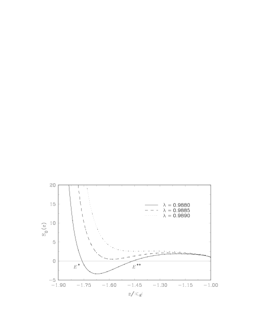
FIG. 2.: Graphs of the function ${\rm S}_{0}(z)$ at real $z\leq\epsilon_{d}$ for three values of $\lambda<1$ . The notations used: $E^{*}=E_{t}^{(2)*}/|\epsilon_{d}|$, $E^{**}=E_{t}^{(2)**}/|\epsilon_{d}|$.