Application of the time-dependent local-density approximation to conjugated molecules

Abstract

The time-dependent local-density approximation (TDLDA) is applied to the optical response of conjugated carbon molecules in the energy range of 0-30 eV, with calculations given for carbon chains, polyenes, retinal, benzene and C₆₀. The major feature of the spectra, the collective $\pi-\pi^{*}$ transition, is seen at energies ranging from below 2 to 7 eV, and is reproduced by the theory to a few tenths of an eV with a good account of systematic trends. However, there is some indication that TDLDA predicts too much fragmentation of the strength function in large molecules. Transition strengths are reproduced with a typical accuracy of 20%. The theory also predicts a broad absorption peak in the the range 15-25 eV, and this feature agrees with experiment in the one case where quantitative data is available (benzene).

I Introduction

Mean field theory is widely used in chemistry and physics, giving an approximation that is very robust in its domain of validity. Particularly successful is the density-functional theory[1], which treats the electron-electron interaction in a local-density approximation (LDA), i.e. by adding a density-dependent contact term to the Hartree Hamiltonian. This is similar to the $\alpha X$ approximation, but the contact term includes an approximate treatment of correlation effects as well as the exchange interaction. The theory is commonly used to calculate ground state structures of molecules and condensed systems. A corresponding theory for excitations is the time-dependent local-density approximation (TDLDA), which has also been applied to a number of systems [11, 2, 3, 4, 5, 6, 7, 8, 9, 10, 11, 12]. In this work, we will attempt to make a systematic survey of the predictions of the TDLDA for conjugated carbon molecules. Our calculations will be ab initio from the point of view of the electrons, since we take the electron Hamiltonian from well-known prescriptions used in ab initio density-functional Hamiltonians. However, we will not attempt to use the Hamiltonian to arrive at the nuclear coordinates; the ground state problem has been well studied by others and our interest here is in the excitations. In the next section we review the TDLDA theory and our numerical implementation of it. Then we discuss the predictions and comparison with experiment for carbon chains, polyenes, the aromatic ring, and C₆₀.

II Theory

A Formal aspects

The TDLDA theory is closely related to the time-dependent Hartree-Fock equation introduced by Dirac[13]. That theory can be derived from a variational principle,

$$\delta\int\,dt\,\langle\Psi|H-i\hbar{\partial\over\partial t}|\Psi\rangle=0.$$ (1)

Here $\Psi$ is restricted to be a Slater determinant of single-electron wave functions $\phi_{i}$, $\Psi={\cal A}\prod_{i}\phi_{i}$ . The corresponding static variational principle is the usual energy minimization principle from which one derives the Hartree-Fock equations. The LDA theory is obtained in the same way, using the LDA energy functional instead of $\langle\Psi|H|\Psi\rangle$ in eq. (1). The derived TDLDA equations of motion are given by

$$-{\hbar^{2}\nabla^{2}\over 2m}\phi_{i}+V_{ion}\phi_{i}+e^{2}\int\,dr^{\prime}{n(r^{\prime})\over|r-r|}\phi_{i}+V_{xc}[n(r)]\phi_{i}=i\hbar{\partial\over\partial t}\phi_{i}$$ (2)

where $n(r)=\sum_{i}|\phi_{i}(r)|^{2}$ is the electron density. The $V_{xc}$ is the exchange-correlation potential, related to the exchange-correlation energy $v_{xc}$ by $V_{ex}=dv_{xc}/dn$.

Several general remarks can be made here. Practitioners of the density-functional theory often claim justification for the Kohn-Sham equations based on formal existence theorems. Theorems can also be proven for the time-dependent case[14], but our own partiality to the theory is based on more pragmatic considerations. First, if the time dependence is slow, the TDLDA should be as good as the static theory because the motion would be adiabatic and governed by the same Hamiltonian. Second, integrals of the response over frequency obey sum rules, and these are satisfied in principle by the small-amplitude TDLDA. Since the sum rules are most sensitive to the high frequency behavior, we see that the TDLDA is good at both extremes, and therefore promising for describing the middle ground.

The next remark concerns the domain of applicability of the theory. The TDLDA describes the system by a single Slater determinant which can be expressed in a particle-hole basis as a particle-hole operator on the ground state. The theory thus does not contain the degrees of freedom necessary to describe excitations that have a more complex character than single-electron excitations. Not only will the experimental spectrum be more complex due to mixing of states of different particle-hole character but the coupling to vibrations will broaden the transitions on an energy resolution scale of a few tenths of an eV. However, even though the TDLDA only includes single-electron degrees of freedom, it is far superior to the static single-electron theory because it includes dynamic screening effects. The dynamic screening arises directly from the time dependence of the mean field potential. It shifts transition strength up out of the lowest particle-hole excitations into a higher frequency range, of course preserving the sum rule. This can be a very large effect; in the case of C₆₀ considered below the strength of the lowest excitations are reduced by an order of magnitude. In general, what we expect from the TDLDA is the frequency location and strengths of the strong transitions, but not details of its fragmentation into the eigenstates of the many-electron Hamiltonian.

There are several implementations of the TDLDA, particularly in the small-amplitude limit, which is all that concern us unless nonlinear optical properties are wanted. The real-time method has been applied in other fields to describe the small amplitude response[15, 16]. We emphasize that the time-dependent method we use here is equivalent to the response function method used in ref. [10, 9, 11] and the matrix RPA method used in ref. [6, 3, 17], provided only that the amplitude of the motion is small. Thus in principle the results depend only on the assumed energy density function, and not on the particular method used to solved the equations. Different methods are advantageous under different circumstances. The matrix RPA is the only one of these methods that can treat nonlocal interactions such as the Fock term. However, the matrix RPA method uses a particle-hole representation of the perturbed wave function, which becomes inefficient for systems having a large number of particles. The arguments comparing the numerical efficiency of different methods is given in ref. [8]. In brief, the basic object to be computed in the response function method is a $D\times D$ matrix, where $D$ is the dimensionality of the basis. In the time-dependent methods, the numerical object is the set of $N$ vectors of dimensionality $D$, where $N$ is the number of electrons. The computational effort scales with the size of the system as $ND$ for the time-dependent method with a sparse Hamiltonian, compared with $D^{3}$ for the inversion of the matrix in the response function methods.

B Numerical aspects

The important decisions in a numerical implementation of the TDLDA are the choice of basis, the choice of a local density function, and the choice of the basic quantity calculated: time-dependent wave function, energy eigenstates, or frequency response. We consider these aspects in turn.

1 Basis

The three most popular representations for the electron wave function are localized functions such as Gaussians or atomic orbitals (e.g., ref. [6]), planes waves, and more recently, spatial meshes[18]. We solve the TDLDA equations using a uniform spatial mesh, following closely the technique introduced in ref. [19]. An important advantage of spatial meshes is that the single-electron Hamiltonian is a sparse matrix. This allows one to consider vectors for the particle wave functions with many tens of thousands of points. Of course, a uniform spatial mesh has the disadvantage that the mesh size is determined by requirements of small regions next to the ion centers. This is alleviated somewhat by the use of pseudopotentials (see below). The important numerical parameters associated with the spatial mesh are the mesh spacing $\Delta x$ and the total number of mesh points $M$. Thus the molecules are calculated in a volume $V\sim M(\Delta x)^{3}$. The boundary condition at the surface of the volume is determined when the numerical representation of the differential operator in the Hamiltonian is constructed. For most of our calculations, the operator takes the wave function to be zero on the mesh points outside the volume. We use a higher-order difference operator in our program, as was done in ref. [19, 18]. The required mesh spacing depends on atoms involved; with carbon we use $\Delta x=0.3$ Å which gives a HOMO-LUMO gap to within 0.1 eV of the converged value for the Kohn-Sham equations. The geometry of the volume represented by the mesh is determined by requiring the edge to be at least 4 Å from any ionic center. The number of points needed ranges from 19000 in C₂H₄ to 103000 in C₂₈H₃₀.

2 Energy density function

For our energy density function, we use the widely applied exchange-correlation energy given by ref. [20, 21]. One can introduce more complicated energy functions that have gradient corrections or self-interaction corrections, but it was not clear that there would be an advantage in using a more complicated form.

In addition, we replace the ionic potential by a pseudopotential to eliminate the core electrons from the theory. In principle the theory should be used with all electrons, but in structure calculations the core electrons are passive and it is a computational waste to treat them explicitly. We use a standard prescription for constructing the pseudopotentials of the ions[22]. This procedure gives a pseudopotential that is nonlocal, depending on the orbital angular momentum of the electron. This has consequences for the sum rules[23], but we believe these are well under control[24]. Numerically, we implement the nonlocality using a separable approximation as described by ref.[25].

3 Ground state

The first part of the calculation is to construct the electronic ground state of the molecule with the same LDA Hamiltonian that will be used for the time-dependent calculation. We use an iterative conjugate-gradient method for this part of the calculation. Since the computation time taken just a small fraction of the total ($\sim 10\%$), it was not worthwhile to optimize this step[26]. It is very useful to compute at the same time the energies of occupied and unoccupied orbitals near the Fermi surface. Unlike the Hartree-Fock energies, the LDA single-particle energy differences provide a good approximation to particle-hole excitation energies in the molecules. The independent-particle model of the excitation spectrum is based on these energies and the matrix elements of the independent particle-hole states.

4 Time-dependent equations

Once one has the wave functions for the occupied ground state orbitals $\phi^{(0)}_{i}$, they are perturbed by multiplying them by a phase factor,

$$\phi_{i}(0)=e^{ikx}\phi^{(0)}_{i}.$$ (3)

Physically, this gives the effect of a short-duration electric field acting on the electrons. The wave functions are then evolved by the time-dependent equation of motion, eq. (2). Physical observables are extracted from the time-dependent wave function by Fourier transformation. A basic quantity to describe the molecule’s interactions is the dynamic polarizability $\alpha(\omega)$. This is essentially given by the Fourier transform of the time-dependent dipole moment:

$$\alpha(\omega)={e^{2}\over\hbar}\int\,dt\,e^{-i\omega t}\sum_{i}\langle\phi_{i}(t)|x|\phi_{i}(t)\rangle.$$ (4)

Another useful quantity is the strength function $S(\omega)$, whose integral is the total oscillator strength. This is defined

$$S(\omega)={2m\omega\over\pi\hbar^{2}k}\int\,dt\,\sin\omega t\sum_{i}\langle\phi_{i}(t)|x|\phi_{i}(t)\rangle.$$ (5)

We shall use the symbol $n_{e}$ (effective number of electrons) for integral of $S$ when we consider the excitation with a specific orientation of the electric field with respect to the molecule. The usual oscillator strength $f$ is the same quantity averaged over molecular orientations.

The numerical integration requires as a parameter the time step $\Delta T$ over which the single-particle Hamiltonian is treated as static. Within the time step the equations are solved by a predictor-corrector method as described in ref. [19]. The required size of the time step depends on the energy scale of the Hamiltonian. Thus one expects a dependence $\Delta T\sim(\Delta x)^{2}$. As a practical criterion, we determine $\Delta T$ by requiring the norm of the wave function to be accurately conserved. When that is the case, the energy is also conserved to good accuracy. We found that $\Delta T=0.001\hbar$/eV is needed for carbon structures with a mesh size of $\Delta x=0.3$ Å.

Another numerical parameter is the length of the time integration $T$. The effective resolution of the strength function is determined by this quantity. In the timing tests we show below, the integration time is $T=10~{}\hbar$/eV, corresponding to a resolution of $\hbar/T=0.1$ eV. In the graphs of the strength functions shown later we have integrated to $T=30-40~{}\hbar$/eV, giving peaks having widths of less than 0.1 eV. Since the accuracy of the TDLDA does not approach this value, there is no benefit to integrate to longer times. However, one must remember that the displayed strength functions have a spurious width due to the finite integration time. In principle, the TDLDA strength function is infinitely sharp below the ionization threshold.

As mentioned earlier, an advantage of the real-time implementation of the TDLDA is that the computing effort scales with the number of particles $N$ and the spatial dimension $D$ as $ND\sim N^{2}$. Methods using a particle-hole representation or the response scale as a higher power, at least if one applies the methods naively without truncation of matrix diagonalization or inversion operations. We have examined the scaling of our computation time for the polyenes, which discussed in detail in Sec. 4 below. The crosses in Fig. 1 show the computation time to set up the ground state wave function for series ethylene, butadiene, …,C₂₈H₃₀, using 1500 iterations of the Kohn-Sham equations. The abscissa gives the number of valence electrons in the calculation. The dashed line shows the dependence according to $t\sim N^{2}$ scaling. One sees that the $N^{2}$ scaling applies quite nicely to the larger sized molecules. The computation time for solving the time-dependent equation starting from the ground state is shown by the open triangles in Fig. 1. Here we used 10,000 time steps of 0.001 $\hbar$/eV to obtain the real-time response over an interval of 10 $\hbar$/eV. From the figure, we see that the scaling is even a little weaker than $N^{2}$. In fact the number of points $D$ needed to represent the wave function scales more slowly than $M\sim N$ due to surface effects.

III Carbon chains

The first carbon structures we applied the theory to are linear carbon chains. The results were already reported in [8], but for completeness we summarize them here. In that study we assumed that the chains were straight with evenly spaced carbon atoms. The interesting quantities are the HOMO-LUMO gap

$$\Delta e=e_{LUMO}-e_{HOMO}$$ (6)

and the behavior of the collective $\pi-\pi^{*}$ excitation. The HOMO-LUMO gap for molecules in the range C₃-C₂₀ is well described by the simple parameterization

$$\Delta e={A\over N+1}$$ (7)

with $A=17.5$ eV for even chains and $A=16$ eV for odd chains. This corresponds to the Hückel model with a hopping parameter $\beta=2.8$ eV. Experimentally, transitions have been observed at these energies for even-$N$ chains with $6\leq N\leq 12$.

The TDLDA predicted that the collective excitation was a single, sharp state with a energy that varies more slowly with $N$ than eq. (7). A better fit can be made with the following functional form[27]

$$E=A{\sqrt{lnN}\over N}.$$ (8)

The large-$N$ fit to eq. (8) has $A=31.7$ eV with no difference between odd and even $N$. Configuration-interaction quantum chemistry calculations have been done for $N=3,5$ and 7[28, 29], and the energies of the predicted collective excitations agree well with TDLDA. Experimentally, transitions have been observed for odd-$N$ molecules with $N=3,7,9,11,13$ and 15. The systematics follows eq. (8) with a coefficient that is 10% lower, $C\approx 28.3$.

The oscillator strength associated with the $\pi-\pi^{*}$ transition was found to be the same in the independent electron calculation as in the TDLDA. This implies that the screening due to the $\sigma$-electrons is weak. The longitudinal oscillator strength was found to depend on the number of atoms in the chain roughly as

$$n_{e}=C(N-1)$$ (9)

with $C\approx 1.6$. This oscillator strength has a physical interpretation as the number of electrons in the $\pi$ manifold of states. For odd-$N$ chains, that number is $2N-2$, about 20% larger than eq. (9).

IV Polyenes

We next consider the polyenes with alternating double and single bonds which have been studied in empirical models[30] and well as with the linear response[4, 5]. Unlike the small carbon chains, the polyene bonds lengths are not equal. As a consequence the HOMO-LUMO gap goes to a finite value rather than to zero as in eq. (7). Our structures have bond lengths of 1.45 Å for C-C bonds and 1.34 Å  for double C=C bonds, as is commonly assumed. The C=C-C and C=C-H bond angles are taken to be 124^∘ and 119^∘ respectively, in the all-trans conformation. We first discuss a typical case, C₈H₁₀. Fig. 2 shows on left the energies of the $\pi$ orbitals in the LDA calculation of the ground state. On the right-hand side is the spectrum of the Hückel model which will be discussed below. Both the HOMO and the LUMO are in the $\pi$ manifolds indicated in the Figure; the HOMO-LUMO energy gap is 2.58 eV in the LDA. The HOMO-LUMO transition has an oscillator strength of $n_{e}=5.3$ in the LDA. For comparison, the strength would be $n_{e}=8$ if that transition absorbed all of the strength of the $\pi$ manifold, since there are 8 electrons in the occupied $\pi$ orbitals. The 35% reduction from the nominal value is more severe than in the carbon chains; evidently the longer bond distances in the polyenes cause some fragmentation of the strength.

Next we show in Fig. 3 the TDLDA response of C₈H₁₀ from zero energy to 30 eV excitation. One sees the strong $\pi-\pi^{*}$ transition at 3.86 eV, with a strength $n_{e}=3.9$. The slight reduction of strength compared to the single-electron picture is due to the screening effect of the $\sigma$ electrons. In Fig. 3 one also sees the $\sigma-\sigma^{*}$  transitions as the broad distribution between 10 and 20 eV. The strength integrated up to 30 eV is $n_{e}=30$; integrating up to 100 eV gives a strength of 41 which compares well to the number of valence electron in C₈H₁₀, namely 42.

We next turn to the systematics as a function of the length of the polyene molecule. Fig. 4 shows the HOMO-LUMO gap and the excitation energy of the strong $\pi-\pi^{*}$ transition as a function of the number of carbon atoms. The HOMO-LUMO gap systematics is compared to two functional forms in the figure. The dot-dash line shows an $N^{-1}$ dependence as in eq. (7), which is clearly wrong. The dashed line is a fit to the generalized Hückel model with two hopping parameters $\beta_{s}$ and $\beta_{d}$ corresponding to the single and double CC bonds, respectively. For the fit, the parameter values are

$$\beta_{s}=-2.27{\rm~{}eV~{}and}~{}~{}\beta_{d}=-2.80~{}{\rm eV.}$$ (10)

These are somewhat larger than the values assumed in ref. [30]. The fit for the finite systems is quite good, showing that rather simple considerations are sufficient to describe the Kohn-Sham single particle energies. Our fit parameters would give a band gap of 0.86 eV in infinitely long polyene molecules.

The collective transition in the TDLDA has more complex behavior for large polyenes. We find, unlike the carbon chains, that the $\pi-\pi^{*}$ strength is partly split in the larger polyenes. This is shown in Fig. 5, showing the low-energy TDLDA strength function for N=8,18, and 28. The systematics of the energy of the strongest states is also shown in Fig. 4 as the crosses. We have not found a theoretically motivated analytic parametrization for the $n$-dependence of these transitions. The PPP empirical theory [30], when fitted to the smaller polyenes, gives too high an energy for the largest ones, as is shown by the dotted line in Fig. 4. In Fig. 6 we show the comparison with experiment and with the linear response calculations of ref. [4, 5]. The two calculations agree well with each other for the lighter systems, but they severely diverge for the heavier molecules. In principle, the small-amplitude TDLDA and the linear response are just different mathematical formulations of the same theory, and they should give the same results for the same Kohn-Sham energy functional. Perhaps the differences are due to different assumed bond lengths, as mentioned in the footnote. The experimental data for polyenes in solution is shown by the crosses and squares. There is also gas phase data quoted in ref. [5] which gives 10% higher energies. From Fig. 6 one sees good agreement with the lighter polyenes, but the data falling between the two theoretical calculations for the heavier ones.

The predicted transition strengths for the two calculations are also significantly different. Fig. 7 shows the oscillator strengths in our calculation, compared to the nominal strength in the $\pi$ manifold. The HOMO-LUMO transition, shown by the triangles, has roughly half the nominal strength. This is further decreased in the TDLDA by two effects. One is the screening by the $\sigma$ electrons, and the other is the loss of strength in the heavier polyenes to other states. In contrast, the calculation of [5] gave a collective transition with about 75% of the nominal strength for the heavier polyenes. The stronger collectivity then gives a larger upper shift in the energy from the HOMO-LUMO gap position.

As a final example closely related to the polyenes, we examine retinal, the molecule of biological prominence as a retinyl chromophore. Retinal is more complicated than a polyene, having an aromatic termination on one end and an carboxyl group on the other, but these play a minor role in the collective longitudinal excitation. We consider the all-trans form, which is the final state of the chromophore having absorbed a photon. The experimental data[33] on all-trans-retinal shows broad, asymmetric peak with a maximum at 3.2 eV and a full width at half maximum of about 0.6 eV. There is a previous ab initio study using the CASSCF method[34] which we can also compare to. In our calculation, the HOMO-LUMO gap is 2.0 eV, and this state is very strong in the single-electron approximation. The electron-electron interaction in the TDLDA shifts the center of gravity of the strength up to 3.3 eV, close to the experimentally observed position. In contrast, the calculation of ref. [34] obtained the strong transition at much higher energy. However, as may be seen from Fig. 8, the TDLDA strength is fragmented into three states. The LDA predicts the existence of a number of particle-hole states in the 3 eV energy region, and the residual electron interaction is strong enough to mix them. The lowest predicted strong state, at 2.5 eV, is in a spectral region where the empirical absorption strength is small. This is similar to the problem we had with the large polyenes. In the retinal case, however, the situation is complicated by the presence of an oxygen atom on the molecule. As discussed in ref. [34], the lowest excitation in the molecule has a predominant component with a hole at the oxygen. We have not checked that our mesh size $\Delta x=0.3$ Å is small enough to describe oxygen reliably, and that needs to be checked before making a final conclusion on the accuracy of the TDLDA for this system. The transition strength associated with the three strong transitions is $f=1.7$ in the TDLDA, which is close to the prediction of ref. [34], but twice our extracted experimental value. That was obtained using the extinction coefficient data of ref. [33], correcting the solution data by the Debye factor[35].

V Simple aromatic molecules

We discuss here the optical absorption spectra of benzene and C₆₀.

A Benzene

Benzene provides our best example of the TDLDA comparisons to experiment. For this calculation, we take the empirical geometry of benzene, $D_{6}$ symmetry with CC bond length of 1.396 Å and CH bond length of 1.083 Å. The static LDA calculation gives an energy spectrum with a gap $\Delta e$ of 5.04 eV. This may be compared with the empirical energy of the ${}^{1}B_{2u}$ excitation, which is a $\pi-\pi^{*}$  particle-hole state having a small residual interaction. That energy is 4.9 eV[36], close to the LDA prediction. Other recent calculations of benzene excitations have been made using the CASSFC and MRMP methods[37]. These authors find that the ${}^{1}B_{2u}$ is also well reproduced by the CASSFC but not so well by the MRMP.

Turning to the dynamic response, the TDLDA transition strength is shown in Fig. 10. One sees the collective $\pi-\pi^{*}$ state as a narrow peak at 6.9 eV. Thus the residual interaction pushes the $\pi-\pi^{*}$ strength up 1.9 eV from its original position at $\Delta e$. Above 9 eV there is a broad feature peaking around 18 eV. This is associated with the $\sigma-\sigma^{*}$ transitions; the width is due to the high level density of particle-hole states in the region of the resonance, and the fact that they are unbound. However, our implementation of TDLDA uses a finite sized box, which does not give a satisfactory treatment of continuum effects. This spectrum was calculated putting an absorptive boundary condition on the wave function at the edge of the box. Instead of the very fine structure predicted with a reflecting boundary condition, the absorptive evidence produces (spurious) broader structures.

To compare with the empirical strength function, we consider data reported in two experiments. In ref. [36], the absolute strength was measured for excitation energies up to about 10 eV. There is a quite sharp state at 6.9 eV in very good agreement with our predicted $\pi-\pi^{*}$ transition. Comparing with the other theoretical methods, the strong state is well reproduced by the the MRMP but not the CASSCF[37]. The empirical strength integrating the peak region from 6.5 eV up to the minimum at 8.3 eV is $f=0.9$ eV. This agrees well with our theoretical strength for the collective transition, $f=1.1$. Here both the CASSCF and MRMP give even better agreement with experiment. We mention that none of the theories describe the finer details of the absorption spectrum around the 6.9 eV peak, which has an asymmetric tail and a small peak on the low-energy side. Since theory predicts a single sharp state, it is clear that other degrees of freedom, probably the vibrational, are responsible for the detailed structure of the peak. The experimental strength function also show very fine peaks in the neighborhood of the ionization energy. These are Rydberg states which are beyond the reach of simple energy densities functions, which lack the Coulomb tail in the mean field. Another experiment[38] reported the absorption strength going up to much higher energies, but without an absolute normalization. In Fig. 10 we show this data normalized to our calculation. We see that broad $\sigma-\sigma^{*}$ feature is reproduced in position and width very well. However as mentioner, fine details of the spectrum are not properly reproduced.

VI C₆₀

Our last example is the molecule C₆₀. This molecule has been well studied in the LDA; the predicted HOMO-LUMO gap is 1.65 eV, compared with the measured gap of $\sim 1.6$ eV. The strength function computed with the TDLDA is shown in Fig. 11. We see a set of strong transitions in the region 4-7 eV excitation, and a much larger and broad set in the region of 15-30 eV. The lower transitions have a $\pi-\pi^{*}$character. Experimentally, the absorption strength below 6 eV has been measured in absolute terms and the data is reviewed in ref. [39]. Comparison of theory and experiment is made in Table I. There is a good correspondence between the TDLDA transition at 3.4 eV and the observed state at 3.8 eV. For the higher transitions, theory predicts more strong states than the number of peaks observed, so there is no one-to-one correspondence. However, the overall strength distribution comes out fairly well. This may be seen in Fig. 12 comparing the integrated strength distribution up to 6.2 eV. Of course the TDLDA strength is sharply peaked without the line-broadening processes that would be computable in a more complete theory. The total strength in the region comes out about right in TDLDA, but shifts of the order of 0.5 eV would be required to fit the data.

The strong absorption between 15 and 30 eV is due to $\sigma-\sigma^{*}$ transitions. Of course, the sharp structures predicted in the TDLDA would be smeared out due to coupling to the continuum and to vibrations. The only data in this region is the photoelectron cross sections[40]. It shows a peak at 20 eV having a full width at half maximum of about 10 eV, consistent with the TDLDA results.

VII Conclusion

The TDLDA is an attractive theory for collective excitations in large molecules because of its numerical scaling properties, and its automatic compliance with sum rules. We have found it to be rather good for conjugated carbon molecules, giving a reasonable account of the strong transitions in both the $\pi-\pi^{*}$  and $\sigma-\sigma^{*}$ manifolds of states.

In the $\pi-\pi^{*}$ manifold, the energetics of the underlying single-particle states are fairly well described by the Hückel Hamiltonian. The results are summarized in Fig. 13, showing the deduced hopping matrix elements as a function of the CC bond length. Fitting the conjugated molecules to a power law dependence on bond length, the extracted matrix elements vary as $t\sim r^{-2.7}$. This is a stronger dependence than the commonly assumed form, $t\sim r^{-2}$. The matrix element for the carbon chain molecules is quite different, perhaps because of the absence of hydrogen atoms.

As is well known, the electron-electron interaction strongly perturbs the absorption strength function. In the region of the $\pi-\pi^{*}$ transitions, the strength is shifted upward by an amount of the order of 1-2 eV for the systems studied. In the case of carbon chains, the transition energy can be described fairly well analytically. The energies agree well with the empirical values for the smaller molecules, but the larger ones are predicted to have more fragmentation of strength in the TDLDA than is observed. The amount of strength in the $\pi-\pi^{*}$ transition in principle depends on the coupling to the other electrons. In small or extended molecules, the coupling and resulting screening is rather mild, less than a factor of two. On the other hand, in C₆₀ the $\pi-\pi^{*}$ transition strength is more strongly screened. The absorption spectra typically have a gap above the the strong $\pi-\pi^{*}$ transition, followed by a dense spectrum of $\sigma-\sigma^{*}$ transitions above 10 eV. This spectrum peaks in the range of 15-20 eV and is quite broad. This feature is present in the empirical absorption, but quantitative experimental data is only available for one case, benzene. There we found good agreement on the overall shape and size of the $\sigma-\sigma^{*}$ absorption peak. In view of the evident success of the TDLDA theory, it would be interesting to consider more ambitious applications. One direction is to try other, more difficult, elements. In particular, it may be possible to treat $d$-shell elements with mesh sizes of the order of $\Delta x\approx 0.2$ Å, which would allow small molecules and clusters to be calculated. Another direction would be to study the effect of perturbations on the spectra. Possible perturbations include: nearby charges or nearby molecules; thermal distributions of ionic geometries; electron-vibration coupling.

This work is supported in part by the Department of Energy under Grant DE-FG-06-90ER40561, and by the Grant-in-Aid for Scientific Research from the Ministry of Education, Science and Culture (Japan), No. 09740236. Numerical calculations were performed on the FACOM VPP-500 supercomputer in the institute for Solid State Physics, University of Tokyo, and on the NEC sx4 supercomputer in the research center for nuclear physics (RCNP), Osaka University.

TABLE I.: Oscillator strengths $f$ for the near-ultraviolet transitions in C₆₀

TDLDA	TDLDA	experiment	experiment
E (eV)	$f$	E (eV)	$f$
3.4	0.3	3.8	0.5
4.3	0.9
5.3	2.5	4.8	2.1-2.5
6.0	2.5	5.8	5-6
6.6	1.1

Figure Captions

Fig. 1 Computation times for the TDLDA method. Shown are the times in minutes for computation of polyenes on the NEC sx4 vector process computer, with an effective speed of 0.4 Gflop, as a function of the number of of electrons in the molecule. Crosses show the time to construct the ground state, taking 1500 iteration steps. Open triangles show the duration of the time-evolution phase of the calculation, taking 10000 iteration steps.A quadratic functional dependence is displayed with the lines.

Fig. 2 C₈H₁₀ orbitals with $\pi$ character. The left-hand side shows the results of the static LDA calculation. The spectrum of the Hückel Hamiltonian with matrix elements given by eq. (10) is shown on the right. The energies of the Hückel spectrum have been shifted to match the position of the HOMO state.

Fig. 3 Strength function of C₈H₁₀ in the energy region 0-30 eV, calculated in the TDLDA.

Fig. 4 Results of the present TDLDA calculations for polyenes, C_nH_n+2. The HOMO-LUMO gap is shown by the triangles, and the fit to the generalized Hückel Hamiltonian with matrix elements eq. (10) by the dashed line. For comparison, the $n^{-1}$ dependence similar to eq. (7) is shown by a dot-dashed line. The energies of the strongest transition in TDLDA are shown by crosses. The strong transition in the PPP empirical theory is shown by the dotted line.

Fig. 5 TDLDA strength function for low-energy transitions in the polyenes with $n=8,18$ and 28.

Fig. 6 Energy of the collective $\pi-\pi^{*}$ transition in polyenes, comparing theory with experiment. The solid line connects the energies found from the TDLDA, and the dashed line connects the results of [5]. Crosses and squares are data in solution from ref. [32] and [31], and triangles are gas data as quoted by ref. [5].

Fig. 7 Strengths of the collective $\pi-\pi^{*}$ transitions in polyenes: single-electron HOMO-LUMO transition, triangles; collective TDLDA transition, crosses. The total strength associated with the $\pi$ manifold is shown by the dashed line.

Fig. 8 Strength function for retinal; TDLDA, solid; experiment [33], dashed.

Fig. 9 Benzene orbital energies in the static LDA. On the far right are the $\pi$ energies in the Hückel model, with $\beta=2.52$ eV, shifted to match the HOMO energy.

Fig. 10 Optical absorption of the benzene molecule, in units of eV^-1. a) experimental, from ref. [38]; b) TDLDA. An absorptive potential has been put at the boundaries of the grid to mimic the continuum. The grid has the shape of a sphere of radius 7 Å with $\Delta x=0.3$ Å and $\Delta t=0.001$ eV^-1. The number of spatial mesh points is about 50,000. The figure shows the Fourier tranform of real-time response over a time $T=30$ eV^-1.

Fig. 11. Strength for C₆₀ calculated in the TDLDA.

Fig. 12. Integrated strength below 6.2 eV in C₆₀, TDLDA, dashed line; experiment [39], solid line.

Fig. 13. Effective Hückel matrix elements in the molecules studied. They are, in ordering of increasing bond length: carbon chains,polyene single bond, benzene, and polyene double bond.

FIG. 1.: Computation times for the TDLDA method. Shown are the times in minutes for computation of polyenes on the NEC sx4 vector process computer, with an effective speed of 0.4 Gflop, as a function of the number of of electrons in the molecule. Crosses show the time to construct the ground state, taking 1500 iteration steps. Open triangles show the duration of the time-evolution phase of the calculation, taking 10000 iteration steps.A quadratic functional dependence is displayed with the lines.

FIG. 2.: C₈H₁₀ orbitals with $\pi$ character. The left-hand side shows the results of the static LDA calculation. The spectrum of the Hückel Hamiltonian with matrix elements given by eq. (10) is shown on the right. The energies of the Hückel spectrum have been shifted to match the position of the HOMO state.

FIG. 3.: Strength function of C₈H₁₀ in the energy region 0-30 eV, calculated in the TDLDA.

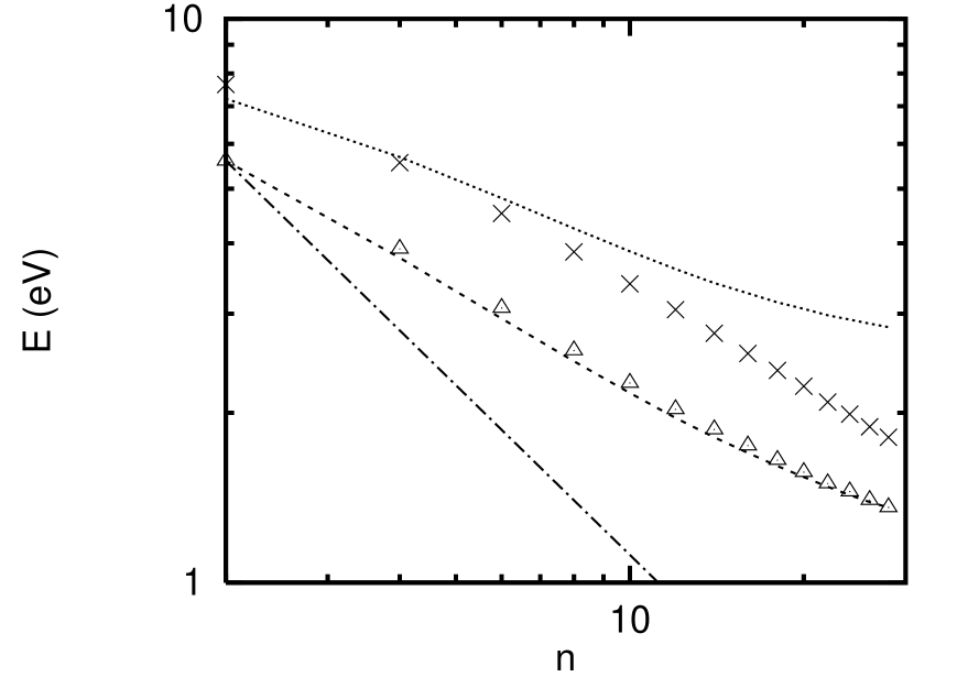
FIG. 4.: Results of the present TDLDA calculations for polyenes, C_nH_n+2. The HOMO-LUMO gap is shown by the triangles, and the fit to the generalized Hückel Hamiltonian with matrix elements eq. (10) by the dashed line. For comparison, the $n^{-1}$ dependence similar to eq. (7) is shown by a dot-dashed line. The energies of the strongest transition in TDLDA are shown by crosses. The strong transition in the PPP empirical theory is shown by the dotted line.

FIG. 5.: TDLDA strength function for low-energy transitions in the polyenes with $n=8,18$ and 28.

FIG. 6.: Energy of the collective $\pi-\pi^{*}$ transition in polyenes, comparing theory with experiment. The solid line connects the energies found from the TDLDA, and the dashed line connects the results of [5]. Crosses and squares are data in solution from ref. [32] and [31], and triangles are gas data as quoted by ref. [5].

FIG. 7.: Strengths of the collective $\pi-\pi^{*}$ transitions in polyenes: single-electron HOMO-LUMO transition, triangles; collective TDLDA transition, crosses. The total strength associated with the $\pi$ manifold is shown by the dashed line.

FIG. 8.: Strength function for retinal; TDLDA, solid; experiment [33], dashed.

FIG. 9.: Benzene orbital energies in the static LDA. On the far right are the $\pi$ energies in the Hückel model, with $\beta=2.52$ eV, shifted to match the HOMO energy.

FIG. 10.: Optical absorption of the benzene molecule, in units of eV^-1. a) experimental, from ref. [38]; b) TDLDA. An absorptive potential has been put at the boundaries of the grid to mimic the continuum. The grid has the shape of a sphere of radius 7 Å with $\Delta x=0.3$ Å and $\Delta t=0.001$ eV^-1. The number of spatial mesh points is about 50,000. The figure shows the Fourier tranform of real-time response over a time $T=30$ eV^-1.

FIG. 11.: Strength for C₆₀ calculated in the TDLDA.

FIG. 12.: Integrated strength below 6.2 eV in C₆₀, TDLDA, dashed line; experiment [39], solid line.

FIG. 13.: Effective Hückel matrix elements in the molecules studied. They are, in ordering of increasing bond length: carbon chains,polyene single bond, benzene, and polyene double bond.

REFERENCES

- [1] R.O. Jones, O. Gunnarsson, Rev. Mod. Phys. 61 689 (1989).
- [2] C. Yannouleas, et al., J. Phys. B27 L642 (1994).
- [3] H. Koch, et al., Chem. Phys. 172 13 (1993).
- [4] Y. Luo, et al., J. Phys. Chem. 98 7782 (1994).
- [5] Y. Luo, et al., Phys. Rev. B51 14949 (1995).
- [6] M. Feyereisen, et al., J. Chem. Phys. 96 2978 (1992).
- [7] K. Yabana and G.F. Bertsch, Phys. Rev. B54 4484 (1996).
- [8] K. Yabana and G.F. Bertsch, Z. Phys. D42 219 (1997).
- [9] C. Jamorski, et al, J. Chem. Phys. 104 5134 (1996).
- [10] X. Blase, et al., Phys. Rev. B52 R2225 (1995).
- [11] A. Rubio, et al., Phys. Rev. Lett. 77 247 (1996).
- [12] A. Zangwill and P. Soven, Phys. Rev. A21 (1980) 1561.
- [13] P.A.M. Dirac, Proc. Cambridge Phil. Soc. 26 376 (1930).
- [14] M. Petersilka, U. Grossmann, and E. Gross, Phys. Rev. Lett. 76 1212 (1996).
- [15] F.V. DeBlasio, et al., Phys. Rev. Lett. 68 1663 (1992).
- [16] D. Vretanar, et al., Nucl. Phys. A621 853 (1997).
- [17] C. Yannouleas, et al., Phys. Rev. B47 9849 (1993); F. Alasia, et al., J. Phys. B27 L643 (1994).
- [18] J. Chelikowsky, N. Troullier, K. Wu, and Y. Saad, Phys. Rev. B50 11355 (1994).
- [19] H. Flocard, S. Koonin, and M. Weiss, Phys. Rev. C17 1682 (1978).
- [20] D. Ceperley and B. Alder, Phys. Rev. Lett. 45 566 (1980).
- [21] J. Perdew and A. Zunger, Phys. Rev. B23 5048 (1981).
- [22] N. Troullier, J.L. Martins, Phys. Rev. B43 1993 (1991).
- [23] P. Alippi, P. La Rocca, and G. Bachelet, Phys. Rev. B55 13855 (1997).
- [24] K. Yabana and G.F. Bertsch, to be published in Phys. Rev. A; Los Alamos preprint phys/9802017.
- [25] L. Kleinman and D. Bylander, Phys. Rev. Lett. 1425 (1982).
- [26] Y. Saad, et al., BIT 36 563 (1996).
- [27] Y. Mizuno and T. Izuyama, Prog. Theo. Phys. 21 593 (1959).
- [28] G. Paacchioni and J. Koutecky, J. Chem. Phys. 88 1066 (1988).
- [29] M. Kolbuszewski, J. Chem. Phys. 102 3679 (1995).
- [30] K. Schulten, I. Ohmire, and M. Karplus, J. Chem. Phys. 64 4422 (1976).
- [31] F. Sondheimer, et al., J. Am. Chem. Soc. 83 1675 (1961).
- [32] M.F. Granville, et al., J. Chem. Phys. 75 3765 (1981).
- [33] R.R. Birge, et al., J. Am. Chem. Soc. 104 1196 (1982).
- [34] M. Merchan and R. Gonzales-Luque, J. Chem. Phys. 106 1112 (1997).
- [35] P. Debye, Polar Molecules (Chemical Catalog, New York, 1929).
- [36] A. Hiraya and K. Shobatake, J. Chem. Phys. 94 (1991) 7700.
- [37] T. Hashimoto, H. Nakano, and K. Hirano, J. Chem. Phys. 104 6244 (1996).
- [38] E.E. Koch and A. Otto, Chem. Phys. Lett. 12 (1972) 476.
- [39] A.L. Smith, J. Phys. B29 4975 (1996).
- [40] I.V. Hertel et al., Phys. Rev. Lett. 68 784 (1992).