1D Toy Model For Trapping Neutral Particles

Abstract

We study, both classically and quantum-mechanically, the problem of a neutral particle with a spin $S$, mass $m$ and magnetic moment $\mu$, moving in one dimension in an inhomogeneous magnetic field given by

$$\mathbf{B}=B_{0}\mathbf{\hat{z}+}B_{\bot}^{\prime}x\mathbf{\hat{y}.}$$

This problem serves for us as a toy model to study the trapping of neutral particles. We identify

$$K\equiv\sqrt{\dfrac{S^{2}\left(B_{\bot}^{\prime}\right)^{2}}{\mu mB_{0}^{3}}},$$

which is the ratio between the precessional frequency of the particle and its vibration frequency, as the relevant parameter of the problem.

Classically, we find that when $\mu$ is antiparallel to $\mathbf{B}$, the particle is trapped provided that $K<0.5$. We also find that viscous friction, be it translational or precessional, destabilizes the system.

Quantum-mechanically, we study the problem of a spin $S=\hbar/2$ particle in the same field. Treating $K$ as a small parameter for the perturbation from the adiabatic Hamiltonian, we find that the lifetime $T_{esc}$ of the particle in its trapped ground-state is

$$T_{esc}=T_{vib}\sqrt{\dfrac{1}{\left(2\pi\right)^{3}K}}\exp\left[\dfrac{1}{2K}\right]\text{ ,}$$

where $T_{vib}=2\pi\sqrt{mB_{0}/\mu\left(B_{\bot}^{\prime}\right)^{2}}$ is the classical period of the particle when placed in the adiabatic potential $V=\mu\left|\mathbf{B}\right|$.

1 Introduction.

1.1 Magnetic traps for neutral particles.

Recently there has been rapid progress in techniques for trapping samples of neutral atoms at elevated densities and extremely low temperatures. The development of magnetic and optical traps for atoms has proceeded in parallel in recent years. While optical methods have proved to be an efficient means of cooling atoms to temperatures in the microKelvin range, further progress is limited by interatomic interactions induced by the scattering of photons. The effort to attain higher densities and lower temperatures has therefore concentrated on the development of purely magnetic traps[1, 2, 3, 4, 5, 6, 7]. Such traps exploit the interaction of the magnetic moment of the atom with the inhomogeneous magnetic field to provide spatial confinement.

Microscopic particles are not the only candidates for magnetic traps. In fact, a vivid demonstration of trapping large-scale objects is the hovering magnetic top[8, 9, 10]. This ingenious magnetic device, which hovers in mid-air for about 2 minutes, has been studied recently by several authors [11, 12, 13, 14].

1.2 Qualitative description.

The physical mechanism underlying the operation of magnetic traps is the adiabatic principle. The common way to describe their operation is in terms of classical mechanics: As the particle is released into the trap, its magnetic moment points antiparallel to the direction of the magnetic field. While inside the trap, the particle experiences lateral oscillations $\omega_{vib}$ which are slow compared to its precession $\omega_{prec}$. Under this condition the spin of the particle may be considered as experiencing a slowly rotating magnetic field. Thus, the spin precesses around the local direction of the magnetic field $\mathbf{B}$ (adiabatic approximation) and, on the average, its magnetic moment $\mathbf{\mu}$ points antiparallel to the local magnetic field lines. Hence, the magnetic energy, which is normally given by $-\mathbf{\mu}\cdot\mathbf{B}$, is now given (for small precession angle) by $\mu\left|\mathbf{B}\right|$. Thus, the overall effective potential seen by the particle is

$$V_{eff}\simeq\mu\left|\mathbf{B}\right|.$$ (1)

In the adiabatic approximation, the spin degree of freedom is rigidly coupled to the translational degrees of freedom, and is already incorporated in Eq.(1). Thus, under the adiabatic approximation, the particle may be considered as having only translational degrees of freedom. When the strength of the magnetic field possesses a minimum, the effective potential becomes attractive near that minimum and the whole apparatus acts as a trap. To prevent spin-flip (Majorana transitions), most magneto-static traps include a bias field, so that the effective potential $V_{eff}$ possesses a nonvanishing minimum.

As mentioned above, the adiabatic approximation holds whenever $\omega_{prec}\gg\omega_{vib}$. As $\omega_{prec}$ is inversely proportional to the spin, this inequality can be satisfied provided that the spin of the particle is small enough. If, on the other hand, the spin of the particle is too large, it cannot respond fast enough to the changes of the direction of the magnetic field. In this limit $\omega_{prec}\gg\omega_{vib}$, the spin has to be considered as fixed in space and, according to Earnshaw’s theorem[15], becomes unstable against translations.

1.3 The purpose and structure of this paper.

The discussion of magnetic traps in the literature is, almost entirely, done in terms of classical mechanics. In microscopic systems, however, quantum effects become dominant, and in these cases quantum mechanics is suited for the description of the trap. An even more interesting issue is the understanding of how the classical and quantum descriptions of a given system are related. In this paper we study, both classically and quantum-mechanically, the quantitative nature of magnetic traps. In order to keep the underlying physics transparent, we devise a simplified model for the inhomogeneous magnetic field of such traps. We further neglect the effect of interactions between the particles in the trap and so we analyze the dynamics of a single particle inside the trap. For simplicity, the particle is considered to have only a single translational degree of freedom. Its spin degree of freedom, on the other hand, is taken completely into account.

The structure of this paper is as follows: In Sec.2 we start by defining the system we study, together with useful parameters that will be used throughout this paper. Next, we carry out a classical analysis of the problem in Sec.3. Here, we find two stationary solutions for the particle inside the trap. One of them corresponds to a state whose spin is parallel to the direction of the magnetic field whereas the other one corresponds to a state whose spin is antiparallel to that direction. When considering the dynamical stability of these solutions, we find that only the antiparallel stationary solution is stable. We also study the same problem but with viscous friction added, and arrive at the interesting result that friction destabilizes the system. In Sec.4 we reconsider the problem, from a quantum-mechanical point of view. Here, we also find states that refer to parallel and antiparallel orientations of the spin, one of them being bound while the other one unbounded. In this case, however, these two states are coupled due to the inhomogeneity of the field, and we move on to calculate the lifetime of the bound state. Finally, in Sec.5 we compare the results of the classical analysis with those of the quantum analysis and comment on their implications for practical magnetic traps.

2 Description of the problem.

We consider a particle of mass $m$, magnetic moment $\mu$ and intrinsic spin $S$ (aligned with $\mu$) moving in 1D space in an inhomogeneous magnetic field $\mathbf{B}$ given by

$$\mathbf{B=}B_{0}\mathbf{\hat{z}+}B_{\bot}^{\prime}x\mathbf{\hat{y}}\text{.}$$ (2)

This field possesses a nonzero minimum of amplitude at the origin, which is the essential part of the trap. Note also that the direction of the field twists ( or curls) as one moves along the $x$ axis. The Hamiltonian for this system is

$$H=\dfrac{P^{2}}{2m}-\mathbf{\mu\cdot B}$$ (3)

where $P$ is the momentum of the particle.

We define $\omega_{prec}$ as the precessional frequency of the particle when it is at the origin $x=0$. Since at that point the magnetic field is $\mathbf{B=}B_{0}\mathbf{\hat{z}}$ we find that

$$\omega_{prec}\equiv\dfrac{\mu B_{0}}{S}\text{.}$$ (4)

Next, we define $\omega_{vib}$ as the small-amplitude vibrational frequency of the particle when it is placed in the adiabatic potential field given by

$$V(x)=\mu\left|\mathbf{B}(x)\right|=\mu B_{0}\left(1+\dfrac{1}{2}\left(\dfrac{B_{\bot}^{\prime}}{B_{0}}\right)^{2}x^{2}\right)+\mathcal{O}\left(x^{4}\right).$$

For this potential we have

$$k=\left.\dfrac{\partial^{2}V}{\partial x^{2}}\right|_{x=0}=\mu\dfrac{\left(B_{\bot}^{\prime}\right)^{2}}{B_{0}}\text{,}$$

and therefore

$$\omega_{vib}\equiv\sqrt{\dfrac{k}{m}}=\sqrt{\dfrac{\left(B_{\bot}^{\prime}\right)^{2}\mu}{mB_{0}}}\text{.}$$ (5)

We also define the ratio between $\omega_{vib}$ and $\omega_{prec}$,

$$K\equiv\dfrac{\omega_{vib}}{\omega_{prec}}=\sqrt{\dfrac{S^{2}(B_{\bot}^{\prime})^{2}}{\mu mB_{0}^{3}}}\text{.}$$ (6)

This will be our ‘measure of adiabaticity’. It is clear that as $K$ becomes smaller and smaller, the adiabatic approximation becomes more and more accurate. Note also that $K$ is the only possibility to form a non-dimensional quantity (up to an arbitrary power) out of the parameters of the system. The value of $K$ therefore, completely determines the behavior of the system.

3 Classical analysis.

3.1 The stationary solutions.

We denote by $\mathbf{\hat{n}}$ a unit vector in the direction of the spin (and the magnetic moment). Thus, the equation of motion for the center of mass of the particle is

$$m\dfrac{d^{2}x}{dt^{2}}=\mu\dfrac{\partial}{\partial x}\left(\mathbf{\hat{n}\cdot B}\right)\text{,}$$ (7)

and the evolution of its spin is determined by

$$S\dfrac{d\mathbf{\hat{n}}}{dt}=\mu\mathbf{\hat{n}\times B}\text{.}$$ (8)

The two equilibrium solutions to Eqs.(7) and (8) are

$$\mathbf{\hat{n}}(t) =\mp\mathbf{\hat{z}}$$ (9)

$$x(t) =0\text{,}$$

representing a motionless particle at the origin with its magnetic moment (and spin) pointing antiparallel ($\mathbf{\hat{n}}(t)=-\mathbf{\hat{z}}$) to the direction of the field at that point and a similar solution but with the magnetic moment pointing parallel to the direction of the field ($\mathbf{\hat{n}}(t)=+\mathbf{\hat{z}}$).

3.2 Stability of the solutions.

To check the stability of these solutions we now add first-order perturbations. We set

$$\mathbf{\hat{n}(}t\mathbf{)} =\mathbf{\mp\hat{z}+}\epsilon_{x}(t)\mathbf{\hat{x}+}\epsilon_{y}(t)\mathbf{\hat{y}}$$ (10)

$$x(t) =0+\delta x(t)\text{,}$$

substitute these into Eqs.(7) and (8), and retain only first-order terms. We find that the resulting equations for $\delta x(t)$, $\epsilon_{x}(t)$ and $\epsilon_{y}(t)$ are

$$\dfrac{d^{2}\delta x}{dt^{2}} =\dfrac{\mu B_{\bot}^{\prime}}{m}\epsilon_{y}$$ (11)

$$\dfrac{d\epsilon_{x}}{dt} =\dfrac{\mu}{S}\left(\epsilon_{y}B_{0}\pm B_{\bot}^{\prime}\delta x\right)$$

$$\dfrac{d\epsilon_{y}}{dt} =\mathbf{-}\dfrac{\mu}{S}\epsilon_{x}B_{0}\text{.}$$

We now look for oscillatory (stable) solutions for these equations. Setting

$$\delta x =x_{0}e^{-i\omega t}$$

$$\epsilon_{x} =\epsilon_{x,0}e^{-i\omega t}$$

$$\epsilon_{y} =\epsilon_{y,0}e^{-i\omega t}$$

inside Eqs.(11) yields

$$\underset{\mathbf{A}}{\underbrace{\left(\begin{array}[c]{lll}\omega^{2}&0&\mu B_{\bot}^{\prime}/m\\ \pm\mu B_{\bot}^{\prime}/S&i\omega&\mu B_{0}/S\\ 0&-\mu B_{0}/S&i\omega\end{array}\right)}}\cdot\left(\begin{array}[c]{l}x_{0}\\ \epsilon_{x,0}\\ \epsilon_{y,0}\end{array}\right)=\left(\begin{array}[c]{l}0\\ 0\\ 0\end{array}\right)\text{.}$$ (12)

This equation has non-trivial solutions whenever the determinant of the matrix $\mathbf{A}$ vanishes. Thus, the secular equation

$$\dfrac{K^{2}}{\omega_{vib}^{4}}\det\mathbf{A=}-K^{2}\left(\dfrac{\omega}{\omega_{vib}}\right)^{4}+\left(\dfrac{\omega}{\omega_{vib}}\right)^{2}\mp 1=0$$ (13)

determines the eigenfrequencies $\omega$ of the various possible modes. When the lower sign is taken in Eq.(13), corresponding to a spin parallel to the magnetic field, we find that one of the roots for $\omega^{2}$ is purely negative. This indicates that one of the roots for $\omega$ has a positive imaginary part for any $K$ and hence, the solution is unstable. We concentrate now on the other possible solution, corresponding to $\mathbf{\hat{n}}(t)=-\mathbf{\hat{z}}$: Here, the solutions for $\omega^{2}$ are given by

$$\omega^{2}=\left(\frac{1}{2K^{2}}\pm\frac{\sqrt{1-4K^{2}}}{2K^{2}}\right)\omega_{vib}^{2}.$$ (14)

For $K\rightarrow 0$, the slow mode (minus sign) represents the vibration of the particle in the adiabatic potential, and the fast mode (plus sign) represents the precession of the spin about the $\mathbf{\hat{z}}$ component of the magnetic field, as is shown explicitly by the form of the eigenvectors. The general form of these eigenvectors may be written in terms of an arbitrary amplitude parameter $A$ as

$$\left(\begin{array}[c]{c}\delta x_{0}\\ \epsilon_{x,0}\\ \epsilon_{y,0}\end{array}\right)=\left(\begin{array}[c]{c}\dfrac{B_{0}}{B_{\perp}^{\prime}}\left(\dfrac{\omega_{vib}}{\omega}\right)^{2}\\ -iK\dfrac{\omega}{\omega_{vib}}\\ -1\end{array}\right)A$$ (15)

which for small $K$ reduces to

$$\left(\begin{array}[c]{c}\delta x_{0}\\ \epsilon_{x,0}\\ \epsilon_{y,0}\end{array}\right)_{vib}=\left(\begin{array}[c]{c}\dfrac{B_{0}}{B_{\perp}^{\prime}}\\ -iK\\ -1\end{array}\right)A$$ (16)

for the vibrational mode, and to

$$\left(\begin{array}[c]{c}\delta x_{0}\\ \epsilon_{x,0}\\ \epsilon_{y,0}\end{array}\right)_{prec}=\left(\begin{array}[c]{c}\dfrac{B_{0}}{B_{\perp}^{\prime}}K^{2}\\ -i\\ -1\end{array}\right)A$$ (17)

for the precessional mode. From Eq.(16) we learn that in the vibrational mode, the amplitudes of the translational motion of the particle and the $y$-component of its spin are large compared to the amplitude of the $x$-component of the spin. Furthermore, the ratio $\left(\delta x_{0}/\epsilon_{y,0}\right)_{vib}=-B_{0}/B_{\perp}^{\prime}$ shows that the amplitudes $\delta x_{0}$ and $\epsilon_{y,0}$ are related in such a manner that the direction of the spin is antiparallel to the direction of the local magnetic field. Eq.(17) for the precessional mode tells us that the amplitude of the translational motion of the particle is negligible, thus in this mode the particle is essentially fixed and its spin precesses around the direction of the magnetic field at the origin.

Due to the coupling between the translational and the precessional degrees of freedom, the mode frequencies given in Eq.(14), change with increasing $K$.

A stable solution requires that all mode frequencies $\omega$ be real. Consequently, stability means that the roots for $\omega^{2}$ are real and positive. From Eq.(14) we find that this happens when

$$K<0.5.$$ (18)

For the following discussion it is also useful to note that in the region $K<0.5$,

$$\omega_{vib}^{2} <\omega^{2}<2\omega_{vib}^{2}\text{ ; for the vibrational mode}$$ (19)

$$\omega^{2} >2\omega_{vib}^{2}\text{ ; for the precessional mode.}$$

Fig.1 shows the real and imaginary parts of the frequencies $\omega$ of the two modes as a function of $K$. We note that when $K<0.5$, the imaginary parts of both frequencies vanish, indicating a stable solution. The mode with the lower frequency goes asymptotically to $\omega\rightarrow\omega_{vib}$ when $K\rightarrow 0$. This is the vibrational mode. The mode corresponding to the higher frequency, goes asymptotically to $\omega\rightarrow\omega_{prec}=\omega_{vib}/K$ as $K\rightarrow 0$. This is the precessional mode whose frequency, as we mentioned earlier, is inversely proportional to the spin. When $K>0.5$, both solutions for $\omega^{2}$ possess an imaginary part and the system becomes unstable.

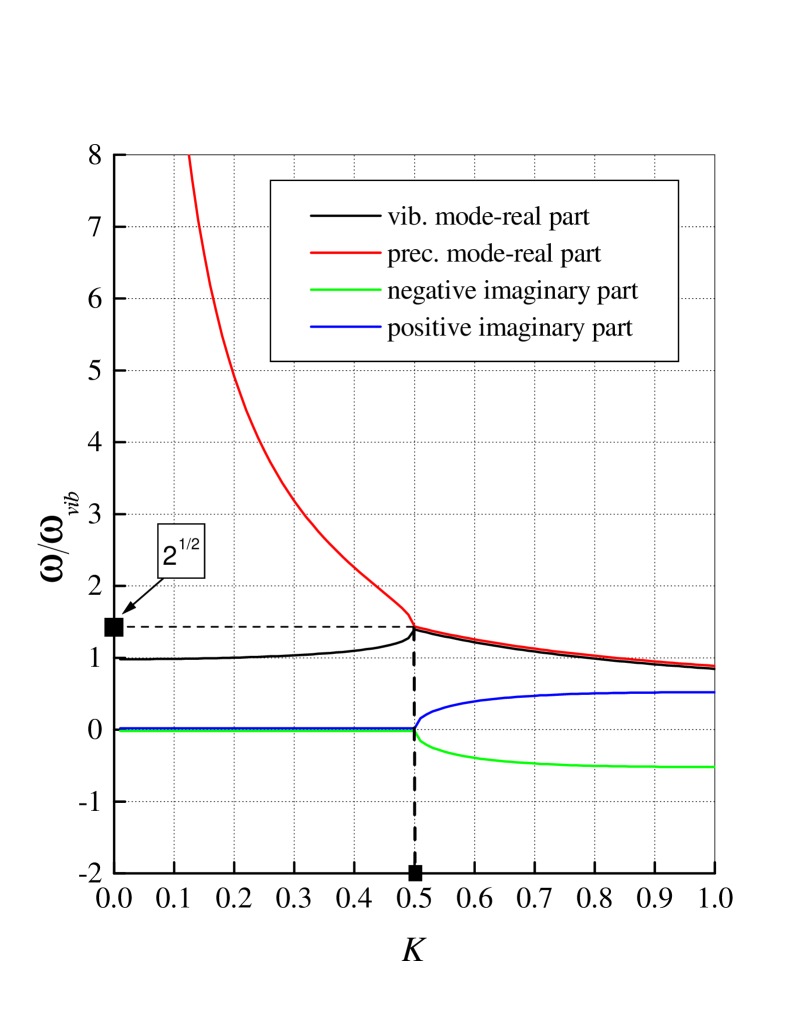
Figure 1: Real and imaginary parts of the mode frequencies as a function of $K$.

3.3 The excitation energy of the modes.

The excitation energy of a given mode is defined as the difference between the energy of the mode and the energy of the stationary state,

$$e=-\mu\mathbf{\hat{n}}\cdot\mathbf{B+}\dfrac{1}{2}m\left(\dfrac{d\delta x}{dt}\right)^{2}-\mu B_{0}.$$ (20)

Note that the energy is bilinear in the coordinates and hence, one cannot neglect the $\hat{z}$-component of the spin. Instead, one must set

$$\mathbf{\hat{n}\cdot\hat{z}=-}\sqrt{1-\left(\epsilon_{x}^{2}+\epsilon_{y}^{2}\right)}\mathbf{\simeq}-\left(1-\dfrac{1}{2}\left(\epsilon_{x}^{2}+\epsilon_{y}^{2}\right)\right).$$

Thus, the correct expression of the energy for small amplitudes is

$$e\simeq-\mu\left(\dfrac{1}{2}\left(\epsilon_{x}^{2}+\epsilon_{y}^{2}\right)B_{0}+B_{\perp}^{\prime}\delta x\epsilon_{y}\right)\mathbf{+}\dfrac{1}{2}m\left(\dfrac{d\delta x}{dt}\right)^{2}.$$ (21)

In this expression, the modes have to be written in real form,

$$\delta x\left(t\right)=\dfrac{B_{0}}{B_{\perp}^{\prime}}\left(\dfrac{\omega_{vib}}{\omega}\right)^{2}A\cos\left(\omega t\right),$$ (22)

$$\epsilon_{x}\left(t\right)=-K\dfrac{\omega}{\omega_{vib}}A\sin\left(\omega t\right),$$ (23)

$$\epsilon_{y}\left(t\right)=-A\cos\left(\omega t\right).$$ (24)

Substituting Eqs.(22), (23) and (24) into Eq.(21) and using Eq.(13) one finds that

$$\dfrac{e}{\mu B_{0}}=\dfrac{2\omega_{vib}^{2}-\omega^{2}}{2\omega^{2}}A^{2}.$$ (25)

Using Eq.(19) we conclude that for $0<K<0.5$, the excitation energy of the vibrational mode is positive while the excitation energy of the precessional mode is always negative. At the point $K=0.5$, where the two modes coalesce, the excitation energy vanishes. We will further refer to these observations in the following section.

3.4 The effect of viscous friction.

When friction is introduced into the system, the equations of motion become

$$m\dfrac{d^{2}x}{dt^{2}}=\mu\dfrac{\partial}{\partial x}\left(\mathbf{\hat{n}\cdot B}\right)-r_{t}\dfrac{dx}{dt}$$ (26)

and

$$S\dfrac{d\mathbf{\hat{n}}}{dt}=\mu\mathbf{\hat{n}\times B-}r_{p}\mathbf{\hat{n}\times}\dfrac{d\mathbf{\hat{n}}}{dt}\text{,}$$ (27)

where $r_{t}$ and $r_{p}$ are translational and precessional friction coefficients, respectively. The second term on the right-hand side of Eq.(27) is the spin-damping contributed by the change in the direction of the spin from $\mathbf{\hat{n}}$ to $\mathbf{\hat{n}+}d\mathbf{\hat{n}}$. Since, by definition, $\mathbf{\hat{n}}$ is a unit vector, $d\mathbf{\hat{n}}$ is perpendicular to $\mathbf{\hat{n}}$. Thus, $\Omega_{\perp}=\left|d\mathbf{\hat{n}/}dt\right|$ is the angular velocity associated with the change of $\mathbf{\hat{n}}$. Since the direction of $\Omega_{\perp}$ must be perpendicular to both $d\mathbf{\hat{n}}$ and $\mathbf{\hat{n}}$ we form the cross product $\mathbf{\Omega}_{\bot}=\mathbf{\hat{n}\times}\left(d\mathbf{\hat{n}/}dt\right)$ which incorporates both the correct value and the right direction. Multiplying $\mathbf{\Omega}_{\bot}$ by $r_{p}$ yields the spin-damping term.

To first order in $r_{r}$ and $r_{t}$ the secular equation in this case is given by

$$K^{2}\omega_{n}^{4}-\omega_{n}^{2}-2i\omega_{n}^{3}K\frac{r_{p}}{S}+i\frac{\omega_{n}^{3}}{S}\left(\dfrac{B_{0}}{B_{\perp}^{\prime}}\right)^{2}r_{t}K^{3}-i\omega_{n}\left(\dfrac{B_{0}}{B_{\perp}^{\prime}}\right)^{2}r_{t}\frac{K}{S}+1+i\omega_{n}K\frac{r_{p}}{S}=0$$ (28)

where we defined

$$\omega_{n}\equiv\dfrac{\omega}{\omega_{vib}}$$

to make the expression simple. Let $\omega_{n,0}$ be the eigenfrequencies $\omega_{n}$ of the frictionless problem, given by Eq.(13). When adding a small friction to the problem, the eigenfrequencies will change by a small amount $\delta\omega_{n}$. We find an approximate expression for $\delta\omega_{n}$ by expanding Eq.(28) around $\omega_{n,0}$ to first order in $\delta\omega_{n}$ and making use of Eq.(13). This gives

$$\delta\omega_{n}=\dfrac{iK}{2S}\left(\dfrac{r_{p}\omega_{n,0}^{2}\left(2\omega_{n,0}^{2}-1\right)+r_{t}\left(B_{0}/B_{\perp}^{\prime}\right)^{2}}{\omega_{n,0}^{2}-2}\right)+\mathcal{O}\left(r^{2}\right).$$ (29)

Eq.(29) has an interesting consequence: From Eq.(19) we find that the numerator in Eq.(29) is positive for both modes while the denominator is negative for the vibrational mode and positive for the precessional mode. We therefore conclude that friction, either translational or precessional, stabilizes the vibrational motion and, simultaneously, destabilizes the precessional motion. The system all together becomes of course, unstable.

The fact that spin damping leads to an exponential growth of the fast mode is no surprise in view of its negative excitation energy. Also, the exponential decay of the slow mode due to translational friction is to be expected on account of its positive excitation energy. What is important is the fact that due to the coupling between translation and precession, translational friction causes an exponential growth of the fast mode, with a growth time which, compared to the effect of spin damping, is smaller by a factor of $r_{t}K^{2}S^{2}/\mu mr_{p}B_{0}^{2}$ in the limit of small $K$.

4 Quantum-mechanical analysis.

4.1 The Hamiltonian and its diagonalized form.

In this section we consider the problem of a neutral particle with spin $S=\hbar/2$ in a 1D inhomogeneous magnetic field from a quantum-mechanical point of view. Unlike the classical analysis, in which the derivation was valid for any value of the adiabaticity parameter $K$, we concentrate here on the behavior of the system when $K$ is small. We choose to analyze the case of a spin $1/2$ particle because this case already shows the essentials of the quantum-mechanical problem.

Now, it is convenient to express the dependence of the magnetic field on $x$ in terms of its amplitude $B(x)$ and its direction $\theta(x)$ with respect to the $\mathbf{\hat{z}}$ axis. Thus, Eq.(2) is rewritten as

$$\mathbf{B}=B\left(x\right)\left(\sin\left[\theta\left(x\right)\right]\mathbf{\hat{y}}+\cos\left[\theta\left(x\right)\right]\mathbf{\hat{z}}\right)$$ (30)

where

$$B\left(x\right) =B\sqrt{1+\left(\dfrac{B_{\bot}^{\prime}x}{B_{0}}\right)^{2}}\text{ ,}$$ (31)

$$\theta\left(x\right) =\arctan\left(\dfrac{B_{\bot}^{\prime}x}{B_{0}}\right).$$

The time-independent Schrödinger equation for this system is

$$\left[\frac{-\hbar^{2}}{2m}\dfrac{\partial^{2}}{\partial x^{2}}-\mu B(x)\left(\sin\left[\theta\left(x\right)\right]\hat{\sigma}_{y}+\cos\left[\theta\left(x\right)\right]\hat{\sigma}_{z}\right)\right]\Psi\left(x\right)=E\Psi\left(x\right)$$ (32)

where $\hat{\sigma}_{y}$ and $\hat{\sigma}_{z}$ are the Pauli matrices given by

$$\begin{array}[c]{cc}\hat{\sigma}_{y}=\left(\begin{array}[c]{cc}0&-i\\ i&0\end{array}\right)\text{ ,}&\hat{\sigma}_{z}=\left(\begin{array}[c]{cc}1&0\\ 0&-1\end{array}\right),\end{array}$$

$E$ is the eigenenergy, and $\Psi$ is the two-component spinor

$$\Psi=\left(\begin{array}[c]{c}\psi_{\uparrow}\left(x\right)\\ \psi_{\downarrow}\left(x\right)\end{array}\right).$$ (33)

In matrix form Eq.(32) becomes

$$\left(H_{K}+H_{M}\right)\left(\begin{array}[c]{c}\psi_{\uparrow}\left(x\right)\\ \psi_{\downarrow}\left(x\right)\end{array}\right)=E\left(\begin{array}[c]{c}\psi_{\uparrow}\left(x\right)\\ \psi_{\downarrow}\left(x\right)\end{array}\right)$$ (34)

where $H_{K}$ and $H_{M}$, given by

$$H_{K} \equiv\dfrac{-\hbar^{2}}{2m}\left(\begin{array}[c]{cc}\dfrac{\partial^{2}}{\partial x^{2}}&0\\ 0&\dfrac{\partial^{2}}{\partial x^{2}}\end{array}\right)$$ (37)

$$H_{M} \equiv\mu B\left(x\right)\left(\begin{array}[c]{cc}-\cos\left[\theta\left(x\right)\right]&i\sin\left[\theta\left(x\right)\right]\\ -i\sin\left[\theta\left(x\right)\right]&\cos\left[\theta\left(x\right)\right]\end{array}\right),$$ (40)

are the kinetic part and the magnetic part of the Hamiltonian $H$, respectively.

In order to diagonalize the magnetic part of the Hamiltonian, we make a local passive transformation of coordinates on the wave function such that the spinor is expressed in a new coordinate system whose $\mathbf{\hat{z}}$ axis coincides with the direction of the magnetic field at the point $x$. We denote by $R\left(x\right)$ the required transformation and set $\Psi^{\prime}=R\Psi$. Thus, $\Psi^{\prime}$ represent the same direction of the spin as before the transformation but using the new coordinate system. The Hamiltonian in this newly defined system is clearly given by $RHR^{-1}$. In the case of the magnetic field given in Eq.(30), the required operation is a rotation by an angle $\theta\left(x\right)$ around the $\mathbf{-\hat{x}}$ axis. The operator that affects the wave function in this manner is [16]

$$R=\exp\left[-i\dfrac{\theta}{2}\hat{\sigma}_{x}\right]=\cos\left(\theta/2\right)-i\hat{\sigma}_{x}\sin\left(\theta/2\right),$$

while its inverse is given by

$$R^{-1}=\exp\left[i\dfrac{\theta}{2}\hat{\sigma}_{x}\right]=\cos\left(\theta/2\right)+i\hat{\sigma}_{x}\sin\left(\theta/2\right).$$

It is easily verified that the transformation indeed diagonalizes the magnetic part of the Hamiltonian,

$$RH_{M}R^{-1}=-\mu B\left(x\right)\hat{\sigma}_{z}.$$

For the kinetic part we find

$$RH_{K}R^{-1}=-\dfrac{\hbar^{2}}{2m}\left[\dfrac{\partial^{2}}{\partial x^{2}}-\dfrac{1}{4}\left(\dfrac{d\theta}{dx}\right)^{2}+i\left(\dfrac{d\theta}{dx}\dfrac{\partial}{\partial x}+\dfrac{1}{2}\dfrac{d^{2}\theta}{dx^{2}}\right)\hat{\sigma}_{x}\right].$$

Note that $i\left(\dfrac{d\theta}{dx}\dfrac{\partial}{\partial x}+\dfrac{1}{2}\dfrac{d^{2}\theta}{dx^{2}}\right)\hat{\sigma}_{x}$ is Hermitian.

Thus, the Hamiltonian of the system in the rotated frame may be written as

$$H=H_{diag}+H_{int}$$ (41)

where

$$H_{diag} =-\dfrac{\hbar^{2}}{2m}\left[\dfrac{\partial^{2}}{\partial x^{2}}-\dfrac{1}{4}\left(\dfrac{d\theta}{dx}\right)^{2}\right]-\mu B\left(x\right)\hat{\sigma}_{z}$$ (42)

$$H_{int} =-i\dfrac{\hbar^{2}}{2m}\left(\dfrac{d\theta}{dx}\dfrac{\partial}{\partial x}+\dfrac{1}{2}\dfrac{d^{2}\theta}{dx^{2}}\right)\hat{\sigma}_{x}.$$

The first part of the Hamiltonian $H_{diag}$ is diagonal. It contains the kinetic part $\sim\partial^{2}/\partial x^{2}$, a term whose form is $\mp$ $\mu B(x)$ which is to be identified as the adiabatic effective potential, and a term $\sim\left(d\theta/dx\right)^{2}$ which appear due to the rotation. The second part of the Hamiltonian $H_{int}$ contains only non-diagonal components. These will be shown to be of order $\mathcal{O}\left(K\right)$ and hence may be regarded as a small perturbation. We proceed to find the eigenstates of $H_{diag}$.

4.2 Stationary states of $H_{diag}$.

Since $H_{diag}$ is diagonal, the two spin states of the wavefunction are decoupled. We then seek a solution of the form

$$\Psi_{\downarrow}=\left(\begin{array}[c]{c}0\\ \psi_{\downarrow}(x)\end{array}\right)\text{ ; }E=E_{\downarrow},$$ (43)

referred to as the spin-down state, and another solution

$$\Psi_{\uparrow}=\left(\begin{array}[c]{c}\psi_{\uparrow}(x)\\ 0\end{array}\right)\text{ ; }E=E_{\uparrow},$$ (44)

which we call the spin-up state.

The equation for the non-vanishing component of the spin-down state is given by

$$\left[-\dfrac{\hbar^{2}}{2m}\left(\dfrac{\partial^{2}}{\partial x^{2}}-\dfrac{1}{4}\left(\dfrac{d\theta}{dx}\right)^{2}\right)+\mu B\left(x\right)\right]\psi_{\downarrow}=E_{\downarrow}\psi_{\downarrow},$$ (45)

whereas the equation for the non-vanishing component of the spin-up state is

$$\left[-\dfrac{\hbar^{2}}{2m}\left(\dfrac{\partial^{2}}{\partial x^{2}}-\dfrac{1}{4}\left(\dfrac{d\theta}{dx}\right)^{2}\right)-\mu B\left(x\right)\right]\psi_{\uparrow}=E_{\uparrow}\psi_{\uparrow}.$$ (46)

We now show that in the limit of small $K$ we can neglect the term $\sim\left(d\theta/dx\right)^{2}$ in both Eq.(45) and Eq.(46): We compare the order of magnitude of the term $\mu B\left(x\right)$ to that of the term $\hbar^{2}\left(d\theta/dx\right)^{2}/8m$. Using Eq.(31) it can be easily shown that the maximum value of $d\theta/dx$ is $B_{\bot}^{\prime}/B_{0}$ whereas the minimum value of $\mu B\left(x\right)$ is $\mu B_{0}$. Thus,

$$\dfrac{\left.\mu B\left(x\right)\right|_{\text{min}}}{\left(\dfrac{\hbar^{2}}{8m}\left(\dfrac{d\theta}{dx}\right)_{\text{max}}^{2}\right)}=\dfrac{8\mu mB_{0}^{3}}{\left(B_{\bot}^{\prime}\right)^{2}\hbar^{2}}=\frac{2}{K^{2}},$$

and we reach the conclusion that when $K$ is small enough we can neglect the term $\sim(d\theta/dx)^{2}$. Under this approximation, Eqs.(45) and (46) simplify to

$$\left[-\dfrac{\hbar^{2}}{2m}\dfrac{\partial^{2}}{\partial x^{2}}+\mu B\left(x\right)\right]\psi_{\downarrow}=E_{\downarrow}\psi_{\downarrow}$$ (47)

and

$$\left[-\dfrac{\hbar^{2}}{2m}\dfrac{\partial^{2}}{\partial x^{2}}-\mu B\left(x\right)\right]\psi_{\uparrow}=E_{\uparrow}\psi_{\uparrow}.$$ (48)

The approximate solutions of these equations are outlined in the next two subsections.

4.2.1 Stationary spin-down states.

Eq.(47) represents a particle in a symmetric attractive potential. If the extent of the wave function is small enough, we can expand $B\left(x\right)$ to second order in $x$

$$B\left(x\right)\simeq B_{0}\left[1+\dfrac{1}{2}\left(\dfrac{B_{\bot}^{\prime}x}{B_{0}}\right)^{2}\right]$$ (49)

and apply the well-known solution of a harmonic oscillator in one dimension. We now derive the condition for which this approximation is valid: We recall that the ground-state wave function of the harmonic oscillator is given by[17]

$$\psi_{\downarrow}\left(x\right)=\left(\dfrac{m\omega_{vib}}{\pi\hbar}\right)^{1/4}e^{-\dfrac{2m\omega_{vib}x^{2}}{\hbar}}.$$ (50)

The extent of this wave function over which it changes appreciably is given by

$$\Delta x_{\downarrow}\sim\sqrt{\dfrac{\hbar}{2m\omega_{vib}}},$$ (51)

whereas the extent over which $\mu B\left(x\right)$ changes significantly (see Eq.(31)) is

$$\Delta x_{\mu B}\sim B_{0}/B_{\bot}^{\prime}.$$ (52)

Thus, the ratio between these two length scales is

$$\dfrac{\Delta x_{\downarrow}}{\Delta x_{\mu B}}\sim\sqrt{\dfrac{\hbar\left(B_{\bot}^{\prime}\right)^{2}}{2m\omega_{vib}^{2}B_{0}^{2}}}\sim\sqrt{K}.$$ (53)

We therefore conclude that when $K$ is small enough, the harmonic approximation is justified. The wave function $\psi_{\downarrow}\left(x\right)$, given by Eq.(50), then represents the lowest possible bound state for this system. This state corresponds to a trapped particle. The energy of this state is clearly

$$E_{\downarrow}=\mu B_{0}+\frac{\hbar}{2}\omega_{vib}=\mu B_{0}\left(1+K\right)\simeq\mu B_{0},$$ (54)

while its full spinor representation is

$$\Psi_{\downarrow}=\left(\begin{array}[c]{c}0\\ \left(\dfrac{m\omega_{vib}}{\pi\hbar}\right)^{1/4}e^{-\dfrac{2m\omega_{vib}x^{2}}{\hbar}}\end{array}\right).$$ (55)

4.2.2 Stationary spin-up states.

Eq.(48) describes a particle in a repulsive potential. It corresponds to an unbounded state representing an untrapped particle. In this case there is a continuum of states, each with its own energy. As we are interested in non-radiative decay, we focus on finding a solution with an energy which is equal to the energy found for the trapped state, that is

$$E_{\uparrow}=E_{\downarrow}\simeq\mu B_{0}.$$ (56)

Since $H_{diag}$ is symmetric under $x\rightarrow-x$, to each energy in the continuous spectrum there belongs one state with even parity and one state with odd parity. Further, $H_{int}$ connects states with opposite parity only. Therefore, since the spin-down ground state is even in $x$, we need the spin-down state with odd parity.

When evaluating the lifetime in the next section, we compute the matrix element of $H_{int}$ between the states $\psi_{\uparrow}(x)$ and $\psi_{\downarrow}(x)$. Thus, most of the contribution to this integral comes from the region in $x$ where $\psi_{\downarrow}(x)$ is substantial. According to Eq.(53), $\mu B(x)$ changes very little in this range and, as a first approximation, we may take the potential in this region as uniform,

$$\mu B(x)\simeq\mu B_{0}$$ (57)

in Eq.(48), and then its solution becomes

$$\psi_{\uparrow}(x)=C\sin\left(\dfrac{\sqrt{4m\mu B_{0}}}{\hbar}x\right),$$ (58)

with the full spinor representation

$$\Psi_{\uparrow}(x)=\left(\begin{array}[c]{c}C\sin\left(\dfrac{\sqrt{4m\mu B_{0}}}{\hbar}x\right)\\ 0\end{array}\right).$$ (59)

The approximate wave function given in Eq.(58) is periodic near the origin, and has a period of

$$\Delta x_{\uparrow}=\dfrac{\pi\hbar}{\sqrt{\mu mB_{0}}}.$$ (60)

Comparing it to $\Delta x_{\downarrow}$ given in Eq.(51), we find that

$$\dfrac{\Delta x_{\uparrow}}{\Delta x_{\downarrow}}\sim\sqrt{K},$$ (61)

which shows that, when $K\ll 1$, the wavefunction $\psi_{\uparrow}\left(x\right)$ executes many oscillations in the region where $\psi_{\downarrow}\left(x\right)$ is appreciable.

4.3 The lifetime.

To evaluate the lifetime $T_{esc}$ of the particle in its trapped state, which is the average time it takes for the particle to escape, we calculate the transition rate from the bound state given by Eq.(55), to the unbounded state Eq.(59), according to Fermi’s golden rule[19]. Thus,

$$\dfrac{1}{T_{esc}}=\dfrac{2\pi}{\hbar}\left|H_{\downarrow,\uparrow}\right|^{2}g(E_{\uparrow})$$ (62)

where

$$H_{\downarrow,\uparrow}={\displaystyle\int\limits_{-\infty}^{+\infty}}\Psi_{\downarrow}^{\dagger}H_{int}\Psi_{\uparrow}dx={\displaystyle\int\limits_{-\infty}^{+\infty}}dx\psi_{\downarrow}^{\ast}\left(x\right)\left(\dfrac{\hbar^{2}}{2m}\right)\left(\dfrac{i}{2}\dfrac{d^{2}\theta}{dx^{2}}+i\dfrac{d\theta}{dx}\dfrac{\partial}{\partial x}\right)\psi_{\uparrow}\left(x\right)$$ (63)

is the matrix element of $H_{int}$ Eq.(42) between $\Psi_{\downarrow}$ and $\Psi_{\uparrow}$, and $g(E_{\uparrow})$ is the density of the final states at energy $E_{\uparrow}$.

Using Eq.(58) and Eq.(31) we find that

$$\dfrac{\dfrac{i}{2}\dfrac{d^{2}\theta}{dx^{2}}\psi_{\uparrow}}{\dfrac{d\theta}{dx}\dfrac{\partial\psi_{\uparrow}}{\partial x}}\sim\dfrac{\left(\dfrac{B_{\bot}^{\prime}}{B_{0}}\right)^{2}}{\dfrac{B_{\bot}^{\prime}}{B_{0}}\left(\dfrac{\sqrt{4m\mu B_{0}}}{\hbar}\right)}\sim K.$$

Thus, when $K$ is small we may neglect the contribution of $d^{2}\theta/dx^{2}$ to the integral Eq.(63) and then we find that

$$H_{\downarrow,\uparrow}=\dfrac{i\hbar^{2}}{2m}{\displaystyle\int\limits_{-\infty}^{+\infty}}dx\psi_{\downarrow}^{\ast}\left(x\right)\dfrac{d\theta}{dx}\dfrac{\partial\psi_{\uparrow}\left(x\right)}{\partial x}.$$ (64)

The integrand in Eq.(64) consists of a product of three functions: The function $\psi_{\downarrow}^{\ast}$ whose ‘width’ is about $\Delta x_{\downarrow}$ (given in Eq.(51)) around the origin, the function $d\theta/dx$ whose extent around the origin $\Delta x_{\mu B}$ is roughly $\sqrt{1/K}$ larger than $\Delta x_{\downarrow}$ and the function $\partial\psi_{\uparrow}/\partial x$ which is a periodic function with a characteristic period $\Delta x_{\uparrow}$ which is $\sqrt{K}$ smaller than $\Delta x_{\downarrow}$. This suggests that we can approximate the integral in Eq.(64) by substituting $d\theta/dx$ for its value at $x=0$,

$$\dfrac{d\theta}{dx}\simeq\dfrac{B_{\bot}^{\prime}}{B_{0}}.$$ (65)

Substituting Eqs.(65), (50) and (58) into Eq.(64) gives

$$H_{\downarrow,\uparrow}\simeq i\dfrac{\hbar}{2m^{3/4}}C\sqrt{\dfrac{2\mu\left(B_{\bot}^{\prime}\right)^{2}}{B_{0}}}\left(\dfrac{\pi\hbar}{\omega_{vib}}\right)^{1/4}\exp\left[-\dfrac{\mu B_{0}}{2\hbar\omega_{vib}}\right],$$ (66)

where we have used the definite integral

$${\displaystyle\int\limits_{-\infty}^{+\infty}}e^{-ax^{2}}\cos\left(bx\right)dx=\sqrt{\dfrac{\pi}{a}}\exp\left[-\dfrac{b^{2}}{4a}\right].$$ (67)

When Eq.(66) is substituted into Eq.(62) the term $\left|C\right|^{2}g(E_{\uparrow})$ appears. This term can be calculated by temporarily introducing suitable boundary conditions: Assume that the system is bounded by an infinite potential wall at $x=\pm L/2$, the length $L$ being large compared to $\Delta x_{\downarrow}$ yet small when compared to $\Delta x_{\mu B}$. In this case, the uniform potential approximation still holds, and we may use the well-known result for the density of states for a particle in a 1D infinite potential well,

$$g(E_{\uparrow}=\mu B_{0})=\sqrt{\dfrac{mL^{2}}{4\mu B_{0}\pi^{2}\hbar^{2}}}.$$ (68)

The evaluation of the normalization constant $C$ gives

$$\left|C\right|^{2}=2/L,$$ (69)

and therefore

$$\left|C\right|^{2}g(E_{\uparrow})=\sqrt{\dfrac{m}{\mu B_{0}\pi^{2}\hbar^{2}}}.$$ (70)

Finally, using Eqs.(70) and (66) inside Eq.(62) gives

$$T_{esc}=\dfrac{1}{\omega_{vib}}\sqrt{\dfrac{1}{2\pi K}}\exp\left[\dfrac{1}{2K}\right]=T_{vib}\dfrac{1}{\sqrt{\left(2\pi\right)^{3}K}}\exp\left[\dfrac{1}{2K}\right],$$ (71)

where $T_{vib}=2\pi/\omega_{vib}$ is the period of classical oscillations inside the trap.

Looking back at the calculation of the matrix element, Eq.(66), one realizes that for small $K$ the wave function $\psi_{\uparrow}$ oscillates strongly in the region where the wave function $\psi_{\downarrow}$ is essentially different from zero. Thus, successive subintervals compensate each other very effectively, and it is possible that the regions $\left|x\right|>\Delta x_{\downarrow}$ where the $x$-dependence of the potential becomes important, contribute more effectively to the integral than the simple estimates indicate. We have therefore carried out a more accurate calculation, using the WKB approximation[18], which takes the $x$-dependence of the potential into account. The calculation, which is given in the Appendix, yields the result

$$T_{esc}\simeq\dfrac{1}{\omega_{vib}}\dfrac{33}{32}\sqrt{\dfrac{1}{2\pi K}}\exp\left[\dfrac{2}{K}\arctan\left(\dfrac{1}{4}\right)\right]$$ (72)

which does indeed differ from Eq.(71) not only by the prefactor, being unity in Eq.(71) and $33/32$ in Eq.(72), but even by the exponent which is $0.5$ in Eq.(71) and $2\arctan\left(1/4\right)\simeq 0.\,\allowbreak 489\,96$ in Eq.(72).

5 Discussion.

Summarizing all we have found we conclude that the problem we have studied has three important time scales: The shortest time scale is $T_{prec}$, which is the time required for one precession of the spin around the axis of the local magnetic field. The intermediate time scale is $T_{vib}=T_{prec}/K$, which is the time required to complete one cycle of the center of mass around the center of the trap. These two time scales appear both in the classical and the quantum-mechanical analysis. The longest time scale (provided $K$ is small) $T_{esc}$, which is not present in the classical problem, is the time it takes for the particle to escape from the trap.

Whereas the classical analysis yields an upper bound of $K=0.5$ for trapping to occur, no such sharp bound exists in the quantum-mechanical analysis. This is related to the fact that one cannot associate an effective potential well with a finite barrier with the system. Nevertheless it is interesting to compare the classical bound with the value of $K$ for which the exponent in the expression for the quantum-mechanical lifetime becomes equal to $1$: For the uniform-field approximation, Eq.(71), the two values happen to agree exactly, and in the WKB approximation, Eq.(72), they differ only by a small amount. Thus, the quantum-mechanical condition for trapping to occur is essentially the same as the classical condition.

As an example, we apply our results to the case of a neutron and an atom trapped with a field $B_{0}=100$ Oe and $B_{0}/B_{\bot}^{\prime}=10$cm. These parameters correspond to typical traps used in Bose-Einstein condensation experiments[7]. The results, being correct to within an order of magnitude, are outlined in the following table:

$$\begin{array}[c]{c}B_{0}=100\text{ Oe}\\ B_{0}/B_{\bot}^{\prime}=10\text{cm}\end{array}$$

Neutron Atom

gr

emu

sec

sec

sec

We note that in both cases $K$ is very small compared to $1$. Consequently, the calculated lifetime of the particle in the trap is extremely large, suggesting that the particle (either neutron or atom) is tightly trapped in this field.

Though the toy model presented in this paper is very simple, preliminary studies[21] show that behavior similar to what we found in this model trap appears also in more realistic magnetic traps such as those used in Bose-Einstein condensation experiments. For example, a similar analysis of a two-dimensional Ioffee trap[2] shows similar behavior when the classical analysis and quantum-mechanical analysis are compared, but in this case we find that $T_{esc}\sim\exp\left[2/K^{3}\right]$.

The problem studied in this paper deals with a spin $1/2$ particle. Though this fact has little influence on the solution of the classical problem, the extension to higher spin values complicates the analysis of the quantum-mechanical problem. In this case one has to deal with a ($2S+1$)-component spinor, and the interaction Hamiltonian does no longer connect the ($-S$)-state to the ($+S$)-state, but only to the ($-S+1$) and ($-S+2$) states which for $S\geq 5/2$ will still be trapped.

Appendix A Calculation of $\psi_{\uparrow}$ and $T_{esc}$ by the WKB method.

In this appendix, we outline the solution of Eq.(48) by the WKB approximation and calculate the resulting lifetime. The validity of the WKB approximation is guaranteed by the following argument: We first note that, for $E_{\uparrow}=\mu B_{0}$, the local de-Broglie wavelength $\lambda\left(x\right)$ is given by

$$\lambda\left(x\right)=\dfrac{2\pi\hbar}{\left.p_{E_{\uparrow}}(x)\right|_{@E_{\uparrow}=\mu B_{0}}}$$ (73)

where

$$p_{E_{\uparrow}}(x)=\sqrt{2m(E_{\uparrow}+\mu B\left(x\right))}\simeq\sqrt{2m\mu B_{0}\left(2+\dfrac{1}{2}\left(\dfrac{B_{\perp}^{\prime}x}{B_{0}}\right)^{2}\right)}$$ (74)

is the classical momentum of the particle. Thus, the rate of change of $\lambda$ over $x$ is

$$\left|\dfrac{d\lambda}{dx}\right|=2\pi\hbar\mu m\left[2m(\mu B_{0}+\mu B\left(x\right)\right]^{-3/2}\left|\dfrac{\partial B(x)}{\partial x}\right|.$$ (75)

Its maximum value is given by

$$\left|\dfrac{d\lambda}{dx}\right|_{\text{max}}\sim\dfrac{\mu m\hbar}{\left[2m(\mu B_{0}+\mu B_{0})\right]^{3/2}}B^{\prime}\sim\sqrt{\dfrac{\hbar^{2}\left(B_{\bot}^{\prime}\right)^{2}}{\mu mB_{0}^{3}}}\sim K.$$ (76)

Hence, in the adiabatic approximation, where $K\ll 1$, the validity condition of the WKB approximation $\left|d\lambda/dx\right|\ll 1$ is satisfied.

In this approximation the wavefunction $\psi_{\uparrow}(x)$ corresponding to the energy $E_{\uparrow}$ is given by[18]

$$\psi_{\uparrow}(x)=\dfrac{D}{\sqrt{\left|p_{E_{\uparrow}}(x)\right|}}\sin\left(\dfrac{1}{\hbar}{\displaystyle\int\limits_{a}^{x}}p_{E_{\uparrow}}(x^{\prime})dx^{\prime}\right),$$ (77)

where $a$, the lower limit of the integration, is yet undetermined.

We still need to evaluate the product $\left|D\right|^{2}g(E_{\uparrow}=\mu B)$ which appears when calculating $T_{esc}$ by Eq.(62). We therefore temporarily introduce boundary conditions by assuming that the system is bounded by an infinite potential wall at $x=\pm L/2$. Thus, by setting $a=-L/2$ the boundary condition at $x=-L/2$ is automatically satisfied. We note that we are looking for a highly excited state $\psi_{\uparrow}$ and we consider the eigenstate corresponding to the nearest higher energy $E_{\uparrow}+\Delta E$. The latter must fulfill the requirement that the phase of $\psi$ at $x=L/2$ changes by $\pi$ when going from $E_{\uparrow}$ to $E_{\uparrow}+\Delta E$. Thus,

$$\dfrac{1}{\hbar}\left[\int_{-L/2}^{L/2}p_{E_{\uparrow}+\Delta E}(x^{\prime})dx^{\prime}-\int_{-L/2}^{L/2}p_{E_{\uparrow}}(x^{\prime})dx^{\prime}\right]=\pi.$$ (78)

Since $E_{\uparrow}\gg\mu B(x)$ everywhere we may write the difference in Eq.(78) as a derivative

$$\dfrac{1}{\hbar}\Delta E\dfrac{\partial}{\partial E_{\uparrow}}\int_{-L/2}^{L/2}p_{E_{\uparrow}}(x^{\prime})dx^{\prime}=\pi.$$ (79)

Using Eq.(74) we rewrite Eq.(79) as

$$\dfrac{1}{\hbar}\Delta E\int_{-L/2}^{L/2}\dfrac{m}{p_{E_{\uparrow}}(x^{\prime})}dx^{\prime}=\pi.$$ (80)

Normalization of the wavefunction Eq.(77), gives on the other-hand

$$\int_{-L/2}^{L/2}\left|\psi_{\uparrow}(x)\right|^{2}dx \simeq\left|D\right|^{2}\int_{-L/2}^{L/2}\dfrac{1}{\left|p_{E_{\uparrow}}(x)\right|}\sin^{2}\left(\dfrac{1}{\hbar}{\displaystyle\int\limits_{-L/2}^{x}}p_{E_{\uparrow}}(x^{\prime})dx^{\prime}\right)dx$$ (81)

$$\simeq\dfrac{1}{2}\left|D\right|^{2}\int_{-L/2}^{L/2}\dfrac{1}{p_{E}(x)}dx=1,$$

where we have neglected the terms containing fast oscillations by replacing the $\sin^{2}()$ term by its average value $1/2$ . Substituting Eq.(81) into Eq.(80) gives

$$\left|D\right|^{2}\dfrac{1}{\Delta E}=\left|D\right|^{2}g(E_{\uparrow})=\dfrac{2m}{\pi\hbar}$$ (82)

where $g(E_{\uparrow})=1/\Delta E$ is the density of states at energy $E_{\uparrow}$.

To evaluate the integral in Eq.(64) we use the stationary phase method[20]. Using Eqs.(77), (50) and (65) we rewrite this integral as

$$H_{\uparrow,\downarrow}\simeq i\dfrac{\hbar^{2}}{2m}\int\psi_{\uparrow}^{\ast}\left(x\right)\dfrac{d\theta}{dx}\dfrac{\partial\psi_{\downarrow}}{\partial x}dx=I_{+}-I_{-}$$

where we have defined

$$I_{\pm}=A{\displaystyle\int\limits_{-\infty}^{+\infty}}dxg(x)\exp f_{\pm}(x),$$

$$A\equiv\dfrac{\hbar^{2}}{4m}\left(\dfrac{m\omega_{vib}}{2\pi\hbar}\right)^{1/4}\left(\dfrac{4m\omega_{vib}}{\hbar}\right)D\left(\dfrac{B_{\bot}^{\prime}}{B_{0}}\right),$$

$$g(x)\equiv\dfrac{x}{\sqrt{\left|p_{E_{\uparrow}}\left(x\right)\right|}},$$

and

$$f_{\pm}(x)\equiv-\dfrac{2m\omega_{vib}x^{2}}{\hbar}\pm\dfrac{i}{\hbar}{\displaystyle\int\limits_{0}^{x}}p_{E_{\uparrow}}\left(x^{\prime}\right)dx^{\prime}.$$ (83)

Note that the lower integration limit in $f_{\pm}\left(x\right)$ has been chosen as $0$ to make the function $\psi_{\uparrow}^{\ast}\left(x\right)$ antisymmetric under $x\rightarrow-x$.

We continue to work out $I_{+}$ first: According to the stationary phase approximation we should first find the point $x_{s}$ for which the phase $f_{+}(x)$ is stationary. This is accomplished by solving

$$\dfrac{\partial f_{+}}{\partial x}=\dfrac{\partial}{\partial x}\left[-\dfrac{2m\omega_{vib}x^{2}}{\hbar}+\dfrac{i}{\hbar}{\displaystyle\int\limits^{x}}p_{E_{\uparrow}}\left(x^{\prime}\right)dx^{\prime}\right]=0$$ (84)

for $x$. Using Eqs.(56) and (49) and after a few algebraic steps we find that the only solution to Eq.(84) is

$$x_{s}^{+}=i\sqrt{\dfrac{4}{17}}\dfrac{B_{0}}{B_{\bot}^{\prime}}.$$ (85)

Now we approximate the integral $I_{+}$ as

$$I_{+}=A{\displaystyle\int\limits_{-\infty}^{+\infty}}dxg(x)\exp\left[f_{+}(x)\right]\simeq Ag(x_{s}^{+})\sqrt{\dfrac{2\pi}{-f_{+}^{\prime\prime}(x_{s}^{+})}}\exp\left[f_{+}(x_{s}^{+})\right].$$ (86)

The evaluation of $f_{+}(x_{s}^{+})$ is performed in the following way:

$$f_{+}(x_{s}^{+}) =-\dfrac{2m\omega_{vib}\left(x_{s}^{+}\right)^{2}}{\hbar}+\dfrac{i}{\hbar}{\displaystyle\int\limits_{0}^{i\sqrt{4/17}B_{0}/B_{\perp}^{\prime}}}p_{E_{\uparrow}}\left(x\right)dx$$

$$=\dfrac{2m}{\hbar}\sqrt{\dfrac{\left(B_{\perp}^{\prime}\right)^{2}\mu}{mB_{0}}}\left(\sqrt{\dfrac{4}{17}}\dfrac{B_{0}}{B_{\perp}^{\prime}}\right)^{2}+\dfrac{i^{2}}{\hbar}{\displaystyle\int\limits_{0}^{\sqrt{4/17}B_{0}/B_{\perp}^{\prime}}}p_{E_{\uparrow}}\left(iy\right)dy$$

$$=\dfrac{2m}{\hbar}\sqrt{\dfrac{\left(B_{\perp}^{\prime}\right)^{2}\mu}{mB_{0}}}\left(\sqrt{\dfrac{4}{17}}\dfrac{B_{0}}{B_{\perp}^{\prime}}\right)^{2}-\dfrac{1}{\hbar}{\displaystyle\int\limits_{0}^{\sqrt{4/17}B_{0}/B_{\perp}^{\prime}}}\sqrt{2m\mu B_{0}\left(2-\dfrac{1}{2}\left(\dfrac{B_{\perp}^{\prime}y}{B_{0}}\right)^{2}\right)}dy$$

$$=-\sqrt{\dfrac{4\mu mB_{0}^{3}}{\left(B_{\perp}^{\prime}\right)^{2}\hbar^{2}}}\arcsin\left(\frac{1}{\sqrt{17}}\right)=-\dfrac{\arctan\left(1/4\right)}{K}$$

where we used the definite integral

$$\int_{0}^{y}\sqrt{a^{2}-x^{2}}dx=\dfrac{1}{2}y\sqrt{a^{2}-y^{2}}+\dfrac{1}{2}a^{2}\arcsin\left(\dfrac{y}{a}\right)\text{ ; for }y<a\text{.}$$

The term $f_{+}^{\prime\prime}(x_{s}^{+})$ is calculated straightforward with the result that

$$f_{+}^{\prime\prime}(x_{s}^{+}) =\sqrt{\dfrac{m\mu\left(B_{\bot}^{\prime}\right)^{2}}{B_{0}}}\left(-2-i\dfrac{1}{17\sqrt{1-1/17}}\right)$$ (87)

$$=-2\sqrt{\dfrac{m\mu\left(B_{\bot}^{\prime}\right)^{2}}{B_{0}}}\sqrt{\dfrac{1089}{1088}}\exp\left[i\arctan\left(\dfrac{\sqrt{17}}{136}\right)\right].$$

Substituting this together with $g(x_{s}^{+})$ and $f(x_{s}^{+})$ into Eq.(86) gives

$$I_{+} =iA\sqrt{\dfrac{B_{0}}{B_{\bot}^{\prime}}}\dfrac{\left(17\right)^{1/4}}{2}\sqrt{\dfrac{2\pi}{17}}\sqrt{\dfrac{B_{0}}{m\mu\left(B_{\bot}^{\prime}\right)^{2}}}$$ (88)

$$\times\left(\dfrac{1088}{1089}\right)^{1/4}\exp\left[-\dfrac{1}{K}\arctan\left(\dfrac{1}{4}\right)-\dfrac{i}{2}\arctan\left(\dfrac{\sqrt{17}}{136}\right)\right].$$

Likewise, a similar calculation for $I_{-}$ gives

$$x_{s}^{-} =-x_{s}^{+}$$

$$f_{-}(x_{s}^{-}) =f_{+}(x_{s}^{+})$$

$$f_{-}^{\prime\prime}(x_{s}^{-}) =f_{+}^{\prime\prime}(x_{s}^{+})$$

$$g(x_{s}^{-}) =-g(x_{s}^{+}),$$

leading to the result that

$$I_{-} =-iA\sqrt{\dfrac{B_{0}}{B_{\bot}^{\prime}}}\dfrac{\left(17\right)^{1/4}}{2}\sqrt{\dfrac{2\pi}{17}}\sqrt{\dfrac{B_{0}}{m\mu\left(B_{\bot}^{\prime}\right)^{2}}}$$ (89)

$$\times\left(\dfrac{1088}{1089}\right)^{1/4}\exp\left[-\dfrac{1}{K}\arctan\left(\dfrac{1}{4}\right)-\dfrac{i}{2}\arctan\left(\dfrac{\sqrt{17}}{136}\right)\right].$$

By repeating the steps that led to Eq.(71) we find that

$$T_{esc}=\dfrac{1}{\omega_{vib}}\dfrac{33}{32}\sqrt{\dfrac{1}{2\pi K}}\exp\left[\dfrac{2}{K}\arctan\left(\dfrac{1}{4}\right)\right].$$ (90)

References

- [1] A. L. Migdall, J. V. Prodan and W. D. Phillips, Phys. Rev. Lett., 54 (24), 2596-2599 (1985).
- [2] T. Bergeman, G. Erez, H. J. Metcalf, Phys. Rev. A., 35 (4), 1535-1546 (1987).
- [3] V. S. Bagnato et al., Phys. Rev. Lett., 58 (21), 2194-2197 (1987).
- [4] W. Petrich et al., Phys. Rev. Lett., 74 (17), 3352-3355 (1995).
- [5] D. Meacher, Physics World, 21-22 ( July 1995).
- [6] M. O. Mewes, M. R. Andrews, N. J. Van-Druten, D. M. Kurn, D. S. Durfee, W. Ketterle, Phys. Rev. Lett., 77(3), 416-419 (1996).
- [7] ‘Physics Today’, Aug. 1995, pp. 17-20.
- [8] The Levitron is available from ‘Fascinations’, 18964 Des Moines Way South, Seattle, WA 98148.
- [9] Hones et al., U.S. Patent Number: 5,404,062, Date of Patent: Apr. 4, 1995.
- [10] The U-CAS is available from Masudaya International Inc., 6-4, Kuramae, 2-Chome, Taito-Ku, Tokyo, 111 Japan.
- [11] M. V. Berry, Proc. R. Soc. Lond. A 452, 1207-1220 (1996).
- [12] S. Gov and S. Shtrikman, Proc. of the 19 IEEE Conv. in Israel, 184-187 (1996).
- [13] M. D. Simon, L. O. Heflinger and S. L. Ridgway, Am. J. Phys. 65 (4), 286-292 (1997).
- [14] S. Gov, S. Shtrikman and H. Thomas, Los-Alamos E-Print Archive, http://xxx.lanl.gov/, physics/9803020 (1998).
- [15] S. Earnshaw, Trans. Cambridge Philos. Soc. 7, 97-112 (1842).
- [16] ‘Quantum Mechanics’ by L. D. Landau and E. M. Lifshitz, Pergamon Press, 3 Ed., Ch. 8, Sec. 58, 213-214.
- [17] ‘Quantum Mechanics’ by E. Merzbacher, John Wiley & Sons., 2 Ed., Ch. 5, Sec. 3, 57-61.
- [18] ‘Quantum Mechanics’ by L. D. Landau and E. M. Lifshitz, Pergamon Press, 3 Ed., Ch. 8, Sec. 58 213-214.
- [19] ‘Quantum Mechanics’ by E. Merzbacher, John Wiley & Sons., 2 Ed., Ch. 18, Sec. 8, 475-481.
- [20] This method, also known as the method of steepest descent is described, for example, in ‘The mathematics of physics and chemistry’ by H. Margenau and G. M. Murphy, d. Van Norstad Co., Ch. 12, Sec. 10, 459-466.
- [21] S. Gov, S. Shtrikman and H. Thomas, to be published.