A CTMC study of collisions
between protons and $H_{2}^{+}$ molecular ions

Abstract

We study numerically collisions between protons and $H_{2}^{+}$ molecular ions at intermediate impact energies by using the Classical Trajectory Monte Carlo method (CTMC). Total and differential cross sections are computed. The results are compared with: a) the standard one electron–two nucleon scattering, and b) the quantum mechanical treatment of the $H^{+}-H^{+}_{2}$ scattering.

I Introduction

Ion–atom collisions represent one of the main fields of research in atomic physics, both experimental and theoretical. Currently, there is a great deal of studies about the collisions with electron transfer between ions and oriented atoms (i.e. with a preferred sense of circulation of the electron around the nucleus) and also between ions and aligned atoms (where the probability distribution of the electron is not spherical). The interest has been triggered by the development of experimental techniques which allow to prepare atoms in well defined states of low [1] or high quantum numbers $(n,l,m)$ [2] and, after scattering, to measure the final state of the system [3]. The very narrow phase space volume sampled by the electron allows a detailed study of the physical mechanisms occurring during the impact, which would not be otherwise transparent due to the averaging over the entire space of electronic configurations. Consequences of first order effects–spatial overlap and velocity matching–have been extensively studied with the above mentioned techniques, interpreted in the light of classical mechanics [4, 5] and sometimes compared with exact quantum calculations [6, 7]. A recent brief review about the latest developments in this field is given by Schippers [8], and some even more recent experimental and theoretical works can be found in [9].
Less attention has been paid to processes which involve more than one target nucleus: some studies of collisions between $H_{2}$ and bare ions are reported, for example, in [8, 10, 11, 12, 13], and the scattering $H^{+}$–$H_{2}^{+}$ is the subject of [14].
Calculations on these systems using quantum mechanics is far from being straightforward. By contrast, the application of classical methods, and in particular of the Classical Trajectory Monte Carlo method (CTMC) presents several advantages: The numerical complications introduced by solving the equations of motion for a few more particles are negligible. One may think, in comparison, to the problems which arise when attempting of solving the Schrödinger equation for three particles instead of two.
Since the original work of Abrines and Percival [15] the CTMC method has been one of the most successful techniques for studying the scattering between heavy charged particles at intermediate impact energies. Starting from the simple $H$–$H^{+}$ processes and from the calculation of simple total cross sections, the method has been refined so that nowadays it gives many detailed informations: Differential cross sections [16], which are ordinarily measured in experiments, and state–to–state transitions [17], which are especially useful for the research and development on thermonuclear fusion. The CTMC method has also been applied to more complex systems: Collisions involving more than an electron [18], requiring the inter-electronic correlation, have been, and still are [16, 19], a great challenge.

To our knowledge, until now CTMC has not been applied to polynuclear targets: In this work we do an investigation on this kind of process using the simplest target, the $H_{2}^{+}$ molecular ion. We aim to understand how and to which degree the complex structure of the target modifies the results of the scattering with respect to the standard two nucleons–one electron case.
In presence of a diatomic target the question of interference between the two scattering centres raises, and it has been faced within the quantum–mechanical formalism in Refs. [10, 11, 14]. In classical calculations one cannot speak of interference as in quantum ones; however a certain modification of the results due to the presence of a second target is likely to be expected.

The first problem one has to face is to obtain an equilibrium electron distribution function for the $H_{2}^{+}$ molecular ion. In Section II it is described how this has been dealt with in this work.

The results of the numerical simulations, expressed in the form of cross sections, are compared with the similar results for two nucleons scattering, and the differences are examined in Section III.

II Theory

In any CTMC calculation an important role is played by the choice of the initial conditions of the electron in the phase space. It is well known that, in the case of the ground state of hydrogen, extracting electron coordinates from a microcanonical distribution, $f({\bf r},{\bf p})=\delta(E-E_{1s})/8\pi^{3}$, yields the correct quantum mechanical momentum distribution [19]:

$$\tilde{\varrho}({\bf p})=N{p^{2}\over(p^{2}+2|E_{1s}|)^{4}}\quad,$$ (1)

where $E_{1s}=-0.5$ au (atomic units will be used unless otherwise stated), and $N$ the normalization factor. Obviously this relations holds also for hydrogen–like ions. On the other hand, the radial distribution is not reproduced satisfactorily. While no classical method can reproduce at the same time both the exact momentum and spatial distribution, some methods have been devised which allow to exactly reproduce the latter distribution at the expenses of the former (so called CTMC-r method, opposed to the CTMC-p method–see [20] ), or to yield an approximate–but rather good–description of both distributions (for more about the subject see the references quoted in [16] or [21]). In this work we have approximated the quantum mechanical electron wave function by a Linear Combination of Atomic Orbitals:

$$\psi({\bf r})={\psi_{1s}^{A}({\bf r})+\psi_{1s}^{B}({\bf r})\over\sqrt{2}}\;,$$ (2)

where $A$ and $B$ refer to the two protons which are placed initially with null velocity along the $z$ axis, at a distance $\pm z_{0}$ from the origin, with $z_{0}$ kept equal to 1 au, in accordance with the true equilibrium internuclear distance. With this choice the molecule has a cylindrical symmetry with respect to the $z$ axis. From a Fourier transform of Eq. (2) we get the momentum distribution function: since

$$\psi_{1s}^{A}({\bf r})+\psi_{1s}^{B}({\bf r})=\psi_{1s}({\bf r}-{\bf r}_{0})+\psi_{1s}({\bf r}+{\bf r}_{0})\quad,$$ (3)

where ${\bf r}_{0}=(0,0,z_{0})$, we obtain

$${\tilde{\psi}}({\bf p})={1\over(2\pi)^{3}}\int\;d{\bf r}\;\psi({\bf r})\;e^{-i{\bf p}\cdot{\bf r}}={1\over\sqrt{2}}\left(e^{-ip_{z}z_{0}}\tilde{\psi}_{1s}(p)+e^{ip_{z}z_{0}}\tilde{\psi}_{1s}(p)\right)\quad.$$ (4)

The probability density is better expressed in cylindrical coordinates

$$\tilde{\varrho}({\bf p})=2\pi p_{r}|\tilde{\psi}({\bf p})|^{2}=N^{\prime}{p_{r}\over(1+p_{r}^{2}+p_{z}^{2})^{4}}\cos^{2}(p_{z}z_{0})\quad,$$ (5)

where $p_{z},p_{r}$ are the projections of $\bf p$ along the $z$ axis and the radial direction in the x-y plane. $N^{\prime}$ is a normalization factor.

The probability density $\tilde{\varrho}$ is similar to a hydrogenic distribution (see Eq. 1) but for the factor $p_{r}\cos^{2}(p_{z}z_{0})$. This means that electron velocity is preferentially found within the x-y plane, where $p_{z}\simeq 0$.

The couples $p_{r}$, $p_{z}$ are picked up within a range $(0,p_{max})$ and generated according to the distribution of Eq. (5) with a rejection technique; $p_{max}$ is chosen great enough so that $\tilde{\varrho}(p_{r},p_{z})$ is negligible for $p_{r}^{2}+p_{z}^{2}>p_{max}^{2}$: in the computations $p_{max}=4.5$.

The choice of the spatial position of the electron follows a similar route. The position $\bf r$ is constrained to satisfy

$${p^{2}\over 2m_{e}}-{1\over|{\bf r}-{\bf r}_{0}|}-{1\over|{\bf r}+{\bf r}_{0}|}=E_{H_{2}^{+}}\quad,$$ (6)

where ${\bf r}_{0}=(0,0,z_{0})$ and $E_{H_{2}^{+}}\simeq-1.1$ au is the experimental quantity. $\bf r$ is characterized by the three numbers: the radial distance $r=|{\bf r}|$, the polar angle $\theta$ and the azimuthal angle $\phi$. Again, $r$ and $\cos(\theta)$ are chosen with a rejection technique within the ranges $(0,r_{max})$ and $(-1,1)$ respectively. $\phi$ does not explicitly appear in Eq. (6) and may be chosen uniformly in the interval $(0,2\pi)$.
The chosen distribution is not expected to be a stationary one for the classical system, so it is of interest to see how much it varies with time. In Figure 1 we plotted the contour of the distributions $\tilde{\varrho}(p_{z},p_{r})$ $\varrho(z,r)$ at $t=0$ and $t=5$, in absence of the projectile, from which one may see that the difference is not small but the essential features still remain so the choice of this distribution appears to be justified.

The projectile initial parameters are the velocity $v$, the impact parameter $b$ with respect of the centre of mass $O$ of the molecule, the azimuthal angle $\vartheta$ with respect to the molecule axis, and the initial distance $d$ from $O$. A sketch of the scattering configuration for the coplanar case (all the nuclei lying on the same plane) is shown in Figure 2. The projectile is then rotated out of the plane by a random angle between 0 and $2\pi$.

After having initialized all the four particles, the corresponding equations of the motions are numerically integrated in time until the nucleons are well far apart. In the computations $d$ is not a critical parameter as far as it is great enough to allow the target molecule and the projectile to be considered initially as non–interacting. After some trials a value of $d\simeq 20$ au was found to be reasonable. With given values for $b$, $v$ and $\vartheta$, a number $N$ of runs have been carried on, varying only the electron initial conditions. At the end of each collision one may find one of the following situations: 1) the original molecule remains intact; 2) it may be dissociated but the electron is still bound to one of the two nuclei; 3) the electron is bound to the projectile (we call this case ”charge transfer”); 4) the molecule may be broken and the electron be ionized. Each process $i$ (with $i=1,2,3,4$) happens $N_{i}$ times over the total $N$ runs, with corresponding probabilities

$$P_{i}(v,b,\vartheta)={N_{i}\over N}\quad.$$ (7)

The standard deviation error of $P_{i}$ is

$$\Delta P_{i}=\sqrt{{N-N_{i}\over NN_{i}}}P_{i}\quad.$$ (8)

Cross sections are computed by integrating over the impact parameter $b$

$$\sigma_{i}(v,\vartheta)=2\pi\int_{0}^{b_{max}}\;db\;b\;P_{i}(b)\quad.$$ (9)

where $P_{i}(b)\simeq 0$ for $b>b_{max}$. Still, the cross section of Eq. (9) may be averaged over $\vartheta$:

$$\tilde{\sigma}_{i}(v)={1\over 2\pi}\int_{0}^{2\pi}d\vartheta\;\sigma_{i}(v,\vartheta)\quad.$$ (10)

This latter integral has been evaluated by a simple trapezoidal rule using the values $\vartheta_{k}$ (k=1,…,n) for a finite set of angles.

III Results

The runs have been performed for $0.3<v<2.0$ au. The choice is done to include the region of maximum effectiveness of the CTMC method: $v\geq v_{e}$, with $v_{e}$ electron velocity.

The presence of a second nucleus is clearly seen when one plots $\sigma$ versus $\vartheta$ (Figure 3). One can see an increasing trend with $\vartheta$, i.e. electron capture is favoured when the projectile impinges with a direction perpendicular to the molecule axis. $\vartheta$ plays here the same role of the angle $\phi$ between the angular momentum of an aligned electron and the projectile direction in ion–atom collisions (see, for example, Figure 1 of Ref. [7]): with this parallelism in mind, the data may be compared with similar plots, for example, in [5, 7, 22]. In comparison with those cases the effect is here much less marked, due to the fact that the electron probability distribution is smeared over a broader phase space volume. Nevertheless it seems possible to give at least a qualitative explanation of the trends in Figure 3 using propensity rules. As already explained in Section II one finds that, for a given value of the momentum $p$, the maximum of the probability of finding a matching between the velocities of the electron and the projectile is when $p_{z}=0$ and–as $p_{z}=p\cos{(\vartheta)}$–this means $\vartheta=\pi/2$ (see also Figure 1, where the electron distribution is localized close to $p_{z}=0$). $\sigma(\vartheta=90^{\circ})$ is almost constant up to $v\simeq 1$ and only then falls down. In ref. [11] similar plots have been obtained for the scattering $H^{+}$–$H_{2}$ at high velocities ( $\geq 1$ MeV), within the Brinkman–Kramers formalism. There is discernible (see their Figure 6) a fluctuation, attributed to interference effects, which does not appear in our data (this was to be expected since, obviously, purely quantum mechanical effects cannot be included in our model). The same effect, even enhanced, is experimentally found in [12].

One way of looking at these data is plotting the anisotropy parameter

$$A(v)={\sigma_{cx}(v,\vartheta=0^{\circ})-\sigma_{cx}(v,\vartheta=90^{\circ})\over\sigma_{cx}(v,\vartheta=0^{\circ})+\sigma_{cx}(v,\vartheta=90^{\circ})}$$ (11)

versus $v$ (Figure 4). $\sigma_{cx}$ is $\sigma_{i}$ from Eq. (10) corresponding to the process of electron capture. $A$ is oscillating but definitely assumes negative value, approaching zero while $v$ increases. $A<0$ means that capture is favoured when the projectile and the molecular alignment are orthogonal. This is in agreement with other works (see, for example, the paper by Thomsen et al or that of Olson and Hoekstra in ref. [9]) where, furthermore, a more complex behaviour is also found, with changes of sign of $A$.

In Figure 5(a) total cross sections (the same data of Figure 3, averaged over angle $\vartheta$) are shown as functions of impact velocity $v$. These data lend themselves to a comparison with structureless target scattering: in Janev [23] it is empirically demonstrated how nucleus–hydrogen scattering follows a scaling law: the curve $\sigma_{cx}/n^{4}Z$ versus $v^{2}n^{2}/Z^{0.5}$ is universal, regardless of the initial principal quantum number $n$ of the electron and of the charge $Z$ of the nucleus. We may imagine to replace the diatomic molecule with a single particle, to which the electron is bound in a state defined by an effective (non integer) quantum number $n_{eff}=1/\sqrt{2|E_{H_{2}^{+}}|}\simeq 0.67$ with our values. The agreement between our rescaled data and the universal curve by Janev yields an estimate of how much this modelling is justified. From Figure 5(b) one sees that the qualitative trend is the same, and the data are quite well interpolated by the fit in the middle of the range $v$: it is expected that, with increasing $v$, the electron–ion collisions closer and closer resemble two body processes, with a lesser influence of the target nucleus. In this situation the distribution function should not have influence. At the lower $v$’s, the suggested fit underestimates the data; however, it is difficult to discerne how much of this discrepancy is due to the structure of the target and how much to the intrinsic defects of the CTMC method in this region of low energy.

In order to have a further insight about the reliability of our results, we have compared them with previous calculations performed with other methods: in ref. [14] a calculation similar to ours has been carried on in the impact energy range from 100 keV to 5 MeV ($2\leq v\leq 14$) using a distorted-wave model under different approximations: the simpler OBK approximation and the more refined correct-boundary-conditions Born serie (B1B) and the first order Bates series (Ba1) (see [14] and references therein for more details about these approximations). Figure 4 of ref. [14] shows the differential cross section for electron capture $d\sigma/d(\cos\vartheta)$ as a function of $\vartheta$ at a collision energy of 100 keV for $H^{+}$–$H^{+}_{2}$ collisions. We have integrated the curves plotted and the results are shown in Figure 5(a). From this one may see that the accuracy of our calculation (at least for the single energy point available) is of the same order as the OBK approximation, and therefore overestimates the correct value, which should be close to that given by the B1B and Ba1 methods (which better fit the Janev’ scaling law).

Up to now, only $\tilde{\varrho}({\bf p})$ has been taken into account to justify the results, so it is interesting to study the effects due to the spatial distribution $\varrho({\bf r})$. Looking at the differential cross section ${d\sigma/db}\propto P(b)b$ for various impact energies and azimuthal angles, we noticed that the increase of $\sigma$ with $\vartheta$ is due to the contribution from larger $b$’s. This agrees with the results of [11].

Finally, some words about the final state distribution. In our system about $80-90\%$ of the total captures occur in the ground state. This is easily justified because the electron prefers to preserve its energy before and after the capture. A detailed study, looking for example at a dependence of this distribution from azimuthal angle or energy, would need a much larger amount of data, beyond the possibilities of the present study.

IV Summary and conclusions

A series of numerical simulations has been performed on the charge–transfer collisions between protons and hydrogen molecular ions using classical methods. The interest of the subject relies on the comparison between this system and other, well studied, three-particle systems. Some conclusions which may be drawn from this study are: I) The CTMC method applied to this target is able to discerne its structure–as is seen from differential cross sections–but, with respect to quantal methods, its sensitivity is greatly reduced, as may be seen from the fact that no fluctuations due to interference effects are seen; II) Besides partial cross sections, also total cross sections seem to depend on the structure of the target, but this point is more difficult to stress since main differences appear at small $v$’s, where CTMC is less reliable; III) The accuracy of the CTMC has been compared with quantal methods in the region of high $v$, limiting to total cross sections. It is found that–within the very small data set–the predictions of the CTMC well agree with those of the less refined versions of the quantum mechanical calculations, and slightly overestimate the more refined ones.

FIG. 1.: Contour plot of $\tilde{\varrho}(p_{z},p_{r})$ and of ${\varrho}(z,r)$ at $t=0$ and $t=5$.

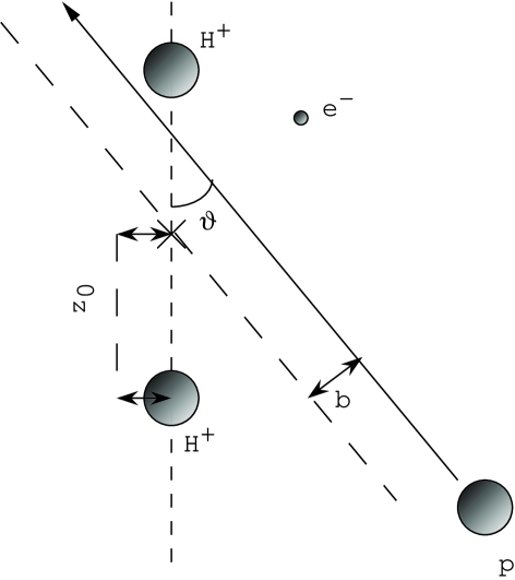
FIG. 2.: Sketch of the geometrical arrangement of the collision. The two $H+$ are the nuclei of the $H^{+}_{2}$ molecule, $p$ is the projectile and $e^{-}$ the electron. $z_{0}$ is half the internuclear distance, $b$ the impact parameter, $\vartheta$ the angle of impact and $d$ the initial distance. For easiness, a coplanar collision is sketched: in the general case the projectile must be rotated out of the plane of an angle $\phi_{rot}$ uniformly chosen within the range ($0,2\pi$).

FIG. 3.: Electron capture cross section $\sigma_{cx}$ versus azimuthal angle $\vartheta$ for different impact velocities. Errors bars are not shown as they are of the same size of the symbols.

FIG. 4.: Anisotropy parameter $A$ versus $v$.

FIG. 5.: (a) Total electron capture cross section $\sigma_{cx}$, averaged over angle $\vartheta$, versus $v$. At $v=2$ are also shown the data taken from ref. [14]: OBK approximation (full circle), B1B approximation (full square), Ba1 approximation (full triangle); see also the text. (b) The same data, but rescaled according Janev [23]: $\sigma_{cx}/n_{eff}^{4}$ versus $v^{2}n_{eff}^{2}$. The squares are the results from the present work, the solid line the fit from ref. [23].

REFERENCES

- [1] J.C. Houver, D. Dowek, C. Richter, and N. Andersen, Phys. Rev. Lett. 68, 162 (1992).
- [2] K.B. MacAdam, L.G. Gray, and R.G. Rolfes, Phys. Rev. A 42, 5269 (1990); T. Wörmann, Z. Roller-Lutz, and H.O. Lutz, Phys. Rev. A 47, R1594 (1993); S.B. Hansen, et al., Phys. Rev. Lett. 71, 1522 (1993); T. Ehrenreich, et al., J. Phys. B: At. Mol. Opt. Phys. 27, 383 (1994).
- [3] C. Richter, et al., J. Phys. B: At. Mol. Opt. Phys. 26, 723 (1993); Z. Roller-Lutz, Y. Wang, K. Finck, and H.O. Lutz, Phys. Rev. A 47, R13 (1993).
- [4] E. Lewartowski and C. Courbin, J. Phys. B: At. Mol. Opt. Phys. 26, 3403 (1993); S. Bradenbrink, et al, J. Phys. B: At. Mol. Opt. Phys. 27, L391 (1994); J. Wang and R.E. Olson, J. Phys. B: At. Mol. Opt. Phys. 27, 3707 (1994).
- [5] D.H. Homan, M.J. Cavagnero, and D.A. Harmin, Phys. Rev. A 50 R1965 (1994).
- [6] A. Dubois, S.E. Nielsen, and J.P. Hanssen, J. Phys. B: At. Mol. Opt. Phys. 26, 705 (1993); Z. Roller-Lutz, Y. Wang, K. Finck, and H.O. Lutz, J. Phys. B: At. Mol. Opt. Phys. 26, 2967 (1993); M.F.V. Lundsgaard, Z. Chen, C.D. Lin, N. Toshima, Phys. Rev. A 51, 1347 (1995).
- [7] M.F.V. Lundsgaard, N. Toshima, Z. Chen, and C.D. Lin, J. Phys. B: At. Mol. Opt. Phys. 27, L611 (1994).
- [8] S. Schippers, Nucl. Instr. Methods Phys. Res. B 98, 177 (1995).
- [9] C.J. Lundy, R.E. Olson, Nucl. Instr. Methods Phys. Res. B 98 (1995) 223; R.E. Olson and R. Hoekstra, ibid 214; I. Fourré and C. Courbin, Z. Phys. D 38, 103 (1996); S. Bradenbrink, H. Reihl, Z. Roller-Lutz, and H.O. Lutz, J. Phys. B: At. Mol. Opt. Phys. 28, L133 (1995); J. Wang, R.E. Olson, K. Cornelius, and K. Tökési, J. Phys. B: At. Mol. Opt. Phys.29, L537 (1996); J.W. Thomsen, et al., Z. Phys. D 37, 133 (1996).
- [10] N.C. Deb, A. Jain, and J.H. McGuire, Phys. Rev. A 38, 3769 (1988).
- [11] Y.D. Wang, J.H. McGuire, and R.D. Rivarola, Phys. Rev. A 40, 3673 (1989).
- [12] S. Cheng, et al., Nucl. Instr. Methods Phys. Res. B 56/57, 78 (1991).
- [13] C. Illesca and A. Riera, J. Phys. B: At. Mol. Opt. Phys. 31, 2777 (1998).
- [14] S.E. Corchs, R.D. Rivarola, J.H. McGuire, and Y.D. Wang, Phys. Rev. A 47, 201 (1993).
- [15] R.A. Abrines and I.C. Percival, Proc. Phys. Soc. 88, 861, 873 (1966); R.E. Olson and A. Salop, Phys. Rev. A 16, 531 (1977).
- [16] D.R. Schultz, C.O. Reinhold, R.E. Olson, and D.G. Seely, Phys. Rev. A 46, 275 (1992).
- [17] A. Salop, J. Phys. B: At. Mol. Phys. 12, 919 (1979); R.E. Olson, Phys. Rev. A 24, 1726 (1981).
- [18] A.E. Wetmore and R.E. Olson, Phys. Rev. A 38, 5563 (1988).
- [19] L. Salasnich and F. Sattin, Phys. Rev. A 51, 4281 (1995); J.S. Cohen, Phys. Rev. A 54, 573 (1996).
- [20] J.S. Cohen, J. Phys. B: At. Mol. Opt. Phys. 18, 1759 (1985).
- [21] L. Salasnich and F. Sattin, J. Phys. B: At. Mol. Opt. Phys. 29, 751 (1996).
- [22] J. Wang and R.E. Olson, Phys. Rev. Lett. 72, 332 (1994).
- [23] R.K. Janev, Phys. Lett. A 160, 67 (1991).