Application of numerical methods to modeling
the stellar wind and interstellar medium interaction

Abstract

Interaction between the stellar wind, including the solar wind, and the interstellar medium has long been the subject of investigation by both astrophysicists and fluid dynamicists. This is, first, due to the possibility of comparison of physical models for such interaction with the measurements performed by Voyager, Pioneer, and Ulysses spacecrafts. On the other hand, a complicated structure of the flow containing several discontinuities makes it a challenging problem for the application of modern numerical methods both in gasdynamic and magnetogasdynamic (MHD) cases.

In the solar wind case, the problem becomes even more complicated, since the charge-exchange processes between ions and neutral particles must be taken into account. The continuum equations are not applicable to the description of the neutral particle motion, for their mean free path is much larger than the characteristic length scale of the problem. In this case, either approximate coupling models or direct Monte-Carlo simulation are required. The spatial nonuniformity of the solar wind and its perturbations and periodicity make the problem three-dimensional and nonstationary. From a mechanical viewpoint the problem represents the interaction of the uniform interstellar medium and the spherically-symmetric (or asymmetric) solar wind flow. We consider various approaches used by different authors to solve this problem numerically.

The presence of the contact surface dividing the two flows rises the question of its stability. We discuss the reasons of such instabilities and parameters which influence it.

The presence of the interstellar magnetic field necessitates solution of the MHD equations for proper analysis of the obtained data. Although the system of governing equations remains hyperbolic in this case, the multivariance of the exact solution to the MHD Riemann problem makes inefficient its application for regular calculations. On the other hand, the solution to the linearized Riemann problem is nonunique. We discuss the possible ways of applying the Roe-type methods and some simplified approaches for numerical solution of the ideal MHD equations. One of the difficulties in the solution of the MHD system is the satisfaction of the magnetic field divergence-free condition. Different ways to solve this task are discussed. If the magnetic field vector in the uniform interstellar medium flow is not parallel to the velocity vector, the problem becomes three-dimensional. Both approximate and exact numerical solutions are considered which were applied in this case.

Far-field numerical boundary conditions play an essential role in astrophysical applications owing to very large length scales usual for these problems. We discuss several approaches that may be useful to solve problems similar to the stellar wind and interstellar medium interaction.

1 INTRODUCTION

The problem of the stellar wind, with the emphasis on the solar wind, interaction with the interstellar medium has long been the topic of interest for astrophysicists and specialists in the field of the solar–terrestrial physics [2], [3], [21], [28], and [69]. In [6], the application of the continuum equations for this problem is systematically discussed. The first qualitative model for the interaction of the solar wind (SW) and the local interstellar medium (LISM) was proposed by E.N. Parker [69]. He assumed the interstellar medium to be a subsonic stream with the Mach number $\it M_{\infty}\ll 1$ (see Fig. 1).

Here HP is a heliopause dividing the SW and the LISM flow. Generally speaking the above assumption is not correct, since the velocity of the interstellar medium is $\it V_{\infty}\sim 20$ km/s and the scattering experiments for the solar radiation show that the temperature $\it T_{\infty}$ of charged particles constituting the LISM is about $\it 10^{4}K$. Taking into account that the number density of charged particles is usually considered to be $\it n_{\infty}\sim 0.1\,{\rm cm}^{-3}$, the LISM flow can most likely be supposed supersonic than subsonic. The supersonic model of the interaction was first proposed in [5]. The important feature of this approach lies in the application of the continuum (Euler gasdynamic) equations only to the charged particles of both counteracting winds. Although the presence of turbulent pulsations of plasma is supposed to be insignificant for the mean flow structure, their influence is realized by a remarkable change of transport coefficients due to the possibility of scattering of charged particles on electromagnetic plasma fluctuations. This results in the substantial decrease of their mean free path compared with that calculated on the basis of the Coulomb collisions. The solar wind consists mainly of electrons and protons with the number density $\it n_{e}\sim 10\,{\rm cm}^{-3}$ and velocity $\it V_{e}\sim 400\hbox{--}500\rm\,km/s$ and is also considered supersonic. The index “$\it e$” corresponds to values measured at $\it 1{\rm AU}=1.5\times 10^{11}\,$km, that is, at the Earth distance from the Sun. Thus, we can consider this problem, from a gasdynamic viewpoint, as a an interaction of the supersonic spherically-symmetric (or asymmetric) source flow of SW with the uniform supersonic LISM flow. This assumption gave rise to a so-called two-shock model. Generally speaking, this model can be easily obtained numerically if one choses as initial data for this interaction the arbitrary jump between the SW and the LISM parameters.

The source flow is essentially a combination of supersonic jet and blunt-body flows which are perfectly well studied and described in classical gas dynamics. The extension to the solar wind and space situation [31], [95] has been validated by numerous spacecraft observations of the plasma environment of several planets. Different flow regimes and shock-wave flow structure for the SW–LISM interaction was discussed in [106].

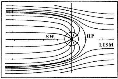
Figure 1: Schematic picture of the SW–LISM interaction [3]

In [7] and [113] the axisymmetric problem of the interaction was considered on the basis of the shock-fitting approach, but due to the limitations of the applied numerical method the authors calculated only the upwind part of the flow. In [55] and [92] the problem of the stellar wind interaction with the interstellar medium was analyzed in the closed region surrounding the star. These numerical results confirmed the scheme [106], but the bullet shape of the internal shock was obtained for a broader range of parameters. The general schematic picture is shown in Fig. 2.

Here TS is the inner shock terminating the solar wind within the heliopause (HP), BS is the bow shock, or the outer shock. TS at a certain point may turn to form the Mach disk (MD). At this triple point the reflected shock (RS) and the slip line (SL) originate.

This picture is similar to that suggested for the SW–comet interaction in [106]. The termination shock configuration is caused by its Mach-type reflection from the symmetry axis.

In [3], [18], [29], [32], [40], [104], and [105] the opinion was stated that the resonance recharge processes between the neutral and the charged particles should strongly influence the flow picture. The description of the neutral particle motion cannot be made on the basis of the continuum approach. For this reason in [8] an approximate method of taking into account this influence was suggested and, later, in [11] a self-consistent model was developed that takes into account the recharge processes. The Monte-Carlo method was used to calculate the trajectories of neutral particles. As was admitted in [104] and confirmed by [8] and [11], the charge-exchange effect effectively diminishes the Mach number of the LISM flow. This justifies development of alternative subsonic models of the interaction [48].

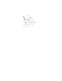
Figure 2: General scheme of supersonic interaction

Of great importance are also nonstationary problems associated with the variable solar activity. In [15], [75], and [97] the problem was investigated of the time-dependent SW perturbation influence on the whole flow structure. The nonstationary picture of the flow and the termination shock response to the 11-year variation of the solar wind were studied in [17], [47], and [76].

T. Matsuda et al. [55] discussed the instabilities of the contact discontinuity dividing the SW and the LISM flow. These instabilities originated in its lateral region and near the stagnation point of the flow. Unstable solutions were obtained in the parameter range which was not exactly suitable for the solar wind and the local interstellar medium flow and, therefore, were disputed in [96]. Recently in [52] a hydrodynamic instability of the heliopause driven by plasma–neutral charge-exchange processes was discussed.

According to the solar minimum observations by the Ulysses spacecraft, the solar wind properties depend on helioaltitude. The solar wind in this case is no longer spherically-symmetric (see also [99]). In [71] a 3D problem of the interaction was used and obtained results were compared with those for the isotropic solar wind.

The influence of the interstellar magnetic field can be important in the regions, for which the magnetic pressure is comparable by its value with the dynamic pressure of the flow. Magnetic field causes an increase of the maximum speed of small perturbations in the LISM flow, thus leading to the decrease of its effective Mach number [33], [34]. The ordinary Mach number of the LISM is often assumed to be $\it M_{\infty}=2$. At the same time the magnitude of the LISM magnetic field, although not known very well, is estimated within $\it 7\times 10^{-7}$ and $\it 3\times 10^{-6}$ Gauss [3]. This means, as will be shown later, that the magnetic pressure can exceed the value of the thermal pressure and is the reason of including magnetic field into consideration. Its influence can be especially effective when the charge-exchange processes are included, since both this effects lead to the decrease of the effective Mach number. This means that the LISM flow can become subsonic and the bow shock can disappear (see also [33] and [104]). The stellar wind–interstellar medium interaction with taking into account magnetic field was first studied in [59], although some of the results seem to be misinterpreted (see [12]). In the latter paper the problem was investigated by the shock-fitting method only in the upwind part of the flow due to the limitations of the numerical scheme. In [80] the solution was presented of the axisymmetric problem (the LISM magnetic field strength vector was assumed to be parallel to its velocity vector) of the SW–LISM interaction in the closed region surrounding the star. In [34] the shape of the heliopause was studied on the basis of the Newtonian approach in the 3D case of the arbitrary angle between the LISM magnetic field and velocity vectors. The authors found this shape approximately by equating the values of the total pressure on the both sides of the heliopause. In [81] this problem was first examined numerically.

The complicated pattern of the flow containing a number of interacting shocks, enhanced by various physical phenomena, makes it a challenging problem for the application of modern numerical methods invented for pure gasdynamic and magnetogasdynamic application. Numerical solution of this problem is often associated with the solution of such accompanying problems as non-reflecting boundary conditions, numerical implementation of the condition of the magnetic charge absence, etc. These problems are of general importance for the young, but quickly developing, field called computational fluid dynamics. In Section 2 of this review we present the mathematical statement of the problem, write out the system of governing equations and boundary conditions. The choice of initial conditions for the magnetogasdynamic (MHD) interaction is discussed. In Section 3 we discuss stationary solutions of the gasdynamic problem on the basis of shock-fitting and shock-capturing methods. In Section 4 different approaches are discussed which take into account the charge-exchange processes. In Section 5 we describe instabilities originating under certain circumstances in this problem and the reasons causing them. In Section 6 nonstationary solutions are considered resulting from the solar wind disturbances and its periodicity. In Section 7 we briefly discuss the effects of the solar wind spatial asymmetry. And, finally, Section 8 deals with numerical modeling of the solar wind interaction with the magnetized interstellar medium.

2 Mathematical statement of the problem

To make the paper more concise, we write out in this section the mathematical statement of the problem based on the MHD equations. The Euler gasdynamic equations can be easily obtained from the former one by omitting the terms containing the magnetic field strength and the equations describing the behavior of its components.

2.1 The system of governing equations

The system of governing equations for a MHD flow of an ideal, infinitely conducting, perfect plasma in the Cartesian coordinate system $\it x$, $\it y$, $\it z$, shown in Fig. 2 ($\it y$-axis is perpendicular to the picture plane), can be written as follows (one fluid approximation):

$${\partial{\bf U}\over\partial t}+{\partial{\bf E}\over\partial x}+{\partial{\bf F}\over\partial y}+{\partial{\bf G}\over\partial z}+{\bf H}=\mathchar 1584\relax\,,$$ (1)

where

$$\it\displaystyle{\bf U}=\left[\begin{array}[]{c}\rho\\ \rho u\\ \rho v\\ \rho w\\ e\\ B_{x}\\ B_{y}\\ B_{z}\\ \end{array}\right],\quad{\bf E}=\left[\begin{array}[]{c}\rho u\\ \displaystyle\rho u^{2}+p_{0}-{B_{x}^{2}\over 4\pi}\\ \kern 2.0pt\cr\displaystyle\rho uv-{B_{x}B_{y}\over 4\pi}\\ \kern 2.0pt\cr\displaystyle\rho uw-{B_{x}B_{z}\over 4\pi}\\ \kern 2.0pt\cr\displaystyle(e+p_{0})u-{B_{x}\over\displaystyle 4\pi}({\bf v}\cdot{\bf B})\\ 0\\ uB_{y}-vB_{x}\\ uB_{z}-wB_{x}\\ \end{array}\right],\,$$

$$\it\displaystyle{\bf F}=\left[\begin{array}[]{c}\rho v\\ \displaystyle\rho uv-{B_{x}B_{y}\over 4\pi}\\ \displaystyle\rho v^{2}+p_{0}-{B_{y}^{2}\over 4\pi}\\ \kern 2.0pt\cr\displaystyle\rho vw-{B_{y}B_{z}\over 4\pi}\\ \kern 2.0pt\cr\displaystyle(e+p_{0})w-{B_{y}\over 4\pi}({\bf v}\cdot{\bf B)}\\ \kern 2.0pt\cr vB_{x}-uB_{y}\\ 0\\ vB_{z}-wB_{y}\\ \end{array}\right],\,$$

$$\it\displaystyle{\bf G}=\left[\begin{array}[]{c}\rho w\\ \displaystyle\rho uw-{B_{x}B_{z}\over 4\pi}\\ \kern 2.0pt\cr\displaystyle\rho vw-{B_{y}B_{z}\over 4\pi}\\ \displaystyle\rho w^{2}+p_{0}-{B_{z}^{2}\over 4\pi}\\ \kern 2.0pt\cr\displaystyle(e+p_{0})w-{B_{z}\over 4\pi}({\bf v}\cdot{\bf B)}\\ wB_{x}-uB_{z}\\ wB_{y}-vB_{z}\\ 0\\ \end{array}\right]$$

In system (1) $\it\rho$, $\it u$, $\it v$, $\it w$, $\it B_{x}$, $\it B_{y}$, and $\it B_{z}$ are the density and the components of the velocity $\it\bf v$ and of the magnetic field strength vector $\it\bf B$. We introduced here also the total pressure $\it p_{0}=p+{\bf B}^{2}\!/8\pi$ ($\it p$ is the thermal pressure) and the total energy per unit volume

$$\it\it e={p\over\gamma-1}+{\rho(u^{2}+v^{2}+w^{2})\over 2}+{{\bf B}^{2}\over 8\pi}\,,$$

where $\it\gamma=5/3$ is the specific heat ratio corresponding to the fully ionized plasma. The quantities of density, pressure, velocity, and magnetic field strength are normalized, respectively, by $\it\rho_{\infty}$, $\it\rho_{\infty}V^{2}_{\infty}$, $\it V_{\infty}$, and $\it V_{\infty}\sqrt{\rho_{\infty}}$, where the index “$\it\infty$” marks the values in the uniform LISM flow. Time and the linear dimension are respectively related to $\it L/V_{\infty}$ and $\it L$, where $\it L$ is equal to $\it 1\,{\rm AU}$. The above formulation implies that molecular and magnetic viscosities, heat conductivity, and anomalous transport effects are neglected. The source term $\it{\bf H}$ can be both of physical and of geometrical origin and will be specified separately for each problem. For example, if the flow is axisymmetric system (1) can be rewritten in the plane coordinate system $\it x,\,z$ as follows:

$${\partial{\bf U}\over\partial t}+{\partial{\bf E}\over\partial x}+{\partial{\bf G}\over\partial z}+{\bf H}=\mathchar 1584\relax\,,$$ (5)

where

$$\it\displaystyle{\bf U}=\left[\begin{array}[]{c}\rho\\ \rho u\\ \rho w\\ e\cr B_{x}\\ B_{z}\\ \end{array}\right],\quad{\bf H}={1\over x}\left[\begin{array}[]{c}\rho u\\ \displaystyle\rho u^{2}-{B_{x}^{2}\over 4\pi}\\ \kern 2.0pt\cr\displaystyle\rho uw-{B_{x}B_{z}\over 4\pi}\\ \kern 2.0pt\cr\displaystyle(e+p_{0})u-{B_{x}\over 4\pi}({\bf v}\cdot{\bf B})\\ 0\\ uB_{z}-wB_{x}\\ \end{array}\right],$$

$$\it\displaystyle{\bf E}=\left[\begin{array}[]{c}\rho u\\ \displaystyle\rho u^{2}+p_{0}-{B_{x}^{2}\over 4\pi}\\ \kern 2.0pt\cr\displaystyle\rho uw-{B_{x}B_{z}\over 4\pi}\\ \kern 2.0pt\cr\displaystyle(e+p_{0})u-{B_{x}\over\displaystyle 4\pi}({\bf v}\cdot{\bf B})\\ 0\\ uB_{z}-wB_{x}\\ \end{array}\right],\,$$

$$\it\displaystyle{\bf G}=\left[\begin{array}[]{c}\rho w\\ \displaystyle\rho uw-{B_{x}B_{y}\over 4\pi}\\ \displaystyle\rho w^{2}+p_{0}-{B_{z}^{2}\over 4\pi}\\ \displaystyle(e+p_{0})w-{B_{z}\over 4\pi}({\bf v}\cdot{\bf B)}\\ wB_{x}-uB_{z}\\ 0\\ \end{array}\right]$$

This system is valid in the half-plane $\it x0z$ and can be obtained from (1) in the assumption of cylindrical symmetry. Its another form is

$${\partial{x\bf U}\over\partial t}+{\partial{x\bf E}\over\partial x}+{\partial{x\bf G}\over\partial z}+{\tilde{\bf H}}=\mathchar 1584\relax\,,$$ (9)

where

$$\it\it{\tilde{\bf H}}=[0,{-p_{0}},\,0,\,0,\,0,\,0]^{\rm T}$$

Though both presentations of governing equations are mathematically equivalent, for numerical reasons it is often more convenient to use the former one, since it is supposed to give more stable results in the vicinity of the geometrical singularity $\it x=0$. The Euler gasdynamic equations can be obtained in different forms from systems (1) and (2) by assuming $\it{\bf B}\equiv\mathchar 30256\relax$.

2.2 Initial and boundary conditions

Calculations are usually performed in the computational region between the inner and the outer spherical surface (circular in the axisymmetric case). The flow from the Sun is supposed to be supersonic at the termination shock distance. For this reason we specify all parameter values at the inner boundary sphere. The uniform LISM flow is also supersonic and we can specify the parameter values at the inflow side of the outer boundary. The treatment of outflow boundary can be more complicated. In [96] all parameters were extrapolated with the zeroth order along the fluid particle trajectory. This approach cannot be expected suitable for deeply subsonic outflow boundary. Another approach was proposed in [92]. This method is based on introducing imaginary cells next to the boundary. These cells are filled with the LISM gas at infinity. To find the flux through the outer boundary the Riemann problem is solved between the imaginary and the adjacent cell values. At the boundary segments with the subsonic–supersonic transition the rarefaction wave relations are used. This results in the following interpretation (see [75] and [78]) of the method initially developed for a purely gasdynamic case and makes possible its extension to MHD problems [80].

Consider the method based on the two strictly nonreflecting conditions: the well-known extrapolation condition for a supersonic exit that provides a characteristically compatible approximation of the equations on the boundary and the procedure [75], [78], developed earlier for gasdynamic flows.

The idea of application of the relations in the rarefaction wave for the realization of the far-field boundary conditions lies in the artificial locating of the sonic point on the exit boundary. If the flow is supersonic at infinity such a procedure gives reasonable results and allows one to perform calculations in the cases for which other known approaches fail. The interpretation of our method is the following. Assume that parameters inside the chosen computational region fully define the flow behavior outside the boundary. In the case of subsonic exit the only possible elementary Riemann problem configuration for the above system is a rarefaction wave whose fan covers the boundary. In this case, if the self-similar variable value is known, we can locally continue the internal field to the boundary. That is why, an additional condition is that the flow velocity attains the sonic value there.

Consider the hyperbolic system for the vector $\it\bf U$ of unknown variables in the vicinity of the boundary (the right one for definiteness) in the form

$${\partial{\bf U}\over\partial t}+A{\partial{\bf U}\over\partial x}=\mathchar 1584\relax\,,$$ (10)

where $\it{\bf U}={\bf U}(x,t)$, and $\it x$ is the variable in the direction normal to the boundary $\it\mathchar 0\relax$, $\it t$ is time, and $\it A({\bf U})$ is the coefficient matrix with a complete set of eigenvectors and only real eigenvalues. We seek the solution in the form of a simple wave $\it{\bf U}={\bf U}(x,t)={\bf U}(\xi)$, where $\it\xi={x\over t}$. By substituting this representation into Eq. (4), we obtain

$$(A-\lambda I){\bf U}_{\xi}={\bf 0},\quad\lambda=\xi\,,$$ (11)

where $\it I$ is the identity matrix. Owing to Eq. (5), the vector $\it{\bf U}_{\xi}$ is the eigenvector of A for the eigenvalue $\it\lambda=\xi$. This means that we need to solve the following system of ordinary differential equations supplemented by the nondifference relation:

$${\bf U}_{\xi}=d({\bf U},\lambda){\bf r}{(\bf U},\lambda)\,,\quad\lambda({\bf U})=\xi\,,$$ (12)

where $\it\bf r$ is the right eigenvector (the vector-column) of $\it A$ defined up to the scalar multiplier $\it d$. The eigenvalue in the rarefaction wave varies like $\it\lambda({\bf U})=\xi$. This condition completes the system for determining $\it{\bf U}$ and $\it d$. While realizing this boundary condition we must integrate Eq. (6) over $\it\xi$ from $\it\xi_{0}=\lambda({\bf U}_{0})$, where $\it{\bf U}_{0}$ represents the initial subsonic parameters inside the region, to $\it\xi=\xi_{\mathchar 0\relax}=0$, that is, to the sonic point. Consider this approach, first, for pure gas dynamics. Let us choose the vector of unknowns in Eq. (4) in the form $\it{\bf U}=(\rho,u,v,w,a)^{T}$, where $\it\rho$ is the density, $\it u$ is the velocity vector component normal to $\it\mathchar 0\relax$, $\it v$ and $\it w$ are its tangential components, and $\it a$ is the speed of sound. The minimum eigenvalue in this case is $\it\lambda=u-a$ and the related eigenvector is

$${\bf r}=\left[1,\ -{a\over\rho},\ 0,\ 0,\ {(\gamma-1)a\over 2\rho}\right]^{\rm T}\,,$$ (13)

where $\it\gamma$ is the adiabatic index. System (6) in this case acquires the form

$$\it\displaystyle\rho_{\xi}=d,\ u_{\xi}=-{ad\over\rho},\ v_{\xi}=0,\ w_{\xi}=0,$$

(14)

$$\it\displaystyle a_{\xi}={(\gamma-1)ad\over 2\rho},\ u-a=\xi.$$

This system can be exactly integrated, as its invariants are

$$\left({p\over\rho^{\gamma}}\right)_{\xi}=0,\ \left(u+{2a\over\gamma-1}\right)_{\xi}=0,\ v_{\xi}=0,\ w_{\xi}=0.$$ (15)

Thus, we obtain

$$\it\displaystyle a_{\mathchar 0\relax}={\gamma-1\over\gamma+1}\left(u_{0}+{2\over\gamma-1}a_{0}\right),\ u_{\mathchar 0\relax}=a_{\mathchar 0\relax},\ v_{\mathchar 0\relax}=v_{0}\,,$$

(16)

$$\it\displaystyle w_{\mathchar 0\relax}=w_{0},\ \rho_{\mathchar 0\relax}=\rho_{0}\left(a_{\mathchar 0\relax}\over a_{0}\right)^{2\over\gamma-1}$$

The index “0” indicates the values belonging to the inner region. On the discreet mesh this means that they are taken from the center (or from the left side) of the cell adjacent to the boundary. Equations (10) must be supplemented by the condition at the supersonic exit if $\it(u/a)_{0}\geq 1$: $\it{\bf U}_{\mathchar 0\relax}={\bf U}_{0}$.

These conditions are mutually consistent and coincide for $\it u_{0}=a_{0}$. Note that in this case we did not need the explicit expression for $\it d$ which can be easily found from the second and the fifth equations in (8). Besides the exact derivation based on the relations in the rarefaction wave, we give here the approximate relations keeping in mind such systems for which no exact expressions of this kind can be written out. For this purpose we first exclude $\it d$ by substituting the first equation from (8) into the other ones. Then we obtain

$$\it\displaystyle u_{\xi}=-{a\rho_{\xi}\over\rho},\ \ v_{\xi}=0,\ \ w_{\xi}=0,$$

(17)

$$\it\displaystyle a_{\xi}={(\gamma-1)a\rho_{\xi}\over 2\rho},\ \ u-a=\xi$$

Now, approximating Eqs. (11) by finite differences we arrive at the following relations:

$$\it\displaystyle a_{\mathchar 0\relax}={\gamma-1\over\gamma+1}\left(u_{0}+{2\over\gamma-1}a_{0}\right),\ u_{\mathchar 0\relax}=a_{\mathchar 0\relax},\ v_{\mathchar 0\relax}=v_{0}\,,$$

(18)

$$\it\displaystyle w_{\mathchar 0\relax}=w_{0},\ \rho_{\mathchar 0\relax}=\left[1+{2\over\gamma-1}\left({a_{\mathchar 0\relax}\over a_{0}}-1\right)\right].$$

In this approximation solution (12) differs from (10) only in the entropy invariant and represents its linearization.

Now we proceed to the MHD equations. Let us choose the unknown vector in Eq. (4) in the form

$${\bf U}=[\rho,\ u,\ v,\ w,\ a,\ B_{x},\ B_{y},\ B_{z}]^{\rm T}.$$ (19)

where, in addition to the purely gasdynamic case, the components appear of the magnetic field strength vector normal ($\it B_{x}$) and tangential ($\it B_{y}$ and $\it B_{z}$) to $\it\mathchar 0\relax$. The minimum eigenvalue in this case is $\it\lambda=u-a_{f}$, where $\it a_{f}$ is the largest of the two magnetosonic speeds $\it a_{f}$ and $\it a_{s}$ ($\it a_{f}>a>a_{s}$):

$$\it\displaystyle a_{f,s}=\frac{1}{2}\Biggl{[}\left(a^{2}+{|{\bf B}|^{2}\over 4\pi\rho}+{a|B_{x}|\over\sqrt{\pi\rho}}\right)^{1/2}$$

(20)

$$\it\displaystyle\pm\left(a^{2}+{|{\bf B}|^{2}\over 4\pi\rho}-{a|B_{x}|\over\sqrt{\pi\rho}}\right)^{1/2}\Biggr{]},\ |{\bf B}|^{2}=B_{x}^{2}+B_{y}^{2}+B_{z}^{2}$$

The eigenvector corresponding to this eigenvalue is

$$\it\displaystyle{\bf r}=\left[1,\,-{a_{f}\over\rho},\,\alpha B_{y},\,\alpha B_{z},\,{(\gamma-1)a\over 2\rho},\,0,\,\beta B_{y},\,\beta B_{z}\right]^{\rm T},\,$$

(21)

$$\it\displaystyle\alpha={aa_{s}\over 2\rho\sqrt{\pi\rho}(a^{2}-a_{s}^{2})},\,\beta={a^{2}\over\rho(a^{2}-a^{2}_{s})}\,$$

In this case system (6) acquires the form

$$\it\displaystyle\rho_{\xi}=d,\,u_{\xi}=-{a_{f}d\over\rho},\,v_{\xi}=\alpha B_{y}d,\,w_{\xi}=\alpha B_{x}d\,,$$

$$\it\displaystyle a_{\xi}={(\gamma-1)ad\over 2\rho},\,(B_{x})_{\xi}=0,\,(B_{y})_{\xi}=\beta B_{y}d\,,$$ (22)

$$\it\displaystyle(B_{z})_{\xi}=\beta B_{y}d,\,u-a_{f}=\xi\,$$

Now in system (16) we substitute the equation for $\it a$ by the equation for $\it a_{f}$, which can be easily obtained from Eq. (14) by direct differencing with respect to $\it\xi$ and by using Eqs. (16):

$$(a_{f})_{\xi}={\vartheta d\over\rho},\ \vartheta=\rho{\bf r}{\partial a_{f}\over\partial{\bf U}}\,.$$ (23)

It can be shown in this connection that for any admissible values of functions we have $\it\vartheta+a_{f}\geq 0$.

Then, by passing from $\it d$ to $\it\rho_{\xi}$, we obtain the reduced system of equations that can be approximated similarly to Eq. (11)

$$\it\displaystyle(a_{f})_{\mathchar 0\relax}=\left({u\vartheta+a^{2}_{f}\over\vartheta+a_{f}}\right)_{0},\,\rho_{\mathchar 0\relax}=\rho_{0}\left(1+{u-a_{f}\over\vartheta+a_{f}}\right)_{0}\,,$$

$$\it\displaystyle u_{\mathchar 0\relax}=(a_{f})_{\mathchar 0\relax},\,v_{\mathchar 0\relax}=v_{0}+(\alpha B_{y})_{0}(\rho_{\mathchar 0\relax}-\rho_{0})\,,$$

$$\it\displaystyle w_{\mathchar 0\relax}=w_{0}+(\alpha B_{z})_{0}(\rho_{\mathchar 0\relax}-\rho_{0}),\,(B_{x})_{\mathchar 0\relax}=(B_{x})_{0}\,,$$ (24)

$$\it\displaystyle(B_{y})_{\mathchar 0\relax}=(B_{y})_{0}[1+\beta_{0}(\rho_{\mathchar 0\relax}-\rho_{0})]\,,$$

$$\it\displaystyle(B_{z})_{\mathchar 0\relax}=(B_{z})_{0}[1+\beta_{0}(\rho_{\mathchar 0\relax}-\rho_{0})]\,,$$

$$\it\displaystyle(a)_{\mathchar 0\relax}=(a)_{0}+(\gamma-1)(a/2\rho)_{0}(\rho_{\mathchar 0\relax}-\rho_{0})\,$$

Note that in contrast to the purely gasdynamic case the velocity components tangential to the boundary, generally speaking, are different from their internal values in the presence of the magnetic field.

The case of the triple degeneration of eigenvalues ($\it B_{y}^{2}+B_{z}^{2}=0$ and $\it a^{2}\to B_{x}^{2}/4\pi\rho$), when $\it\vartheta+a_{f}\to\infty$, can be easily avoided by assuming $\it B_{y}^{2}+B_{z}^{2}=\varepsilon$, where $\it\varepsilon$ is a small positive number.

The approach described above turned out to give stable results in contrast to the attempts of a straight application of the well-known non-reflecting boundary conditions, say, [102]. It is worth mentioning in this connection that a comprehensive review (more than 200 references) of various versions and modifications of non-reflecting boundary conditions can be found in [43] and [44] (see also [37] and [102]).

As initial values the jump can be chosen between the SW and the LISM parameters at a fixed distance $\it R_{\rm f}$ from the Sun smaller than the TS stand-off distance. For $\it R<R_{\rm f}$ the SW parameter distribution is specified. The magnetic field pressure in this region is supposed to be negligibly small comparing with the SW hydrodynamic pressure, thus $\it{\bf B}_{e}={\bf 0}$. For $\it R>R_{\rm f}$ the uniform distribution of the LISM pressure and density is assumed. If we solve an MHD problem, that is, the LISM flow is magnetized, it is wise to specify a magnetic field strength distribution satisfying the divergence-free condition. For this reason the magnetic and the velocity field in the LISM and in the SW flow are initially joined in the computational region so that $\it{\bf B}$ conserves a constant angle with $\it{\bf v}$ and $\it\mathop{\rm div}\nolimits{\bf B}=0$. This is done by assuming for $\it R>R_{\rm f}$

$$\it\displaystyle U=-V_{\infty}\left[1-\left({R_{\rm f}\over R}\right)^{3}\right]\cos\theta$$

$$\it\displaystyle V=0$$ (25)

$$\it\displaystyle W=V_{\infty}\left[1+{1\over 2}\left({R_{\rm f}\over R}\right)^{3}\right]\sin\theta\,$$

Here $\it U$, $\it V$, and $\it W$ represent the spherical components of the velocity vector in the directions $\it R$, $\it\phi$, and $\it\theta$, respectively. This distribution corresponds to an incompressible fluid flow velocity distribution over a sphere, directed along the $\it z$-axis ($\it\theta$-axis). The magnetic field is initialized in the same way, except that the field configuration is rotated about the $\it y$-axis so that the magnetic field vector is tilted with respect to the velocity vector by the desired angle.

If neutral particles are to be taken into account, we must specify their number density and velocity at the inflow.

3 Stationary gasdynamic calculations

A gasdynamic model for the SW interaction with the supersonic interstellar wind was first suggested in [7]. A cylindrical formulation was adopted which corresponds to a uniform LISM flow and a spherically-symmetric SW. The calculations were performed on the basis of a simplified thin-layer approximation. The solar wind was assumed to be decelerated mainly in the process of its interaction with the charged component, or plasma component, of the LISM. With the latter assumption calculations can also be made without simplifications using the Euler gasdynamic equations. Both shock-fitting and shock-capturing approaches can be found in publications and we describe them briefly in the following subsections.

3.1 Shock-fitting methods

Taking into account the adopted two-shock model with the contact discontinuity between the shocks, one can easily use shock-fitting methods in the upwind part of the interaction region. The idea of this approach lies in the subdivision of the computational region into subregions of smooth flow. In these smooth subregions any numerical scheme of sufficient order of accuracy can be used. Derivatives in this approach must never be approximated by finite differences across discontinuities. The latter are traced as boundary lines. Proper jump relations are used to determine the change of parameters across these boundaries and their new position in the course of time. This approach is very economical, since 1) you need not perform calculations in the regions of the uniform LISM and the spherically-symmetric SW, which are known beforehand, thus reducing the size of the computational domain and 2) you can avoid spurious oscillations around discontinuities inherent in application of shock-capturing methods. For this reason one can use linear high-order of accuracy numerical schemes not worrying about high non-oscillatory resolution of discontinuities. In the shock-fitting method their position and intensity are determined exactly. Certain difficulties originate if two or more discontinuities are interacting with each other. In this case, in principle, one can still use a shock-fitting approach using exact solutions for the problems of a discontinuity interaction. The algorithm, however, can become rather complicated (see [60], [61], [62], and [64]). In the shock-fitting approach a quasi-linear form of the system of governing equations is usually chosen rather than a conservation-law form.

On the basis of the shock-fitting approach the problem under consideration was first solved in [7] by the Babenko–Rusanov implicit scheme [4]. Due to the limitations of the numerical approach only upwind part of the interaction was calculated. A polar coordinate system $\it R,\,\theta$ was used and calculations were performed in the region restricted by the ray $\it\theta=\theta_{\rm max}$ at which the velocity normal to this boundary remained supersonic. The system of linear algebraic equations on the computational grid was solved together with the Rankine–Hugoniot conservation relations and the relations on the contact discontinuity. The computational region was located between the termination and the bow shock. The steady-state solution was obtained as $\it t\to\infty$ with the boundary conditions independent of time.

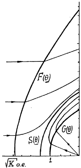
Figure 3: Self-similar picture of shock wave position [7]

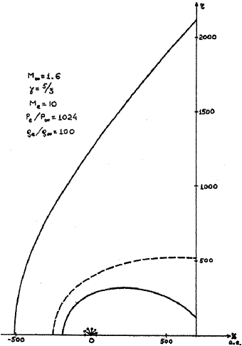
Figure 4: Discontinuity pattern: shock-fitting approach [113]

A physicist usually seeks dimensionless similarity parameters of the problem. For the considered problem they are represented by the Mach numbers $\it M_{e}$ and $\it M_{\infty}$ of the SW and the LISM flow, respectively, the ratios of their dynamic pressures $\it K=n_{e}V_{e}^{2}/n_{\infty}V_{\infty}^{2}$ and stagnation temperatures $\it\chi=T_{e0}/T_{\infty 0}$. The specific heat ratio $\it\gamma$ is usually adopted to be equal to 5/3 which corresponds to the fully ionized plasma. If neutral particles are not taken into account, the flow from the inner side of TS becomes hypersonic and, therefore, the results are only weakly dependent on the choice of $\it M_{e}$ taken at 1 AU. Though results formally depend on $\it\chi$ (say, for $\it\chi=1$ the density jump over CD is absent) an analysis of conservation relations on the discontinuities in the upwind part of the interaction region make us conclude that they can be recalculated using results for one particular value of $\it\chi$. As $\it K$ is the similarity parameter (see [5] and [7]), for the hypersonic solar wind and $\it K>1$ the results are independent of $\it K$ if the distances are measured in units of $\it 1{\rm AU}\times\sqrt{K}$. In Fig. 3, the shapes of the outer (F) and of the inner (G) shock wave, the contact surface (S) and some streamlines are presented for the case $\it M_{\infty}=2$.

In [113] a new shock-fitting numerical algorithm was described and applied to the problem under consideration that provided results with such a high accuracy that in the upwind part of the interaction it may represent a testing benchmark for all newly developed methods. This method is based on the composite explicit-implicit finite-difference scheme [86]. The well-known explicit Lax–Wendroff and the implicit Babenko scheme [4] represent its constituent parts. The algorithm is organized in such a way that depending on the CFL number value either explicit or implicit approximation is used. This approach makes the proposed method more economical than a purely implicit scheme. Among the schemes based on this approach we can also mention [53] and [74]. The latter method is the extension of MacCormack’s explicit-implicit scheme for the steady Euler equations hyperbolic with respect to one of the space coordinates. A steady-state solution of the SW–LISM interaction was obtained in [113] by a quasi-marching method in which nonstationary problem was solved for $\it t\to\infty$ for each radial ray. Such an approach also allowed to save a computational time comparing with a direct solution of the nonstationary system. One of the computational results is shown in Fig 4.

One must admit here that, in contrast to the results from [7], calculations were performed for a rather long distance in the downwind direction, actually until the flow along the $\it z$-axis shown in Fig. 4 remained supersonic. This resulted in a considerable unjustifiable elongation of the termination shock, as will be seen from the subsequent subsection. The discrepancy between the results is caused by the limitation of the quasi-marching approach that cannot take into account the Mach-type reflection of the inner shock from the symmetry axis. Nevertheless, the results are without any doubt quite reliable up to a certain distance in the wake region. No need to mention that the time necessary for obtaining the steady-state solution in this case is considerably less than that in the case of applying shock-capturing methods.

3.2 Shock-capturing methods

In shock-capturing methods we calculate finite differences across discontinuities. This may cause spurious oscillations of the solution if non-monotone numerical schemes are used. On the other hand, all linear schemes of the order of accuracy higher than one are non-monotone [38]. For this reason one or another artificial viscosity must be used [85] or nonlinear numerical schemes ought to be applied. It is not our task to give a review of high-resolution TVD (total variation diminishing) schemes in this paper (see [42] and [112] for a regular mathematical background). Although both finite-difference and finite-volume methods can be equivalently applied in the latter schemes, we shall dwell mainly on the finite-volume formulation and monotonic upstream schemes for conservation laws (MUSCL) approach, since they are more descriptive.

To solve axisymmetric system (2), let us introduce a polar mesh

$$\it\displaystyle f^{k}_{l,n}=f(R_{l},\theta_{n},t^{k})\,,\quad t^{k}=k\mathchar 1\relax t\,;$$

$$\it\displaystyle R_{l}=R_{\rm min}+(l-1)\mathchar 1\relax R,\quad l=1,2,\ldots,L;$$

$$\it\displaystyle\theta_{n}=(n-2.5)\mathchar 1\relax\theta,\quad n=1,2,\ldots,N;$$ (26)

$$\it\displaystyle\mathchar 1\relax R=(R_{\rm max}-R_{\rm min})/(L-1),$$

$$\it\displaystyle\mathchar 1\relax\theta=\pi/(N-4)$$

with the center in the star. Then for each cell system (2) in the finite-volume formulation can be rewritten as follows:

$$\it\displaystyle R_{l}\,\mathchar 1\relax R\,\mathchar 1\relax\theta\,{{\bf U}_{l,n}^{k+1}-{\bf U}_{l,n}^{k}\over\mathchar 1\relax t}+{}$$

$$\it\displaystyle(R_{l+1/2}\bar{\bf E}_{l+1/2,n}+R_{l-1/2}\bar{\bf E}_{l-1/2,n})\,\mathchar 1\relax\theta+{}$$ (27)

$$\it\displaystyle(\bar{\bf E}_{l,n+1/2}+\bar{\bf E}_{l,n-1/2})\,\mathchar 1\relax R+R_{l}\,\mathchar 1\relax R\,\mathchar 1\relax\theta\,{\bf H}_{l,n}=0.$$

Here $\it\bar{\bf E}$ is the flux normal to the boundary, defined as:

$$\bar{\bf E}=n_{1}{\bf E}+n_{2}{\bf G},$$ (28)

where $\it{\bf n}=(n_{1},n_{2})$ is a unit outward vector normal to the cell surface.

Equation (21) has a time-discretized conservation-law form for an individual computational cell. Various numerical schemes are specified by the method chosen to calculate the numerical flux $\it\bar{\bf E}$ through the cell boundary surfaces. In [96] the two-step Lax–Wendroff scheme is used with the second order of accuracy. As usual for such schemes, an additional smoothing must be introduced to remove high-frequency oscillations and overshoots and undershoots originating near smeared shocks owing to the non-monotonicity of the scheme. Another possible flux calculation formulas which also include artificial viscosity were applied in [70]. It is based on the ZEUS fractional step code [98]. All methods using artificial viscosity for oscillation damping contain an empirical viscosity coefficient which must be adjusted in a way suitable for any particular problem. The compromise is between the effective monotonization of the solution and its deterioration. Nonlinear high-resolution numerical schemes are free from this drawback.

To attain the second order of accuracy in space, a piecewise-linear distribution of parameters inside computational cells can be adopted [112]. One can use the simplest “minmod” reconstruction procedure

$$\it\displaystyle{\bf U}^{R}_{l+1/2}={\bf U}^{k}_{l+1}-{\frac{1}{2}}\mathop{\rm min\,mod}\nolimits(\mathchar 1\relax{\bf U}^{k}_{l+1/2},\mathchar 1\relax{\bf U}^{k}_{l+3/2})\,,$$ (29)

$$\it\displaystyle{\bf U}^{L}_{l+1/2}={\bf U}^{k}_{l}+{\frac{1}{2}}\mathop{\rm min\,mod}\nolimits(\mathchar 1\relax{\bf U}^{k}_{l-1/2},\mathchar 1\relax{\bf U}^{k}_{l+1/2})\,,$$ (30)

$$\it\displaystyle\mathop{\rm min\,mod}\nolimits(x,y)=\mathop{\rm sgn}\nolimits(x)\,\max\{0,\min[|x|,y\mathop{\rm sgn}\nolimits(x)]\}\,,$$

where $\it\mathchar 1\relax{\bf U}^{k}_{l+1/2}={\bf U}^{k}_{l+1}-{\bf U}^{k}_{l}$, and $\it{\bf U}^{R}_{l+1/2}$ and $\it{\bf U}^{L}_{l+1/2}$ defined by Eqs. (23)–(24) represent parameter values on the right and on the left side of the cell surface with the index “$\it l+1/2$”. The index “$\it n$” is omitted in these formulas. The reconstruction procedure in the angular direction is similar. To attain better resolution of the contact discontinuity, one can use more compressive slope limiting procedure for the density, e. g.,

$$\it\displaystyle\rho^{R}_{l+1/2}=\rho^{k}_{l+1}-\mathop{\rm min\,mod}\nolimits(\mathchar 1\relax\rho^{k}_{l+1/2},\mathchar 1\relax\rho^{k}_{l+3/2},{\tilde{\mathchar 1\relax}})\,,$$ (31)

$$\it\displaystyle\rho^{L}_{l+1/2}=\rho^{k}_{l}+\mathop{\rm min\,mod}\nolimits(\mathchar 1\relax\rho^{k}_{l-1/2},\mathchar 1\relax\rho^{k}_{l+1/2},{\tilde{\tilde{\mathchar 1\relax}}})\,,$$ (32)

$$\it\displaystyle{\tilde{\mathchar 1\relax}}=0.25(\mathchar 1\relax\rho^{k}_{l+1/2}+\mathchar 1\relax\rho^{k}_{l+3/2})\,,$$

$$\it\displaystyle{\tilde{\tilde{\mathchar 1\relax}}}=0.25(\mathchar 1\relax\rho^{k}_{l-1/2}+\mathchar 1\relax\rho^{k}_{l+1/2})\,,$$

$$\it\displaystyle\mathop{\rm min\,mod}\nolimits(x,y,z)=\mathop{\rm sgn}\nolimits(x)\,\max\{0,\min[|x|,y\mathop{\rm sgn}\nolimits(x),|z|]\}$$

The fluxes $\it\bar{\bf E}({\bf U}^{R},{\bf U}^{L})$ through the cell surfaces can be found by different methods. Wide recognition acquired TVD shock-capturing methods based on the exact or some of the approximate solutions to the Riemann problem. The first steady-state solution of the SW–LISM interaction problem in the closed region surrounding the star was obtained in [92] on the basis of the Osher approximate Riemann problem solver [24]. In this approach an approximate solution to the Riemann problem is formed using elementary simple waves which correspond to definite eigenvectors of the Euler gasdynamic system and separate the regions of the constant flow. In the exact solution, a rarefaction wave, a contact discontinuity and a shock wave generally appear in various combinations. In the approximate solution used in [92] shock waves are approximated by compression waves. This approach connects parameter values on the right and on the left side of the computational cell by a number of algebraic relations. Such approach, however, seems to be more time-consuming than that based on Roe’s solution of the linearized Riemann problem [88] (see also a comprehensive description of characteristic-based schemes for the Euler equations [89]). A numerical flux in this case is calculated as follows:

$$\bar{\bf E}({\bf U}^{R},{\bf U}^{L})={1\over 2}\left[{\bf E}({\bf U}^{L})+{\bf E}({\bf U}^{R})-S|\mathchar 3\relax|S^{-1}({\bf U}^{R}-{\bf U}^{L})\right]$$ (33)

Here $\it S(\bar{\bf U})$ and $\it S^{-1}(\bar{\bf U})$ are the matrices formed by the right and by the left eigenvectors, respectively, of the frozen Jacobian matrix

$$\it\it\bar{J}={\partial\bar{\bf E}(\bar{\bf U})\over\partial{\bf U}}$$

The value of $\it\bar{\bf U}({\bf U}^{L},{\bf U}^{R})$ is chosen so that the conservation relations on shocks are exactly satisfied. The matrix $\it|\mathchar 3\relax|$ is a diagonal matrix consisting of the frozen Jacobian matrix eigenvalue moduli.

The important peculiarity of the latter method is that, although it gives the solution of the linearized problem, the exact satisfaction of the Rankine–Hugoniot relations on shocks provides their more adequate and sharp resolution. This method was applied to the problem under consideration in [55] and [75].

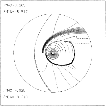
Figure 5: Discontinuity pattern: shock-capturing approach [75]

Although all the mentioned methods give essentially similar pattern of discontinuities in the computational region, we present here, for the convenience of the further discussion, the picture from [75]. The interstellar plasma number density of protons is assumed to be $\it n_{H+}\approx\rm 1\,cm^{-3}$. The velocity of LISM relative to the solar system is about $\it\rm 20\,km/s$, while the speed of sound of the LISM gas is about $\it\rm 10\,km/s$. Thus, LISM flow is supersonic. The SW charged particle number density is chosen $\it n_{H+}\approx\rm 10\,cm^{-3}$, its velocity is $\it V_{e}\approx\rm 500\,km/s$, the speed of sound $\it c_{e}\approx\rm 100\,km/s$ at the distance of the Earth’s orbit ($\it 1\,{\rm AU}$). The nondimensional parameters of the problem are Mach numbers of LISM and SW $\it M_{\infty}$, $\it M_{e}$, the relations of dynamic pressures $\it K=\rho_{e}V^{2}_{e}/\rho_{\infty}V^{2}_{\infty}$ and stagnation temperatures $\it\chi=T_{0e}/T_{0\infty}$ of SW and LISM. This corresponds to the following values of dimensionless parameters of the problem: $\it M_{\infty}=2$, $\it M_{e}=5$, $\it\chi=400$, $\it K=6250$. The specific heat ratios for SW and LISM are supposed to be 5/3. The calculation is performed in the ring region with the inner and outer circle radii being $\it R_{\rm min}=10$ and $\it R_{\rm max}=500\,{\rm AU}$ with 99 and 116 cells in the radial and in the angular direction, respectively. Constant pressure (below the symmetry axis) and constant density natural logarithm contours of the steady-state solution are presented in Fig. 5. Results are given in the polar region with the inner and outer circle radii 10 and $\it 400\,{\rm AU}$. All peculiarities are seen of the shock wave pattern shown schematically in Fig. 2.

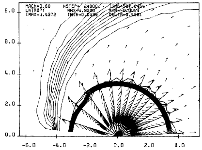
Figure 6: Entropy contours with velocity vectors for the model with the Mach number 0.6 [93]

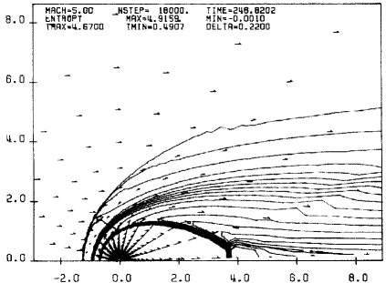
Figure 7: Entropy contours and velocity vectors for the Mach number 5 [93]

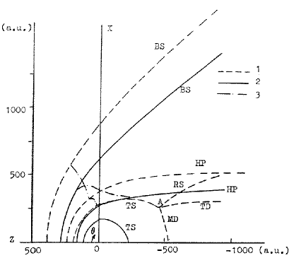
Figure 8: Geometrical pattern of the interface. Results of the numerical calculations for $\it n_{H\infty}=0(1)$ and $\it n_{H\infty}=\rm 0.14cm^{-3}(2)$; curves (3) are the sonic lines. Positions of the bow shock (BS), termination shock (TS), heliopause (HP), reflected shock (RS), tangential discontinuity (TD), and Mach disk (MD) are shown.

Calculations for a large variety of the stellar wind and interstellar medium parameters, including those very different from the parameters of the solar wind, were performed in [55] and [92]. These parametric studies may reflect various situations corresponding to ejecting stars and their environment. Although from the purely gasdynamic viewpoint the LISM flow is supersonic, the presence of the interstellar magnetic field and charge-exchange processes can decrease the effective Mach number of the uniform interstellar medium flow, thus making it subsonic. For this reason several authors [93], [97] performed calculations of a subsonic interaction on the basis of the Euler equations. It is quite clear that, unlike the two-shock Baranov’s model, no bow shock can appear in the stationary solution. As will be shown later, the termination shock in this case does not have a bullet shape and the difference between its stand-off distances in the upwind and in the downwind direction is not so pronounced. This can also be seen in Fig. 6, corresponding to $\it M_{\infty}=0.6$. If the stellar wind Mach number is larger than that of the solar wind, the termination shock becomes elongated in the backward direction and the size of the Mach disk diminishes (see Fig 7, corresponding to $\it M_{\infty}=5$). The latter two figures are taken from [93].

Summarizing the subject of this section, we would like to admit that, although application of shock-fitting methods can provide a solution with a very high precision at low computational costs, they can be used only in the flow regions with a simple shock-wave pattern which is known beforehand (say, the upwind part of the SW–LISM interaction). Attempts to promote calculations for larger distances into the downwind region results in the substantial distortion of the results, like it was in [113], in which the possibility of the Mach-type reflection of the termination shock was not taken into account. A shock-fitting method in its rigorous sense was not realized, since the exact relations connecting parameters in the triple point were not used. The best way out in this case is to combine shock-fitting and shock-capturing methods, as it was done in [11].

4 Stationary solutions including neutral particles

Since we restrict ourselves in this review to the description of numerical methods used to solve the SW–LISM interaction problem, more or less complete description of physical processes governing the charge exchange between the plasma and the neutral component of the flow lies beyond the scope of this work. It can be found in the corresponding references mentioned in Introduction. However, it is quite clear that the LISM is a partially ionized gas and, therefore, a consistent model must be developed accounting for the mutual influence of charged and neutral particles. Although both helium and hydrogen atoms are present, the authors usually disregard helium atoms, since their cosmic abundance is much less than that of hydrogen atoms.

The first attempts to estimate the influence of this process, say, [7] and [87], did not include the influence of the hydrogen atoms on the plasma component. The first self-consistent model of the heliospheric interface was suggested in [8]. In that paper the authors introduced the source terms accounting for the momentum and the energy transfer between the two components into the system of the Euler gasdynamic equations in the quasi-linear form. These source terms were presented in the form:

$$\rho\nu_{c}({\bf v}_{H}-{\bf v})$$ (34)

for the momentum equations (1) and

$$\rho(\gamma-1)\nu_{c}\left[{({\bf v}_{H}-{\bf v})^{2}\over 2}-{3kT\over 2m_{H}}+{3kT_{H}\over 2m_{H}}\right]$$ (35)

for the energy equation. Here $\it k$ is the Boltzmann constant and $\it m_{H}$ is the mass of the hydrogen atom. For the collision frequency between protons and atoms the following formula was used:

$$\it\it\nu_{c}={\rho_{H}\sigma Q\over m_{H}},\,Q=\left[({\bf v}_{H}-{\bf v})^{2}+{128k(T+T_{H})\over 9\pi m_{H}}\right]^{1\over 2},$$

where $\it\sigma$ is the effective charge-exchange cross-section.

The hydrogen atoms were assumed to conserve their velocity and temperature in the process of their interaction with protons and the origin of the secondary hydrogen atoms was neglected. That allowed to describe the behavior of neutrals in the region between the two shocks by the system

$$\it\displaystyle{\bf v}_{H}={\bf v}_{H_{\infty}}={\rm const},$$

$$\it\displaystyle T_{H}=T_{H_{\infty}}={\rm const},$$

$$\it\displaystyle\mathop{\rm div}\nolimits(\rho_{H}{\bf v}_{H})=-\rho\nu_{c}$$

Incorporating this source term into implicit method [4] does not represent any difficulty and the solution was obtained for various values of dimensionless parameters. The major effect of charge exchange on the heliospheric interfaces is to decrease the distances to the TS, HP, and BS. The original developers of the approach [8], which considers the flow of neutral particles as a hydrodynamic flow, themselves admitted in [9] its main drawbacks: (1) such description is hardly justifiable, since the mean free-path of the hydrogen atoms is not smaller than the characteristic length of the problem; (2) the Maxwellian distribution of the atoms was adopted to calculate the plasma momentum and energy losses. This was the reason of applying the Monte-Carlo method for simulation of the hydrogen atom trajectories [54]. It gives a possibility to evaluate the source terms in the momentum and the energy equations for the plasma component on the basis of the kinetic description of the hydrogen atoms. An iteration method [10] was proposed to solve both systems of equations. The numerical results are discussed in [11] and [12]. This approach is nowadays the only one which can be considered physically consistent from the viewpoint of computational fluid dynamics. In Fig. 8, the geometrical interface between the two flows is presented [11] reflecting the influence of the charge exchange processes. The picture is presented in the $\it X0Z$ plane, where $\it 0Z$ coincides with the axis of symmetry and is antiparallel to the vector on the LISM velocity (the Sun is in the coordinate system origin). The solid and the dotted lines in Fig. 8 correspond to $\it n_{H_{\infty}}$= $\it\rm 0.14\,cm^{-3}$ and $\it n_{H_{\infty}}=0$, respectively. The parameters of the plasma component were the following: $\it n_{e}=\rm 7\,cm^{-3}$, $\it V_{e}=\rm 450\,km/s$, $\it M_{e}=10$, $\it n_{\infty}=\rm 0.07\,cm^{-3}$, $\it V_{\infty}=\rm 25\,km/s$, and $\it M_{\infty}=2$. One can see a large influence of the described processes on the flow pattern and it is quite clear that any realistic calculation of the problem must take them into consideration.

Recently in [70] and [115] the simplified approach [8] was modified by developing the multifluid description for the neutrals which tried to take into account the highly non-Maxwellian nature of the neutral distribution. Since in these papers the plasma was assumed Maxwellian only in each region between the discontinuity surfaces, the neutral population produced by the charge exchange in these regions has the same basic characteristics as those of the plasma component. Although this approach still remains approximate, one must admit that it allowed its developers to obtain the solutions of the three-dimensional and nonstationary problems which have not been solved yet on the basis of the Monte-Carlo method.

5 Hydrodynamic instabilities in the SW–LISM interaction

As was admitted in [106], the contact discontinuity between the inner and the outer subsonic region is potentially the subject to the fluid Kelvin–Helmholtz or MHD flute instabilities which could produce some of the inhomogeneous structures of astropause tails. The study of instabilities accompanying the problem of the SW–LISM interaction with and without magnetic field is an important independent task which lies outside the scope of this review. We are going to clarify here only the effect of the choice of numerical methods on their origin and development in the problem in which two flows possessing substantially different entropies collide at a contact surface calculated by shock-capturing methods. It is more or less clear that discontinuity-fitting methods are hardly applicable for this task.

As was convincingly shown in [58] and [93], complicated nonstationary patterns can be obtained owing to the Rayleigh–Taylor instabilities if the interaction is accompanied by the gravitational effect from the star. In the case of the solar wind the gravity can be neglected, since the Hoyle–Littleton accretion radius is about 4.5 AU, which is much smaller than the expected location of the termination shock. In [55], however, the stellar wind–interstellar medium interaction was studied for parameters different from those corresponding to the solar wind and the results were obtained clearly indicating instability of the flow. The Osher numerical scheme [24] was used and an algebraically generated irregular grid rather than the polar one applied in the previous study of the problem [93]. That type of the grid is supposed to give a finer resolution at large distances from the ejecting center. The influence of the interstellar medium Mach number was studied in a wide range from $\it M_{\infty}=0.6$ to 15. A highly nonstationary solution was obtained in this case, instabilities originating both near the astropause stagnation point and in its lateral region (Fig. 9).

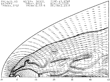
Figure 9: Entropy contours and velocity vectors [55] ($\it M_{\infty}=15$)

The Kelvin–Helmholtz instability in the latter region are quite possible as the gases with different entropy move along the both sides of a contact surface at different speeds. The origin of the Kelvin–Helmholtz instability near the stagnation point, however, is questionable, since velocities are very small there. Such stagnation point instabilities, however, were found earlier in the calculations of astrophysical jets [65], [66], and [95]. Similar instabilities were also found in [56] and [57] in the calculations of opposing and forward-facing jets. They were also observed in the experiments [36], [90], and [91]. It is worth mentioning, however, that the instabilities of the latter type were not obtained in the calculations for parameters close to the solar wind – interstellar medium interaction, as was reported in [96]. Moreover, N. Pogorelov in his calculations occasionally obtained instabilities near the stagnation point, even for a rather rough mesh, using the Roe-type MUSCL scheme under unfavorable selection of the parameter reconstruction method. Note that one or another parameter interpolation based on the assumption of the linear, parabolic [25], or higher-order distributions inside computational cells is usually used to increase the order of accuracy of the chosen numerical scheme. Say, in [75] and [76] the interpolation of characteristic variables was used which had been discovered to give much more stable results in the vicinity of the geometrical singularities at $\it\theta=0$ and $\it\theta=\pi$. Note that both the polar grid used in [76] and the algebraically generated O-type grid incorporated into the algorithm [55] possess such a singularity. In [80] the choice of the form of governing equations (2) or (3) was claimed to have a certain effect on the stability of results.

There also exits another aspect of the problem. As was mentioned in the previous section, the interaction between the interstellar atoms and the solar plasma ions via resonant charge-exchange collisions greatly affects the steady-state structure of the global heliosphere. The flow of interstellar ions is diverted around the nose of the heliopause, whereas the neutral particles penetrate into the heliosphere impeded aside from the charge-exchange collisions. Thus, there is a velocity difference between them near the nose which performs like a drag force acting on the plasma (see Eq. 28). Since the LISM density is larger at the heliopause than that of the SW, the contact surface is potentially Rayleigh–Taylor unstable. That kind of instability was admitted in [52] and [115]. Its origin was confirmed by several numerical experiments, including the one applying the entirely different particle-in-cell code [20], and by comparing the instability linear growth rate with the theoretical one. However, as was admitted earlier, the multifluid hydrodynamic model in which all fliuds were supposed to be in a local thermal equilibrium was used in the above-mentioned papers to determine the motion of the neutral particles. This makes the obtained results questionable from the viewpoint of the spatial scale of instabilities. Paper [52] also neglects the effect of energetic solar wind neutrals created by the charge exchange inside the heliopause. The drag force caused by these neutrals tends to compensate the inward force described earlier and partially suppress the instability.

The study of hydrodynamic instabilities originating in the SW–LISM interaction problem is far from its conclusion also due to a number of physical phenomena that can affect it, such as, the interstellar magnetic field, cosmic rays, etc. It is important to admit in this review that, investigating instabilities, one must be very careful in order to distinguish those of physical and of numerical origin.

6 Nonstationary SW–LISM interaction

As was mentioned above and is widely accepted, the solar wind changes its speed from supersonic to subsonic through a termination shock. A number of reasons can cause temporal asymmetries of the termination shock and, therefore, the interaction pattern as a whole. Among them are disturbances of the solar wind and its 11-year periodicity. Due to these reasons the heliospheric shock will move in response to variation in upstream solar wind conditions. In [100], a kinematic analysis is made of the solar wind driven temporal variations in the heliospheric termination shock distance. In [15], [16], and [63] the motion of this shock was analyzed analytically on the basis of one-dimensional gasdynamic model. It was admitted that the termination shock would rather be nonstationary and would resemble a distorted asymmetric balloon with some part moving inward and others moving backward. In [97] the termination shock response to large-scale solar wind fluctuations were studied numerically using the Lax–Wendroff scheme. The LISM flow was assumed subsonic. In [47], on the basis of the similar numerical method 11-year solar wind variation influence on the inner shock was investigated. In [75] and [76] nonstationary problems were modeled by a numerical solution of the Euler gasdynamic equations (2) in the finite-volume formulation (21) using a MUSCL-type TVD high-resolution numerical scheme. The suggestion was made of a piecewise-linear distribution of the characteristic parameters inside the cells to determine the values at their boundaries and slope limiters were used to attain a TVD property. The results presented below were obtained using the formulas [1]:

$$\it\displaystyle\bar{\bf E}_{l+1/2,n}=\bar{\bf E}({\bf U}^{L},{\bf U}^{R}),$$ (36)

$$\it\displaystyle{\bf U}^{L}={\bf U}_{l,n}+{\bf U}^{\prime}_{l,n}\mathchar 1\relax R/2,$$

$$\it\displaystyle{\bf U}^{R}={\bf U}_{l+1,n}-{\bf U}^{\prime}_{l+1,n}\mathchar 1\relax R/2,$$

$$\it\displaystyle{\bf U}^{\prime}_{l,n}=S_{l,n}{\bf W}^{\prime}_{l,n},$$

$$\it\displaystyle{\bf W}^{\prime}_{l,n}={(b^{2}_{m}+c)a_{m}+(a^{2}_{m}+c)b_{m}\over a^{2}_{m}+b^{2}_{m}+2c},$$

$$\it\displaystyle{\bf a}=S^{-1}_{l,n}({\bf U}_{l+1,n}-{\bf U}_{l,n}),$$

$$\it\displaystyle{\bf b}=S^{-1}_{l,n}({\bf U}_{l,n}-{\bf U}_{l-1,n})$$

Here $\it c$ is a small positive value used to avoid division by zero. In these formulas $\it S$ and $\it S^{-1}$ are $\it(4\times 4)$ matrices, constructed using right and left eigenvectors of the Jacobian matrix $\it\partial\bar{\bf E}/\partial{\bf U}$.

The fluxes presented by Eq. (30) were defined on the basis of Roe’s approximate Riemann solver [88].

Fluxes through another pair of cell surfaces can be obtained similarly.

The promotion of the solution in time was performed in the following way:

$$\it\displaystyle{\bf U}^{(1)}_{l,n}={\bf U}^{k}_{l,n}+{\mathchar 1\relax t\over 2}\,{\partial{\bf U}^{k}_{l,n}\over\partial t};$$

$$\it\displaystyle{\bf U}^{k+1}_{l,n}={\bf U}^{k}_{l,n}+\mathchar 1\relax t\,{\partial{\bf U}^{(1)}_{l,n}\over\partial t},$$

where $\it t=k\,\mathchar 1\relax t$, $\it k=0,1,\ldots\,$, and $\it\mathchar 1\relax t$ is defined by the time resolution and by the CFL condition.

The LISM proton number density was assumed to be $\it n_{H+}=\rm 1\,cm^{-3}$. The velocity of LISM relative to the solar system is about $\it\rm 20\,km/s$, while the speed of sound of the LISM gas is about $\it\rm 10\,km/s$. The SW protons number density was adopted $\it n_{H+}=\rm 10\,cm^{-3}$, while its velocity is $\it V_{e}\approx\rm 500\,km/s$, the speed of sound $\it c_{e}\approx\rm 100\,km/s$ at the distance of the Earth’s orbit ($\it 1\,{\rm AU}$). This corresponds to the following values of dimensionless parameters chosen for the initial data: $\it M_{\infty}=2$, $\it M_{e}=5$, $\it\chi=400$, $\it K=6250$. The stationary initial flow was obtained by the same numerical method using a time-stabilization approach. The calculation was performed in the ring region with the inner and outer circle radii being $\it R_{\rm min}=10$ and $\it R_{\rm max}=500\,{\rm AU}$. On the inner surface all parameters were specified as functions of time by formulas:

$$\it\displaystyle U=25,\quad\rho(t)=\rho(0)(1+4\exp[-(t-3)^{2}]),$$

$$\it\displaystyle p(t)=3.2325\rho^{\gamma}(t),$$

since this boundary is supersonic. Here $\it U$ is the radial velocity component. Although the choice of parameters is somewhat nonrealistic, as far as the solar wind is concerned, it still can be used for a qualitative analysis of a nonstationary picture of the interaction.

The initial distributions of pressure (below the symmetry axis) and density logarithms are shown in Fig. 5. The size of the outer circle in the figures is 400 AU. Similar isolines are presented in Figs. 10–13 at different moments of time (in the units $\it 1\,{\rm AU}/U_{\infty}$). The growing part of the disturbance, interacting with the inner shock, moves it, first, from the centre, Fig. 10, the intensity of IS increasing. Later, it tends to achieve the initial position.

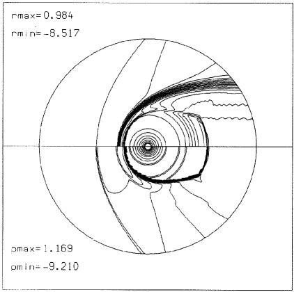
Figure 10: Pressure and density logarithm isolines [75], $\it t=8$

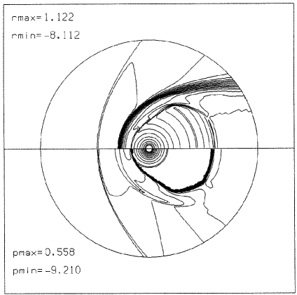
Figure 11: Pressure and density logarithm isolines [75], $\it t=12$

The penetration of the disturbance in the region between IS and CD is seen on both charts of isolines at different moments of time. The disturbance, while crossing IS, increases greatly, and after some time a local pressure maximum originates between IS and CD (Fig. 11). This leads to the effect of suction of SW gas to the centre accompanying IS motion in the same direction. This pressure extremum line gradually moves towards CD, see Figs. 12–13.

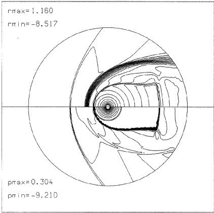
Figure 12: Pressure and density logarithm isolines [75], $\it t=18$

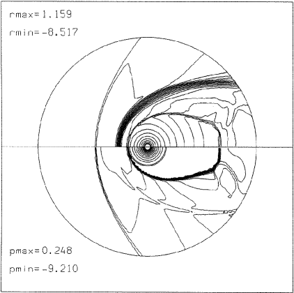
Figure 13: Pressure and density logarithm isolines [75], $\it t=21$

The parts of the computational region more remote from the source position suffer the same changes later in time.

As soon as the disturbance meets different points of IS, the latter suffers substantial distortion. When the triple point on IS is reached, there appear two triple points with different reflected shocks and recirculation zone between them (Fig. 13). As soon as the source intensity becomes constant, the position of IS gradually, but rather slowly, moves towards its initial position. The maximum increase of MD stand-off distance is greater than that of IS along the ray $\it\theta=0$.

The relaxation of the flow towards some stationary solution is very slow ($\it t>220$). When $\it t>20$, in the region near $\it\theta=0$ additional local pressure extrema vanish. The extended vortex region originates behind MD and it is up to $\it t=60$, when these vortices vanish, probably due to numerical viscosity.

Now we present some results [76] concerning the periodic SW–LISM interaction. In this calculation the LISM proton number density, its velocity and the speed of sound are $\it n_{\infty}=\rm 0.1\,cm^{-3}$, $\it V_{\infty}=\rm 20\,km/s$ and $\it c_{\infty}=\rm 10\,km/s$, respectively. Parameters of the solar wind change substantially within the 11-year period of the solar activity. The concentration of charged particles $\it n_{e}=\rm 1.56\,cm^{-3}$ and the radial SW velocity $\it V_{e}=\rm 400\,km/s$ are chosen for the minimum of the solar activity, while $\it n_{e}=\rm 8\,cm^{-3}$ and $\it V_{e}=\rm 500\,km/s$ correspond to its maximum (see [6] and [21]). Thus, for dimensionless parameters we have $\it K=6250$, $\it\chi=256$, $\it M_{\infty}=2$, and $\it M_{e}=5$ in the minimum and $\it K=50000$, $\it\chi=400$, $\it M_{\infty}=2$, and $\it M_{e}=5$ in the maximum of the solar activity. These values are chosen as the basic points for the sine function approximating the time dependence of $\it K$ and $\it\chi$ within 11 years. The dimensionless time unit is 86.8 days. The time step is chosen to be $\it\mathchar 1\relax t\approx 0.4$ days. Parameter distribution corresponding to the stationary solution in the minimum solar activity is chosen as initial data. The results are obtained by the MUSCL numerical method described above. The calculation is performed in the ring region with the inner and the outer circle radii being $\it R_{\rm min}=14$ and $\it R_{\rm max}=700$, respectively.

The isolines of the pressure (below the symmetry axis) and the density logarithms corresponding to the initial data are shown in Fig. 14. They are presented for the outer circle size equal to 560 AU. The number of cells is 99 and 116 in the radial and in the angular direction, respectively. At the initial stage of the flow development, the increase of the parameter $\it K$ results in the TS motion from the Sun. The motion of the compression wave through TS causes the origin of a new shock wave propagating from the center. This can be seen in Fig. 15 corresponding to $\it t=20$. This shock penetrates through the contact discontinuity and moves towards the bow shock, see Fig. 16 ($\it t=36$).

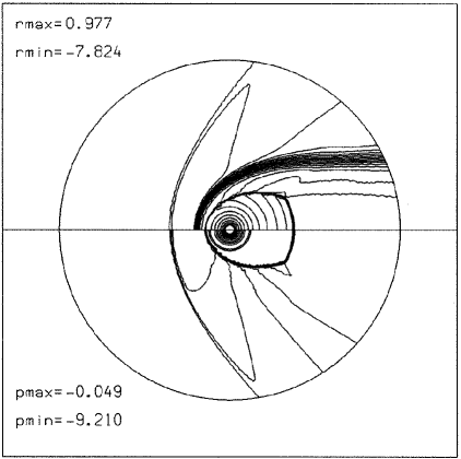
Figure 14: Pressure and density logarithm isolines [76], $\it t=0$

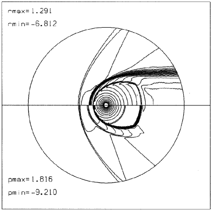
Figure 15: Pressure and density logarithm isolines [76], $\it t=20$

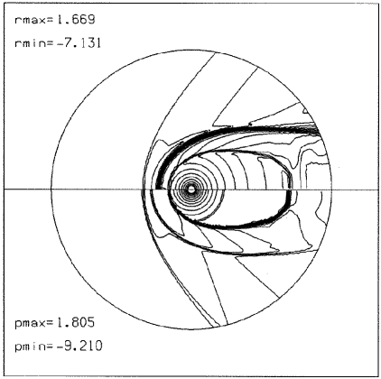
Figure 16: Pressure and density logarithm isolines [76], $\it t=36$

The decreasing part of the periodic function causes a backward motion of the termination shock towards the Sun. This leads to the origin of new flow division surfaces, reverse flow zones, and vortices of variable size and intensity in the wake region. At $\it t=60$, see Fig. 17, the size of the bullet shape termination shock becomes minimum again. Later on a next nonstationary shock wave appears, etc. A definite 11-year periodicity is developed in the shape of the termination shock. Parameter distribution between the inner and the bow shock is determined by the propagation of shock waves traveling one after another and interacting with the less intensive waves reflected from the bow shock (Fig. 18).

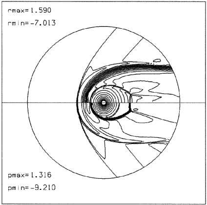
Figure 17: Pressure and density logarithm isolines [76], $\it t=60$

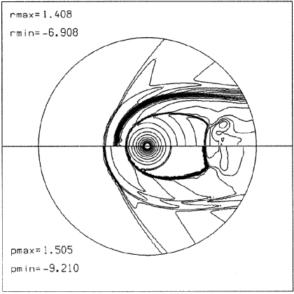
Figure 18: Pressure and density logarithm isolines [76], $\it t=84$

This modeling shows that the flow pattern is substantially nonstationary which must be taken into account when analyzing responses from the space vehicles crossing these discontinuities. Variable solar activity is usually accompanied by the asymmetry of the solar wind which will be considered in the next section.

Application of a high-resolution numerical methods allows one to avoid spurious oscillations near shocks and provides their sharper resolution using smaller number of computational cells than it is necessary in nonmonotone schemes with artificial viscosity.

7 Nonuniform solar wind – interstellar medium interaction

Distant solar wind deviations from spherical symmetry induced by the interaction with neutral interstellar hydrogen due to photoionization and charge-exchange processes were studied in [40] by a perturbation technique. The penetration of neutral particles deep inside the heliosphere results in a substantial increase of the distant solar wind temperature. In all models described in the previous sections we considered the stellar (solar) wind as spherically-symmetric. It can fairly easily become asymmetric, since charge-exchange processes are clearly more effective in the forward region of the interaction because their efficiency is proportional to the velocity difference between neutral and charged particles. The perturbation analysis has shown that a strongly asymmetric distribution of the neutral hydrogen within the heliosphere causes asymmetric deceleration and extremely nonuniform distribution of the distant solar wind temperature, thus leading to non-radial gradients and flows.

This is, however, only one (external) reason of the solar wind asymmetry. Another one is determined by a mere variation of the solar wind symmetry in time within its 11-year activity period (see, e.g., speculations in [76]). According to the solar minimum observations by Ulysses, the solar wind parameters depend on the helioaltitude. These data (see [72] and [73]) indicate that two large polar coronal holes, one in the northern and the other in the southern hemisphere, produce a hotter, lower-density, higher-speed wind comparing with the ecliptic wind. In [71] the calculations were performed of a nonuniform solar wind–interstellar medium interaction using the earlier mentioned three-dimensional time-dependent ZEUS method [98]. The solar wind boundary conditions were taken from the published Ulysses data. According to them, the ram pressure increases 1.5 times from the ecliptic plane to the solar pole. That is why, the termination shock in the calculations was found to be elongated along the solar axis which, in turn, resulted in an increased flow in the ecliptic plane compared with that over the solar poles. The authors reported a pronounced effect of the solar wind asymmetry on the global structure of the termination shock and heliopause. Both a two-shock (supersonic LISM) and a one-shock (subsonic LISM) model were considered. It is worth mentioning once again in this connection that, if only the motion of charged particles is considered, the LISM flow is definitely supersonic. Pure gasdynamic subsonic models for the problem under consideration are sometimes used to account for the net effect of the charge-exchange processes, the influence of cosmic rays [35], and interstellar magnetic field. The latter subject will be discussed in the next section.

The paper [71] definitely indicates, from our viewpoint, that any realistic model for the SW–LISM interaction must include both neutral particles, the asymmetry of the solar wind, and, as a consequence, the solar wind periodicity, since the asymmetry varies within the solar activity period. This, of course, does not prevent an investigation of different physical effects separately.

8 Solar wind interaction with the magnetized interstellar medium

The presence of the interstellar magnetic field necessitates solution of the MHD equations for modeling of the SW–LISM interaction. The influence of magnetic field becomes important if a magnetic pressure $\it{\bf B}^{2}/8\pi$ becomes comparable with a dynamic pressure. Magnetic field causes an increase of the maximum speed of small perturbations in the LISM flow, especially in the direction normal to the direction of the magnetic field, thus resulting in the decrease of the effective Mach number [33] and [34]. Though the magnitude and the direction of the interstellar magnetic field is not perfectly known, the estimates from [3] indicate the possible importance of its presence. The value and the direction of the LISM magnetic field can affect the global structure of the interaction not only directly, but also by modulating the distance between the bow shock and the heliopause which determines the transparency of this layer for the LISM neutrals. This, in turn, affects the observed line profiles of the solar Lyman-$\it\alpha$ backscattered emission and estimates of the LISM parameters (see the discussion in [12] and [50]). If the LISM magnetic field is not parallel to its velocity, the problem becomes three-dimensional. Later in the section we discuss the results of such MHD modeling.

It is worth mentioning, that although the value of the solar magnetic field is often neglected in numerical modeling of the problem under consideration at the distances of the termination shock, its influence is substantial at Earth’s magnetosphere distances [68] and [109]. In [107] the global structure of the outer heliosphere was studied in the axisymmetric formulation for a subsonic interstellar medium with taking into account a time-varying poloidal magnetic field. In [108] and [67] the toroidal magnetic field in the heliosheath was found to increase with the distance from the Sun. The complicated three-dimensional nostationary behavior of the flow was studied which showed the importance of taking this component of the magnetic field into account. We restrict ourselves to noting this aspect of the problem and will not discuss it below.

8.1 On the eigenvector and eigenvalue systems of MHD equations

The system of ideal MHD equations in the conservation-law form is presented by Eq. (1). This system can be directly rewritten in the quasi-linear form which is more convenient for the characteristic analysis. It is well-known that the equation $\it\mathop{\rm div}\nolimits{\bf B}=0$ expresses the absence of magnetic charge. It is also evident that, if magnetic charge is absent initially, it will not appear mathematically at any time instant. From this viewpoint the above equation is excessive. If we rewrite the system of MHD equations [51]

$$\it\displaystyle{\partial\rho\over\partial t}+\mathop{\rm div}\nolimits\rho{\bf v}=0,$$

$$\it\displaystyle{\partial{\bf v}\over\partial t}+({\bf v}\cdot\nabla){\bf v}=-{\nabla p\over\rho}-{{\bf B}\times\mathop{\rm rot}\nolimits{\bf B}\over 4\pi\rho},$$

$$\it\displaystyle{dp\over dt}=a{d\rho\over dt}$$

$$\it\displaystyle\frac{\partial{\bf B}}{\partial t}=\mathop{\rm rot}\nolimits({\bf v}\times{\bf B})$$

in quasilinear form not paying attention to the condition $\it\mathop{\rm div}\nolimits{\bf B}=0$, the following system is obtained ($\it a$ is the acoustic speed of sound):

$${\partial{\bf u}\over\partial t}+A_{1}\,{\partial{\bf u}\over\partial x}+A_{2}\,{\partial{\bf u}\over\partial y}+A_{3}\,{\partial{\bf u}\over\partial z}=\mathchar 1584\relax\,,$$ (37)

where

$$\it\it{\bf u}=\left(\rho,\,u,\,v,\,w,\,p,\,B_{x},\,B_{y},\,B_{z}\right)^{T},$$

$$\it\it A_{1}=\left(\begin{array}[]{cccccccc}u&\rho&0&0&0&0&0&0\\ 0&u&0&0&{1\over\rho}&0&{B_{y}\over 4\pi\rho}&{B_{z}\over 4\pi\rho}\\ 0&0&u&0&0&0&-{B_{x}\over 4\pi\rho}&0\\ 0&0&0&u&0&0&0&-\frac{B_{x}}{4\pi\rho}\\ 0&\rho a^{2}&0&0&u&0&0&0\\ 0&0&0&0&0&u&0&0\\ 0&B_{y}&-B_{x}&0&0&0&u&0\\ 0&B_{z}&0&-B_{x}&0&0&0&u\end{array}\right)\!,$$

$$\it\it A_{2}=\left(\begin{array}[]{cccccccc}v&0&\rho&0&0&0&0&0\\ 0&v&0&0&0&-{B_{y}\over 4\pi\rho}&0&0\\ 0&0&v&0&\frac{1}{\rho}&{B_{x}\over 4\pi\rho}&0&{B_{z}\over 4\pi\rho}\\ 0&0&0&v&0&0&0&-\frac{B_{y}}{4\pi\rho}\\ 0&0&\rho a^{2}&0&v&0&0&0\\ 0&-B_{y}&B_{x}&0&0&v&0&0\\ 0&0&0&0&0&0&v&0\\ 0&0&B_{z}&-B_{y}&0&0&0&v\end{array}\right)\!,$$

$$\it\it A_{3}=\left(\begin{array}[]{cccccccc}w&0&0&\rho&0&0&0&0\\ 0&w&0&0&0&-{B_{z}\over 4\pi\rho}&0&0\\ 0&0&w&0&0&0&-{B_{z}\over 4\pi\rho}&0\\ 0&0&0&w&\frac{1}{\rho}&\frac{B_{x}}{4\pi\rho}&\frac{B_{y}}{4\pi\rho}&0\\ 0&0&0&\rho a^{2}&w&0&0&0\\ 0&-B_{z}&0&B_{x}&0&w&0&0\\ 0&0&-B_{z}&B_{y}&0&0&w&0\\ 0&0&0&0&0&0&0&w\end{array}\right)\!,$$

Solution of the characteristic equation

$$\it\it\mathop{\rm det}\nolimits(A_{1}-\lambda I)=0$$

gives the following eigenvalues:

$$\it\displaystyle\lambda_{1,2}=u,\quad\lambda_{3,4}=u\pm\frac{B_{x}}{\sqrt{4\pi\rho}},$$ (38)

$$\it\displaystyle\lambda_{5,6,7,8}=u\pm{1\over 2}\biggl{[}\biggl{(}a^{2}+\frac{{\bf B}^{2}}{4\pi\rho}+\frac{B_{x}a}{\sqrt{\pi\rho}}\biggr{)}^{1/2}$$

$$\it\displaystyle\pm\biggl{(}a^{2}+\frac{{\bf B}^{2}}{4\pi\rho}-\frac{B_{x}a}{\sqrt{\pi\rho}}\biggr{)}^{1/2}\biggr{]}$$ (39)

Note that in one-dimensional treatment the equation for $\it B_{x}$ reduces to

$${\partial B_{x}\over\partial t}+u{\partial B_{x}\over\partial x}=0,$$ (40)

that is, to the one-dimensional convection equation for $\it B_{x}$. Of course, in the truly one-dimensional problem (all values depend only on the spatial variable $\it x$) one can simply assume $\it B_{x}\equiv\mathop{\rm const}\nolimits$ and omit the corresponding equation. On the contrary, if we are going to apply the solution of the one-dimensional MHD Riemann problem to determine the flux through the cell boundary, such an assumption is too excessive, since only the integral $\it\oint B_{n}d\sigma$ over the whole computational cell must be equal to zero. Among eigenvalues (32)–(33) the first two correspond to the entropy and $\it B_{x}$ convection waves, $\it\lambda_{3,4}$ corresponds to the Alfvén, or rotational, waves, and the other ones to the slow and to the fast magnetosonic wave. Omitting Eq. (34), we reduce the system to $\it 7\times 7$. Both the extended $\it 8\times 8$ system and the reduced one have real eigenvalues and a degenerate set of eigenvectors. One can easily derive expressions for them. Otherwise, one can refer to [22], [83], and [101]. As was admitted in [39] and [84], we can use the extended system to derive an approximate solution to the MHD Riemann problem. Another possibility is to derive formulas for the $\it 7\times 7$ system and use a convection equation to find $\it B_{x}$ ($\it x$ is normal to the cell boundary) on the cell surface. It is also useful to realize that by collecting the source term from system (31) to arrive at the conservative form similar to (1), we obtain the following system:

$${\partial{\bf U}\over\partial t}+{\partial{\bf E}\over\partial x}+{\partial{\bf F}\over\partial y}+{\partial{\bf G}\over\partial z}+{\bf H_{\rm div}}=\mathchar 1584\relax\,,$$ (41)

where

$$\it\it{\bf H_{\rm div}}=\mathop{\rm div}\nolimits{\bf B}\left(0,\,{B_{x}\over 4\pi},\,{B_{y}\over 4\pi},\,{B_{z}\over 4\pi},\,{{\bf v}\cdot{\bf B}\over 4\pi},\,u,\,v,\,w\right)^{\rm T}$$

This form of the system will be used later to satisfy the divergence-free condition.

Since the application of high-resolution numerical schemes to MHD flows and to the problem under consideration, in particular, has not yet become common (see some tests in [103]), we give their description in the next subsection.

8.2 High-resolution numerical schemes for MHD equation

TVD upwind and symmetric differencing schemes have recently become very efficient tool for solving complex multi-shocked gasdynamic flows. This is due to their robustness for strong shock wave calculations. A general discussion of the modern high-resolution shock-capturing methods and their application for a variety of gasdynamic problems can be found in [42] and [112]. The extension of these schemes to the equations of the ideal magnetohydrodynamics (MHD) is not straightforward. First, the exact solution [49] of the MHD Riemann problem is too multivariant to be used in regular calculations. Second, several different approximate solvers [22], [23], [26], [41], [77], [84], and [114] applied to MHD equations are now at the stage of investigation and comparison.

The schemes [22], [23], [41], and [77], [84] are based on the MHD extensions of Roe’s linearization procedure [88]. In [22], the attempt of such extension was made and the second order upwind scheme was constructed that demonstrated several advantages in comparison with the Lax–Friedrichs, the Lax–Wendroff, and the flux-corrected transport scheme [30]. Roe’s procedure, however, turned out to be realizable only for the special case with the specific heat ratio $\it\gamma=2$. The reason of such behavior of MHD equations is that there is not any single averaging procedure to find a frozen Jacobian matrix of the system. Another linearization approach is used in [23], [41], [77], and [84] in which the linearized Jacobian matrix is not a function of a single averaged set of variables, but depends in a complicated way on the variables on the right- and on the left-hand side of the computational cell surface. In [79] and [82] this procedure was shown to be nonunique. A multiparametric family of linearized MHD approximate Riemann problem solutions was presented that assured an exact satisfaction of the conservation relations on discontinuities. A proper choice of parameters is necessary to avoid physically inconsistent solutions.

Consider the one-dimensional system of MHD equations

$${\partial{\bf U}\over\partial t}+{\partial{\bf F}\over\partial x}=\mathchar 1584\relax,$$ (42)

where $\it{\bf U}=\left(\rho,\,\rho u,\,\rho v,\,\rho w,\,e,\,B_{y},\,B_{z}\right)^{\rm T}$ and

$$\it\it{\bf F}({\bf U})=\left(\begin{array}[]{c}\rho u\\ \rho u^{2}+p_{0}-B_{x}^{2}/4\pi\\ \rho uv-B_{x}B_{y}/4\pi\\ \rho uw-B_{x}B_{z}/4\pi\\ (e+p_{0})u-(uB_{x}+vB_{y}+wB_{z})B_{x}/4\pi\\ uB_{y}-vB_{x}\\ uB_{z}-wB_{x}\end{array}\right)$$

In these formulas $\it e=p/(\gamma-1)+\rho(u^{2}+v^{2}+w^{2})/2+(B_{x}^{2}+B_{y}^{2}+B_{z}^{2})/8\pi$ is the total energy per unit volume, $\it p_{0}=p+(B_{x}^{2}+B_{y}^{2}+B_{z}^{2})/8\pi$ is the total pressure, $\it p$ and $\it\rho$ are pressure and density, $\it{\bf v}=(u,v,w)$ is the velocity vector, $\it{\bf B}=(B_{x},B_{y},B_{z})$ is the magnetic field vector, and $\it\gamma$ is the adiabatic index. We assume all functions to depend only on time $\it t$ and on the linear coordinate $\it x$. Our aim is to construct a solution to Eq. (36) for $\it t>0$ for the piecewise-constant initial distribution of $\it\bf U$: $\it{\bf U}={\bf U}_{1}$ for $\it x<0$ and $\it{\bf U}={\bf U}_{2}$ for $\it x>0$. It is assumed, owing to the divergence-free condition, that $\it B_{x}=B_{x1}=B_{x2}\equiv{\rm const}$.

Let us first find the exact expression for the matrix $\it A=\mathchar 1\relax{\bf F}/\mathchar 1\relax{\bf U}$, where $\it\mathchar 1\relax{\bf U}={\bf U}_{1}-{\bf U}_{2}$ and $\it\mathchar 1\relax{\bf F}={\bf F}_{1}-{\bf F}_{2}$. The function $\it\bf F$ being nonlinear, the expression for $\it A$ is determined nonuniquely. In fact, if we choose some nondegenerate substitution $\it{\bf s}={\bf s}({\bf U})$, then from the exact equalities $\it\mathchar 1\relax{\bf F}=A_{F}\mathchar 1\relax{\bf s}$ and $\it\mathchar 1\relax{\bf U}=A_{U}\mathchar 1\relax{\bf s}$ it follows that $\it A=A_{F}(A_{U})^{-1}$. The exact analytic expressions for $\it A_{F}$ and $\it A_{U}$ can be written out explicitly if $\it\bf U$ and $\it\bf F$ are fractional linear functions of $\it\bf s$ or polynomials with respect to its components. We use here the equivalent transforms of the type $\it\mathchar 1\relax(BC)=\frac{1}{2}(B_{1}+B_{2})\mathchar 1\relax{}C+\frac{1}{2}(C_{1}+C_{2})\mathchar 1\relax{}B$. The structure and the simplicity of $\it A$ depends on the choice of $\it\bf s$. The matrix $\it A$ is an approximation to the Jacobian matrix $\it\displaystyle J=\frac{\partial{\bf F}}{\partial{\bf U}}$ and must conserve the main hyperbolic properties of $\it J$. It must be representable in the form $\it A=\mathchar 10\relax_{R}\mathchar 3\relax\mathchar 10\relax_{L}$, where $\it\mathchar 10\relax_{L}$ and $\it\mathchar 10\relax_{R}$ are the matrices of its left and right eigenvectors, respectively, $\it\mathchar 10\relax_{R}\mathchar 10\relax_{L}=I$, and $\it I$ is the identity matrix; $\it\mathchar 3\relax=||\lambda_{i}\delta_{ij}||$ is the diagonal matrix of the real eigenvalues of $\it A$, and $\it\delta_{ij}$ is the Kronecker delta.

Then the sought solution to Eq. (36) for $\it t>0$ acquires the form

$$\it\displaystyle{\bf U}(\xi) \it\displaystyle= \it\displaystyle\frac{1}{2}({\bf U}_{1}+{\bf U}_{2}+\mathchar 10\relax_{R}S(\xi)\mathchar 10\relax_{L}\mathchar 1\relax{\bf U}),$$ (43)

$$\it\displaystyle{\bf F}(\xi) \it\displaystyle= \it\displaystyle\frac{1}{2}({\bf F}_{1}+{\bf F}_{2}+\mathchar 10\relax_{R}|\mathchar 3\relax(\xi)|\mathchar 10\relax_{L}\mathchar 1\relax{\bf U})$$ (44)

where $\it\xi=\frac{x}{t}$, $\it S(\xi)=||\mathop{\rm sgn}\nolimits(\lambda_{i}-\xi)\delta_{ij}||$, and $\it|\mathchar 3\relax(\xi)|=||\lambda_{i}\mathop{\rm sgn}\nolimits(\lambda_{i}-\xi)\delta_{ij}||$. Equations (37) and (38) determine the piecewise-constant functions $\it{\bf U}(\xi)$ and $\it{\bf F}(\xi)$ that glue the right and the left values of the initial distributions via the system of jumps. If the Hugoniot-type condition is valid $\it\mathchar 1\relax{\bf F}=\lambda\mathchar 1\relax{\bf U}$, where $\it\lambda$ is the jump velocity, then $\it\lambda$ is one of the eigenvalues of $\it A$, since $\it\mathchar 1\relax{\bf F}-\lambda\mathchar 1\relax{\bf U}=(A_{F}-\lambda A_{U})\mathchar 1\relax{\bf s}=(A-\lambda E)A_{U}\mathchar 1\relax{\bf s}=(A-\lambda E)\mathchar 1\relax{\bf U}=0$. Thus, $\it\mathop{\rm det}\nolimits(A-\lambda E)=0$, $\it\mathchar 1\relax{\bf U}\neq 0$ is the eigenvector of $\it A$, and relations (37)–(38) describe the jump exactly.

The solution of this kind was first constructed for the equations of ideal gas dynamics [88]. In [22] such solution was given for Eq. (36) in the case $\it\gamma=2$. The approximate solution for an arbitrary adiabatic index was proposed in [41]. Here we present the procedure for obtaining the extension of Roe’s linearization procedure for MHD equation and show that it is not unique. Thus, the solution from [41] is the particular case of the multiparametric family of approximate solutions to the MHD Riemann problem.

We choose the vector $\it\bf s$ as a generalization of that for pure gas dynamics:

$$\it\it{\bf s}=\left(\begin{array}[]{c}R\\ U\\ V\\ W\\ {\cal I}\\ Y\\ Z\end{array}\right)=\left(\begin{array}[]{c}\sqrt{\rho}\\ \sqrt{\rho}u\\ \sqrt{\rho}v\\ \sqrt{\rho}w\\ \sqrt{\rho}H\\ B_{y}/\sqrt{\rho}\\ B_{z}/\sqrt{\rho}\end{array}\right)$$

Then

$$\it\it{\bf U}=\left(\begin{array}[]{c}R^{2}\\ RU\\ RV\\ RW\\ U_{5}\\ RY\\ RZ\end{array}\right),$$

where

$$\it\displaystyle U_{5} \it\displaystyle= \it\displaystyle\frac{R{\cal I}}{\gamma}+\frac{(U^{2}+V^{2}+W^{2})(\gamma-1)}{2\gamma}$$

$$\it\displaystyle- \it\displaystyle\frac{(Y^{2}+\nobreak Z^{2})R^{2}(2-\gamma)}{8\pi\gamma}$$

and $\it H=(e+p_{0})/\rho$ is the total enthalpy. The vector $\it\bf F$ in the variables$\it\bf s$ acquires the form

$$\it\it{\bf F}=\left(\begin{array}[]{c}RU\\ F_{2}\\ UV-RYB_{x}/4\pi\\ UW-RZB_{x}/4\pi\\ U{\cal I}-(UB_{x}/R+VY+WZ)B_{x}/4\pi\\ UY-VB_{x}/R\\ UZ-WB_{x}/R\end{array}\right),$$

where $\it F_{2}=U^{2}+(\gamma-1)R{\cal I}/\gamma-(U^{2}+V^{2}+W^{2})\*\allowbreak(\gamma-1)/2\gamma+(Y^{2}+Z^{2})R^{2}(2-\gamma)/8\pi\gamma$.

Using the new expressions for $\it\bf U$ and $\it\bf F$, we can find the matrices $\it A_{U}$, $\it A_{F}$, and $\it A_{\lambda}=A_{F}-\lambda A_{U}$. We present only the expression for $\it A_{\lambda}$:

$$\it\it A_{\lambda}=\left(\begin{array}[]{ccccccc}u-2\lambda&1&0&0&0&0&0\\ A_{21}&\frac{\gamma+1}{\gamma}u-\lambda&\frac{1-\gamma}{\gamma}v&\frac{1-\gamma}{\gamma}w&\frac{\gamma-1}{\gamma}&q_{y}&q_{z}\\ A_{31}&v&u-\lambda&0&0&-\frac{B_{x}}{4\pi}&0\\ A_{41}&w&0&u-\lambda&0&0&-\frac{B_{x}}{4\pi}\\ A_{51}&A_{52}&A_{53}&A_{54}&u-\frac{\lambda}{\gamma}&A_{56}&A_{57}\\ A_{61}&h_{y}&-\frac{B_{x}}{\rho}&0&0&u-\lambda&0\\ A_{71}&h_{z}&0&-\frac{B_{x}}{\rho}&0&0&u-\lambda\end{array}\right)\!,$$

where

$$\it\displaystyle A_{21} \it\displaystyle= \it\displaystyle\frac{\gamma-1}{\gamma}{\cal H}-\lambda u+q,\ A_{31}=-\frac{B_{x}h_{y}}{4\pi}-\lambda v,$$

$$\it\displaystyle A_{41} \it\displaystyle= \it\displaystyle\frac{B_{x}h_{z}}{4\pi}-\lambda w,\ A_{51}=\frac{uB_{x}^{2}}{4\pi\rho}+\lambda\left(q-\frac{{\cal H}}{\gamma}\right),$$

$$\it\displaystyle A_{52} \it\displaystyle= \it\displaystyle{\cal H}-\frac{B_{x}^{2}}{4\pi\rho}+\lambda u\frac{1-\gamma}{\gamma},$$

$$\it\displaystyle A_{53} \it\displaystyle= \it\displaystyle-\frac{B_{x}h_{y}}{4\pi}+\lambda v\frac{1-\gamma}{\gamma},$$

$$\it\displaystyle A_{54} \it\displaystyle= \it\displaystyle-\frac{B_{x}h_{z}}{4\pi}+\lambda w\frac{1-\gamma}{\gamma},$$

$$\it\displaystyle A_{56} \it\displaystyle= \it\displaystyle-\frac{vB_{x}}{4\pi}+\lambda q_{y},\ A_{57}=-\frac{wB_{x}}{4\pi}+\lambda q_{z},$$

$$\it\displaystyle A_{61} \it\displaystyle= \it\displaystyle\frac{vB_{x}}{\rho}-\lambda h_{y},\ A_{71}=\frac{wB_{x}}{\rho}-\lambda h_{z}$$

The following notions are adopted in the above relations: $\it\rho=\sqrt{\rho_{1}\rho_{2}}$, $\it u=\overline{\sqrt{\rho}u}/\overline{\sqrt{\rho}}$, $\it v=\overline{\sqrt{\rho}v}/\overline{\sqrt{\rho}}$, $\it w=\overline{\sqrt{\rho}w}/\overline{\sqrt{\rho}}$, $\it{\cal H}=\overline{\sqrt{\rho}H}/\overline{\sqrt{\rho}}$, $\it h_{y}=\overline{B_{y}/\sqrt{\rho}}/\overline{\sqrt{\rho}}$, $\it h_{z}=\overline{B_{z}/\sqrt{\rho}}/\overline{\sqrt{\rho}}$, where $\it\overline{f}$ means arithmetic averaging. Besides,

$$\it\displaystyle q \it\displaystyle= \it\displaystyle\frac{2-\gamma}{4\pi\gamma}\Bigl{(}\overline{Y}^{2}+\overline{Z}^{2}+\frac{\theta_{1}}{4}(\mathchar 1\relax Y)^{2}+\frac{\theta_{2}}{4}(\mathchar 1\relax Z)^{2}$$

$$\it\displaystyle+ \it\displaystyle\frac{\eta_{1}}{4\overline{R}}\overline{Y}\mathchar 1\relax Y\mathchar 1\relax R+\frac{\eta_{2}}{4\overline{R}}\overline{Z}\mathchar 1\relax Z\mathchar 1\relax R\Bigr{)},$$

$$\it\displaystyle q_{y} \it\displaystyle= \it\displaystyle\frac{2-\gamma}{4\pi\gamma}\Bigl{(}\overline{Y}\,\overline{R}+\frac{1-\theta_{1}}{4}\mathchar 1\relax Y\mathchar 1\relax R+\frac{1-\eta_{1}}{4\overline{R}}(\mathchar 1\relax R)^{2}\overline{Y}\Bigr{)},$$

$$\it\displaystyle q_{z} \it\displaystyle= \it\displaystyle\frac{2-\gamma}{4\pi\gamma}\Bigl{(}\overline{Z}\,\overline{R}+\frac{1-\theta_{2}}{4}\mathchar 1\relax Z\mathchar 1\relax R+\frac{1-\eta_{2}}{4\overline{R}}(\mathchar 1\relax R)^{2}\overline{Z}\Bigr{)},$$

where $\it\theta_{1}$, $\it\theta_{2}$, $\it\eta_{1}$, and $\it\eta_{2}$ are arbitrary parameters. Their origin is caused by the presence in the expressions for $\it\mathchar 1\relax{\bf F}$ of the terms containing the factors $\it\mathchar 1\relax R\mathchar 1\relax Y$ and $\it\mathchar 1\relax R\mathchar 1\relax Z$ which can be attributed both to the terms proportional to $\it\mathchar 1\relax R$ and $\it\mathchar 1\relax Y$ or $\it\mathchar 1\relax Z$. This results in an additional parametrization of the entries of the matrices $\it A_{F}$ and $\it A_{U}$. It is not difficult to find that

$$\it\displaystyle\mathop{\rm det}\nolimits A_{\lambda} \it\displaystyle= \it\displaystyle\frac{2K}{\gamma}\Bigl{(}K^{2}-\frac{B_{x}^{2}}{4\pi\rho}\Bigr{)}\Bigl{\{}(K^{2}-c^{2}-\alpha)$$

$$\it\displaystyle\times \it\displaystyle\Bigl{(}K^{2}-\frac{B_{x}^{2}}{4\pi\rho}\Bigr{)}-K^{2}\bigl{[}\frac{\rho}{4\pi}(h_{y}^{2}+h_{z}^{2})+\beta\bigr{]}\Bigr{\}},$$

where

$$\it\displaystyle K \it\displaystyle= \it\displaystyle u-\lambda,\ c^{2}=(\gamma-1)\Bigl{[}I-\frac{u^{2}+v^{2}+w^{2}}{2}$$

$$\it\displaystyle- \it\displaystyle\frac{B_{x}^{2}}{4\pi\rho}-\frac{(h_{y}^{2}+h_{z}^{2})\rho}{4\pi}\Bigr{]},$$

$$\it\displaystyle\alpha \it\displaystyle= \it\displaystyle\gamma\,(\delta-\delta_{y}h_{y}-\delta_{z}h_{z})/2=\gamma(q-q_{y}h_{y}-q_{z}h_{z}),$$

$$\it\displaystyle\beta \it\displaystyle= \it\displaystyle\gamma(h_{y}\delta_{y}+h_{z}\delta_{z}),\ \delta=q-\frac{2-\gamma}{4\pi\gamma}\left(h_{y}^{2}+h_{z}^{2}\right)\rho,$$

$$\it\displaystyle\delta_{y} \it\displaystyle= \it\displaystyle q_{y}-\frac{2-\gamma}{4\pi\gamma}h_{y}\rho,\ \delta_{z}=q_{z}-\frac{2-\gamma}{4\pi\gamma}h_{z}\rho$$

The equation for $\it\alpha$ can be rewritten in form

$$\it\displaystyle\alpha \it\displaystyle= \it\displaystyle\frac{2-\gamma}{32\pi}\Bigl{[}\theta_{1}(\mathchar 1\relax Y)^{2}+(\theta_{1}+\eta_{1}-1)\frac{\overline{Y}\mathchar 1\relax Y\mathchar 1\relax R}{\overline{R}}$$

$$\it\displaystyle+ \it\displaystyle(\eta_{1}-1)\Bigl{(}\frac{\overline{Y}\mathchar 1\relax R}{\overline{R}}\Bigr{)}^{2}+\theta_{2}(\mathchar 1\relax Z)^{2}$$

$$\it\displaystyle+ \it\displaystyle(\theta_{2}+\eta_{2}-1)\frac{\overline{Z}\mathchar 1\relax Z\mathchar 1\relax R}{\overline{R}}+(\eta_{2}-1)\Bigl{(}\frac{\overline{Z}\mathchar 1\relax R}{\overline{R}}\Bigr{)}^{2}\Bigr{]}$$

The eigenvalues of $\it A$ are equal to $\it u$, $\it u\pm b$, where $\it b=|B_{x}|/\sqrt{4\pi\rho}$, and to the four roots of the biquadratic equation

$$K^{4}-2pK^{2}+Q=0,$$ (45)

where

$$\it\displaystyle 2p \it\displaystyle= \it\displaystyle c^{2}+\alpha+b^{2}+(h_{y}^{2}+h_{z}^{2})\rho/4\pi+\beta,$$

$$\it\displaystyle Q \it\displaystyle= \it\displaystyle(c^{2}+\alpha)b^{2}$$

If $\it c^{2}+\alpha\geq 0$ and $\it(h_{y}^{2}+h_{z}^{2})\rho/4\pi+\beta\geq 0$, the roots of this equation are real and the diagonal matrix composed of the eigenvalues acquires the form

$$\it\it\mathchar 3\relax=\mathop{\rm diag}\nolimits||u+a_{f},\ u+b,\ u+a_{s},\ u,\ u-a_{s},\ u-b,\ u-a_{f}||$$

The roots $\it a_{f}$ and $\it a_{s}$ are the largest and the least root of Eq. (39) ( the fast and the slow magnetosonic waves) and $\it b$ corresponds to the Alfvénic waves. The remaining eigenvalue corresponds to the entropy waves.

The peculiarity of our approach lies in the strict ordering of the eigenvalues. This provides the absence of their additional nonphysical degeneration which is not inherent in $\it J$. Note that the choice of other parameter vectors $\it\bf s$ can break this property. In particular, such a degeneration appears if $\it q_{y}$ and $\it q_{z}$ are not proportional to $\it\overline{Y}$ and $\it\overline{Z}$, respectively. This leads to the most simple admissible choice of $\it\theta$: $\it\theta_{1}=\theta_{2}=1$. In the MHD case, in contrast to pure gas dynamics, it is not possible to construct the matrix $\it A$ depending on a single average vector.

Let us calculate $\it\mathchar 10\relax_{R}$ and $\it\mathchar 10\relax_{L}$. It is convenient to introduce the matrix $\it\mathchar 10\relax_{r}$ instead, for which $\it\mathchar 10\relax_{R}=A_{U}\mathchar 10\relax_{r}$. This matrix consists of seven columns $\it\bf r$. For the eigenvalues $\it\lambda=u+sa$, where $\it s=\pm 1$ and $\it a=a_{f}$, $\it a_{s}$, or $\it 0$, the corresponding vector-columns $\it{\bf r}={\bf r}(s,a)$ are the following:

$$\it\it{\bf r}=\left(1,\,u+2sa,\,v-sh_{y}M,\,w-sh_{z}M,\,r_{5},\,h_{y}N,\,h_{z}N\right)^{T}$$

where

$$\it\displaystyle r_{5} \it\displaystyle= \it\displaystyle-{\cal H}+u^{2}+v^{2}+w^{2}+2sau-(vh_{y}+wh_{z})sM$$

$$\it\displaystyle+ \it\displaystyle\bigl{[}2a^{2}-q-(q_{y}h_{y}+q_{z}h_{z})N\bigr{]}\gamma/(\gamma-1),$$

$$\it\displaystyle M \it\displaystyle= \it\displaystyle M(a)=\frac{aB_{x}}{2\pi(a^{2}-b^{2})},\ N=N(a)=\frac{a^{2}+b^{2}}{a^{2}-b^{2}}$$

For the eigenvalues $\it\lambda=u+sb$ ($\it s=\pm 1$) the corresponding vector acquires the form

$$\it\it{\bf r}=\left(\begin{array}[]{c}0\\ 0\\ h_{z}^{\ast}\\ -h_{y}^{\ast}\\ vh_{z}^{\ast}-wh_{y}^{\ast}\\ -sh_{z}^{\ast}\sqrt{4\pi/\rho}\mathop{\rm sgn}\nolimits B_{x}\\ sh_{y}^{\ast}\sqrt{4\pi/\rho}\mathop{\rm sgn}\nolimits B_{x}\end{array}\right)$$

where $\it h_{y}^{\ast}=h_{y}/|{\bf h}|$ and $\it h_{z}^{\ast}=h_{z}/|{\bf h}|$.

When using the above formulas for $\it|{\bf h}|\to 0$, the indeterminacies of the type $\it 0/0$ must be resolved. This can be done, e. g., by the substitution $\it h_{y}=|{\bf h}|\sin{\varphi}$ and $\it h_{z}=|{\bf h}|\cos{\varphi}$.

The matrix $\it\mathchar 10\relax_{L}$ can be found similarly by introducing $\it\mathchar 10\relax_{l}$ such that $\it\mathchar 10\relax_{L}=D^{-1}\mathchar 10\relax_{l}$, where $\it D$ is a diagonal matrix specified by the equality $\it A_{U}\mathchar 10\relax_{R}D^{-1}\mathchar 10\relax_{l}=I$. It consists of seven rows. For the eigenvalues $\it\lambda=u+sa$, where $\it s=\pm 1$ and $\it a=a_{f}$, $\it a_{s}$, or $\it 0$, the corresponding vector-rows $\it{\bf l}={\bf l}(s,a)$ are the following:

$$\it\displaystyle l_{1} \it\displaystyle= \it\displaystyle\frac{c^{2}-a^{2}+sau}{\gamma-1}-\frac{u^{2}+v^{2}+w^{2}}{2}$$

$$\it\displaystyle- \it\displaystyle 2s\pi(vr_{y}+wr_{z})M+(h_{y}r_{y}+h_{z}r_{z})L,$$

$$\it\displaystyle l_{2} \it\displaystyle= \it\displaystyle u-\frac{sa}{\gamma-1},\ l_{3}=v+2\pi Msr_{y},$$

$$\it\displaystyle l_{4} \it\displaystyle= \it\displaystyle w+2\pi Msr_{z},\ l_{5}=-1,$$

$$\it\displaystyle l_{6} \it\displaystyle= \it\displaystyle-r_{y}L+\frac{\rho h_{y}}{4\pi},\ l_{7}=-r_{z}L+\frac{\rho h_{z}}{4\pi}$$

$$\it\displaystyle r_{y} \it\displaystyle= \it\displaystyle\frac{h_{y}}{4\pi}+\frac{\gamma q_{y}}{\rho(\gamma-1)},$$

$$\it\displaystyle r_{z} \it\displaystyle= \it\displaystyle\frac{h_{z}}{4\pi}+\frac{\gamma q_{z}}{\rho(\gamma-1)},\ L(a)=\frac{[1+N(a)]\rho}{2}$$

For $\it\lambda=u+sb$ ($\it s=\pm 1$) we obtain

$$\it\displaystyle l_{1} \it\displaystyle= \it\displaystyle wh_{y}^{\ast}-vh_{z}^{\ast},\ l_{2}=l_{5}=0,\ l_{3}=h_{z}^{\ast},\ l_{4}=-h_{y}^{\ast},$$

$$\it\displaystyle l_{6} \it\displaystyle= \it\displaystyle-sh_{z}^{\ast}\sqrt{\rho/4\pi}\mathop{\rm sgn}\nolimits B_{x},\ l_{7}=sh_{y}^{\ast}\sqrt{\rho/4\pi}\mathop{\rm sgn}\nolimits B_{x}$$

The matrix $\it D$ has the form

$$\it\it D=\mathop{\rm diag}\nolimits||d(a_{f}),\,2,\,d(a_{s}),\,-d(0),\,d(a_{s}),\,2,\,d(a_{f})||,$$

where

$$\it\displaystyle d(a) \it\displaystyle= \it\displaystyle-\frac{2}{\gamma-1}\Bigl{\{}a^{2}+c^{2}+\alpha$$

$$\it\displaystyle+ \it\displaystyle[(h_{y}^{2}+h_{z}^{2})\rho/4\pi+\beta](1+N)N/2\Bigr{\}}$$

In practice, if $\it B_{x}\to 0$ or $\it|{\bf h}|\to 0$, the indeterminacy of the type $\it 0/0$ must be resolved in the above relations for $\it M=M(a)$ and $\it N=N(a)$ at $\it a=a_{s}$. This can be done by using the biquadratic equation for the roots. It is not difficult to find that

$$\it\displaystyle N(a_{s}) \it\displaystyle= \it\displaystyle-\frac{(a_{f}^{2}-b^{2})(c^{2}+\alpha+2p+b^{2})}{\varepsilon|{\bf h}|^{2}(a_{f}^{2}+b^{2})},$$

$$\it\displaystyle M(a_{s}) \it\displaystyle= \it\displaystyle-\frac{(a_{f}^{2}-b^{2})\mathop{\rm sgn}\nolimits B_{x}}{\varepsilon a_{f}|{\bf h}|^{2}}\sqrt{\frac{(c^{2}+\alpha)\rho}{\pi}},$$

where

$$\it\it\varepsilon=\frac{1}{4\pi}\Bigl{\{}\rho+\frac{(2-\gamma)(\mathchar 1\relax R)^{2}}{4}\bigl{[}(2-\eta_{1})(h_{y}^{\ast})^{2}+(2-\eta_{2})(h_{z}^{\ast})^{2}\bigr{]}\Bigr{\}}$$

To resolve the indeterminacy, eigenvectors $\it{\bf r}(\pm 1,~{}a_{s})$ and $\it{\bf l}(\pm 1,~{}a_{s})$ are multiplied by $\it|{\bf h}|$, and the corresponding $\it d(a_{s})$ by $\it|{\bf h}|^{2}$. Then, the substitution is made similar to that used for the regularization of the Alfvénic eigenvectors.

No nonphysical degeneration occurs for $\it\gamma=2$, since in this case $\it\alpha\equiv 0$ and $\it\beta\equiv 0$ and the characteristic equation has only real roots. If we choose $\it\theta_{1}=\theta_{2}=1$ and $\it\eta_{1}=\eta_{2}=2$ for an arbitrary $\it\gamma$, see [41], one can easily show that $\it\alpha\geq 0$ and $\it\beta\equiv 0$, thus giving only real roots of the characteristic equation for any admissible right and left values.

Another choice is $\it\theta_{1}=\theta_{2}=1$ and $\it\eta_{1}=\eta_{2}=0$. In this case $\it\beta\geq 0$, whereas $\it\alpha\geq 0$ only for the right and the left values connected via the Hugoniot-type conditions. The possible degeneration of the formula can be avoided by the regularization. It is worth mentioning that the above manipulations related to the matrix $\it A_{\lambda}$ were performed for arbitrary $\it q$, $\it q_{y}$, and $\it q_{z}$. This allows us, by substituting $\it q^{\ast}$ for $\it q$, where

$$\it\it q^{\ast}=|q-h_{y}q_{y}-h_{z}q_{z}|+h_{y}q_{y}+h_{z}q_{z},$$

and leaving $\it q_{y}$ and $\it q_{z}$ unchanged, to conserve the properties of $\it J$ universally for any $\it 0\leq\eta_{1}=\eta_{2}\leq 2$. For small jumps this regularization introduces the error of the second order of smallness and does not prevent its application for constructing the solutions of the second order of accuracy. It does not distort the solution for the MHD jumps, since in this case $\it\alpha\geq 0$. We also have $\it\beta\geq 0$ for the above choice of $\it\eta_{1}$ and $\it\eta_{2}$. Such an approach preserves the jump relations and is intermediate between the techniques using the exact expression for $\it A=\mathchar 1\relax{\bf F}/\mathchar 1\relax{\bf U}$ [22], [41], and [88] and approaches using different approximations to $\it A$.

The family of approximate solutions to the MHD Riemann problem presented here generalizes the known approximate quasi-linearized and linearized solutions of this problem and preserves the Hugoniot-type relations on the jumps. By using proper reconstruction techniques, we can increase the order of accuracy of obtaining the fluxes in Eq. (38). In this case the indices “1” and “2” must be attributed to the parameter values on the right and on the left side of the computational cell.

Due to the complexity of formulas, this approach is much more cumbersome than Roe’s linearization method in pure gas dynamics. Recently in [26], a nonlinear approximate Riemann problem solver is suggested in which all the waves emanating from the initial discontinuity are treated as discontinuous jumps. That is why, it is applicable only for weak rarefactions. Moreover, the solver proposed is somewhat time-consuming and sensitive to the initial approximation for the iteration process.

Taking into account the above-mentioned remarks some simplified approaches are welcome which should (1) satisfy TVD property and (2) be enough economical and robust.

In [14], the second order of accuracy in time and space TVD Lax–Friedrichs type scheme is suggested that gives a great simplification of the numerical algorithm in the finite-volume formulation comparing with the schemes which use the precise characteristic splitting of Jacobian matrices. The results obtained by this scheme were compared with those from [22] and [27] and a good agreement was observed. In this scheme we substitute the diagonal eigenvalue matrix in Eq. (38) by the diagonal matrix with the spectral radius (the maximum of eigenvalue magnitudes) of $\it A$ on its diagonal. Using the proper parameter reconstruction to find their values on the computational cell surfaces, we obtain the second order of accuracy.

This scheme is less dissipative than the original Lax–Friedrichs scheme and can be applied to calculations of discontinuous MHD flows. Being much simpler than the scheme based on Roe’s linearization method, it still gives numerical results with the reasonable accuracy.

Another important subject of discussion is that certain initial- and boundary-value problems can be solved nonuniquely using different shocks or different combinations of shocks, whereas physically one would expect only unique solutions. The situation differs from that in pure gas dynamics, where all entropy-increasing solutions are evolutionary and physically admissible. This means that the necessary conditions of the well-posedness for the linearized problem of their interaction with small disturbances are satisfied. In MHD case, on the contrary, the condition of the entropy increase is necessary, but not sufficient. Only slow and fast MHD shocks turned out to be evolutionary, while intermediate (or improper slow) shocks are to be excluded [45] and [49]. Nonevolutionary shocks are not simply unstable in ideal MHD. Their decay into evolutionary jumps occurs under infinitesimal perturbation within infinitesimal time. On the other hand, numerical viscosity (including the presence of finite conductivity) and numerical dispersion of a numerical scheme make such intermediate structures existent for a certain time interval before their destruction. It is very important to realize that this interval has nothing to do with the real interval of existence of intermediate waves in non-ideal plasma and is grid- and numerical scheme-dependent. If the viscosity and/or the conductivity are substantial, such compound structure can exist for a long time depending on the amount of viscosity. This was admitted and used for the explanation of certain physical phenomena in [111].

In [22], the ideal MHD Riemann problem was solved with initial data consisting of two constant states lying to the right and to the left of the centerline of the computational domain. Being solved as a strictly coplanar problem, it included a nonevolutionary compound shock. Such shocks must decay and are not realizable in physical problems. The peculiarity of MHD is that there exist discontinuities that are nonevolutionary only with respect to Alfvénic (rotational) disturbances. That is why, if a strictly coplanar problem is considered (velocity and magnetic field vectors lie in the same plane and the system of MHD equations includes only two vector components) the construction of the solution is possible both with evolutionary and nonevolutionary shock waves. The solution in this case is nonunique. If the full set of three-dimensional MHD equations is solved and a small tangential disturbance is added to the magnetic field vector, a rotational jump splits from the compound wave and it degrades into the slow shock. This means that the compound wave is unstable against tangential disturbances and is nonevolutionary in three dimensions (see [14]). That means that one must be very careful reducing the dimension of the system (say, in axisymmetric problems) to avoid the origin of nonadmissible solutions. The necessity of three-dimensional consideration of MHD Riemann problems has been admitted recently in [26]. One must take into account this feature of MHD equations in the construction of numerical algorithms. In other words, if we are going to solve an axisymmetric problem, in general, a full set of three-dimensional equations must be used.

8.3 Shock-fitting calculations

In [13] the interaction between the solar wind and the magnetized plasma component of the local interstellar medium were calculated by solving the axisymmetric MHD equations using the shock-fitting approach. The solar wind was assumed nonmagnetized. The magnetic field of the interstellar medium was assumed parallel to its velocity vector. The system of MHD equations in the quasi-linear form was solved by the iteration method. Each iteration consisted of the two steps. At the first step, the gasdynamic part of the system was solved assuming magnetic field known from the previous time step. At the second iteration step, the Maxwell equations were solved assuming velocities known. At the first step of each iteration magnetic field was assumed zero. The gasdynamic part was solved by the time-stabilization method [113] (see Section 3). For the known distribution of gasdynamic parameters the magnetic field in the considered case can be determined analytically as

$$\it\it{\bf B}=B_{\infty}{\rho{\bf v}\over\rho_{\infty}V_{\infty}}$$

These equation follows from the induction equations and the MHD jump conservation relations [51] for $\it{\bf B}\parallel{\bf v}$.

The following solar wind and LISM parameters were chosen:

$$\it\displaystyle n_{e}=7\,{\rm cm}^{-3},\ V_{e}=450\,{\rm km/s},\ M_{e}=10,$$

$$\it\displaystyle n_{\infty}=0.07\,{\rm cm}^{-3},\ V_{\infty}=25\,{\rm km/s},\ M_{\infty}=2$$

The dimensionless value of magnetic field was specified via parameter $\it\alpha=2\sqrt{\pi}/A$, where $\it A=V_{\infty}/\sqrt{B_{\infty}/4\pi\rho}$ is the Alfvén number.

The geometrical pattern of the flow is shown in Fig. 19.

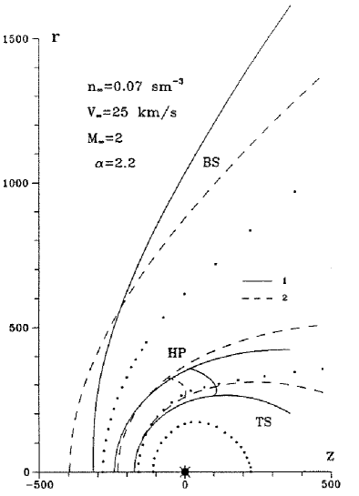
Figure 19: (1) Geometrical pattern of the interface for $\it\alpha=2.2$ [13]. Positions of the bow shock (BS), the termination shock (TS), heliopause (HP), and sonic line in the solar wind. (2) The same lines for $\it\alpha=0$. The discontinuities calculated in [11] in the presence of the neutral hydrogen are shown by dotted lines

It is quite clear from this picture that both the LISM magnetic field and the charge-exchange processes play an important role in the interaction. One can notice that, although a shock-fitting approach perfectly well works in the forward part of the interaction, its limitations reveal themselves in the tail part of the flow. The applicability of the described approach is also limited to axisymmetric problems.

8.4 Shock-capturing calculations

All mentioned in the previous subsection necessitates the application of shock-capturing methods for modeling of the SW–LISM interaction. In [59] this problem was solved in the closed region surrounding an ejecting star on the basis of the flux-splitting method [46]. The choice of parameters was far from those adopted nowadays for the considered problem. Although, as a whole, a physically consistent results were obtained, the resolution of discontinuities was rather poor and some of the obtained data were misinterpreted and disputed in [13].

In [80] the solution of the axisymmetric problem (the LISM magnetic field strength vector is assumed to be parallel to its velocity vector) is presented for realistic SW and LISM parameters. The numerical method applied was developed by Pogorelov [14] and is the high-resolution second-order of accuracy version of the Lax–Friedrichs scheme. This method gives a drastic simplification of the numerical algorithm comparing with the methods based on the exact characteristic splitting of the Jacobian matrices in the MHD equations. Simple but very effective numerical boundary conditions at the far-field were suggested (see Section 2), which allowed one to avoid the influence of spurious reflections from the subsonic outer boundary. An effective procedure of satisfying the condition of source-free magnetic fields (divergence-free condition) was used, which is related to the approach [83].

The formulation of the problem was given is Section 2. Following [14], the numerical flux at the radial cell interface (27) was calculated by the formula

$$\it\displaystyle{\bar{\bf E}}_{l+1/2,n}=\frac{1}{2}\left[{\bar{\bf E}}\left({\bf U}^{R}_{l+1/2,n}\right)+{\bar{\bf E}}\left({\bf U}^{L}_{l+1/2,n}\right)+{\bf\mathchar 8\relax}_{l+1/2,n}\right]\,,$$

(46)

$$\it\displaystyle{\bf\mathchar 8\relax}_{l+1/2,n}=-{\bf{\hat{R}}}_{l+1/2,n}\left({\bf U}^{R}_{l+1/2,n}-{\bf U}^{L}_{l+1/2,n}\right)$$

Here $\it{\bf{\hat{R}}}_{l+1/2,n}$ is the diagonal matrix with the same elements on its diagonal equal to the spectral radius r (the maximum of eigenvalue magnitudes) of the Jacobian matrix $\it{\partial{\bar{\bf E}}\over\partial{\bf U}}$:

$$\it\displaystyle r=|U|+a_{f},\quad a_{f}^{2}={1\over 2}\left((a^{*})^{2}+\sqrt{(a^{*})^{4}-4a^{2}b_{R}^{2}}\right)\,,$$

$$\it\displaystyle b_{R}=B_{R}/(4\pi\rho)^{1/2},\quad B^{2}=B_{R}^{2}+B_{\theta}^{2}\,,$$

$$\it\displaystyle(a^{*})^{2}=(\gamma p+{B^{2}/4\pi})/\rho,\quad a^{2}=\gamma p/\rho\,,$$

where $\it U$ is the radial velocity component and $\it B_{R}$ and $\it B_{\theta}$ are the radial and the angular component of the magnetic field strength vector. Similar formulas can be written for the fluxes in the angular direction.

Having the second order of accuracy, the proposed scheme is much less dissipative than the original Lax–Friedrichs method and provides incomparably better shock resolution. Calculations were performed in the polar computational region with $\it R_{\rm min}=24$ and $\it R_{\rm max}=1200$. The mesh was $\it R\times\theta=99\times 116$.

Mathematically, if we choose the initial distribution of parameters with $\it\mathop{\rm div}\nolimits{\bf B}=0$, the Maxwell equations will preserve this value in the steady solution. In fact, for problems solved numerically the regions of $\it\mathop{\rm div}\nolimits{\bf B}\neq 0$ can be accumulated, especially in the vicinity of discontinuities, see [19]. It is quite clear that the application of the one-dimensional Riemann problem solvers, implying that the component $\it B_{n}$ of the magnetic field vector normal to the boundary is constant, contradicts to the condition $\it\oint B_{n}d\sigma=0$ over the whole computational cell. In [83] an approximate Riemann problem solver for MHD equations was proposed on the basis of the modified system (35) which is conservative only in a steady state. Using the Lax–Friedrichs-type scheme, we do not need such modification, since we do not solve the Riemann problem to find the fluxes at the cell surfaces. The correction in our case can be made by adding to the source term of Eq. (2) the value proportional to $\it\mathop{\rm div}\nolimits{\bf B}$:

$$\it\it{\bf H}^{\prime}=\mathop{\rm div}\nolimits{\bf B}\,\left[0,\,{B_{x}\over 4\pi},\,{B_{z}\over 4\pi},\,{{\bf v}\cdot{\bf B}\over 4\pi},\,u,\,w\right]^{\rm T}$$

This term acts to annihilate the error accumulated if system is solved in the conservation-law form (see [19]). It is worth noting that this approach lies in the framework of Powell’s procedure and the correction term is not small only in the regions of comparably large errors in $\it\mathop{\rm div}\nolimits{\bf B}$. This term, in fact, is equal by the value and opposite by the sign to the appropriate terms proportional to $\it\mathop{\rm div}\nolimits{\bf B}$ appearing by differentiating $\it\bf E$ and G in Eq. (1). The divergence of magnetic field strength vector can be approximated over the finite volumes as

$$\it\displaystyle\mathop{\rm div}\nolimits{\bf B}=[R^{2}_{l+1/2}(B_{n})_{l+1/2,n}+R^{2}_{l-1/2}(B_{n})_{l-1/2,n}]/R^{2}_{l}\mathchar 1\relax R+{}$$

$$\it\displaystyle[(B_{n})_{l,n+1/2}\sin\theta_{n+1/2}+(B_{n})_{l,n-1/2}\sin\theta_{n-1/2}]/R_{l}\sin\theta_{n}\mathchar 1\relax\theta$$

This simple procedure gives a powerful tool for the realization of the divergence-free condition and necessitates only a slight modification of the existing codes for solving MHD equations. It seems limited, however, only to steady-state calculations.

Numerical results were obtained for the same flow parameters as in the previous subsection and for the three different values of the Alfvén number: $\it A=10,\,2,\,\sqrt{2}$. The first value corresponds to the very small magnetic field (see Fig. 20) and can be used for comparison with purely gasdynamic results in which the Roe-type Riemann problem solver was used to obtain the steady state solution, see Subsection 3.2. In Fig. 20, the pressure (below the symmetry axis) and the density logarithm isolines are presented ($\it A=10$). All features of the flow pattern (see Fig. 2) are sharply resolved, while the low time-consumption and the simplicity of the algorithm are quite clear. In Fig. 21 the same distributions are shown for the case $\it A=2$.

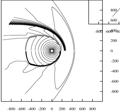
Figure 20: Pressure (below the symmetry axis) and density logarithm isolines, $\it A=10$

In Figs. 22–23, the case with $\it A=\sqrt{2}$ is presented, which corresponds to $\it p_{\rm magn}/p_{\rm thermal}\approx 1.67$ at infinity, that is, $\it B_{\infty}\approx 2.5$ (dimensional value $\it\sim 2.3\times 10^{-6}$ Gauss). In Fig. 23, the streamlines (lower half) and the magnetic field lines are shown.

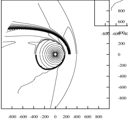
Figure 21: Pressure (below the symmetry axis) and density logarithm isolines, $\it A=2$

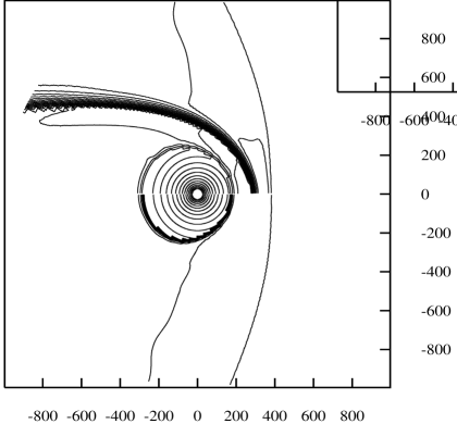
Figure 22: Pressure (below the symmetry axis) and density logarithm isolines, $\it A=1.414$

Figure 23: Streamlines (below the symmetry axis) and magnetic field lines,  $\it A=1.414$.

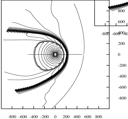
Figure 24: Density logarithm isolines in the symmetry plane

Near the symmetry axis the heliocentric distance of the heliopause increases due to the magnetic field tension, whereas it decreases at the side parts due to the magnetic pressure. On the other hand, although the magnetic field is absent in the region inside the heliopause, its action is revealed by the increased value of the total pressure at infinity. This leads to substantial decrease of the termination shock stand-off distance in the downstream region. We can see the absence of the Mach disk structure in the backward direction. This means that the velocity along the termination shock becomes subsonic. The same occurs if the charge-exchange is taken into account [11]. The bow shock stand-off distance along the symmetry axis becomes smaller than in the absence of magnetic field.

As the magnetic field increases, the effective Mach number, generally speaking, diminishes. The similar effect is produced by the presence of neutral hydrogen atoms and, if both of these factors exceed a definite value, the bow shock can disappear. In this case system (2) becomes elliptic and other methods must be applied for its solution. It is worth noting, however, that the speed of propagation of magnetosonic waves depends on the direction with respect to the magnetic field vector. That means that the effective Mach number varies along the bow shock. As will be shown later, this results in a highly asymmetric shape of the bow shock if magnetic field is not parallel to the velocity vector.

If the magnetic field strength at infinity is equal to its probable upper limit of $\it 3\times 10^{-6}$ Gauss, the LISM flow becomes subsonic, even if the charge-exchange processes are neglected. This can be seen from the simple estimate. We can calculate the LISM effective Mach number as $\it M^{2}_{\rm eff}=\rho_{\infty}V^{2}_{\infty}/(\gamma p_{\infty}+B^{2}_{\infty}/4\pi)$ (this holds, e. g., at the symmetry axis for $\it{\bf V}_{\infty}\perp{\bf B}_{\infty}$ . Thus,$\it 1/M^{2}_{\rm eff}=1/M^{2}_{\infty}+1/A^{2}$ and for $\it M^{2}_{\infty}=4$ the effective Mach number remains larger than unity only for $\it A>1.15$. Thus, both effects are of great importance for the interpretation of data obtained in the space experiment. The performance of the algorithm for the realization of the magnetic field source-free condition can be seen from Fig. 23. The magnetic field lines remain parallel to the streamlines. One can see that no magnetic field penetrates into the heliosphere. This result can not be achieved without a special treatment of the divergence-free condition.

The result of the magnetic field influence on the whole structure of the flow is not sufficiently investigated. It is clear that the flow pattern for $\it{\bf B}_{\infty}\not\parallel{\bf V}_{\infty}$ is three-dimensional. MHD modeling of the heliopause shape on the basis of the Newtonian approximation was performed in [34]. The results of the three-dimensional modeling of the solar wind interaction with the magnetized interstellar medium were presented in [81].

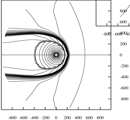
Figure 25: Density logarithm isolines in the plane $\it\varphi=90^{\circ}-270^{\circ}$

Calculations were performed in the spherical computational region with $\it R_{\rm min}=24$ and $\it R_{\rm max}=1200$. The mesh is $\it R\times\theta\times\varphi=99\times 116\times 21$. All parameters are the same as in the previously described axisymmetric calculation and $\it A=2$. In Figs. 24–25 the logarithm density isolines are shown for the case of the angle between $\it{\bf v}_{\infty}$ and $\it{\bf B}_{\infty}$ equal to $\it\alpha=45^{\circ}$ in the cross-sections $\it\varphi=0\hbox{--}180^{\circ}$ and $\it 90^{\circ}\hbox{--}270^{\circ}$, respectively. The LISM influences in this case the shape of the bow shock as well as the location of the stagnation point at the heliopause surface in a way consistent with the simplified study [34]. In addition, the results show the existence of magnetosheath current layers providing proper rotation of the magnetic field with respect to the velocity vector from $\it 45^{\circ}$ to 0 or $\it 180^{\circ}$ at the heliopause surface. The bow shock wave stand-off distance is larger in the regions with a larger angle between the magnetic field and the shock normal. The contact surface is substantially contracted by the magnetic pressure in the $\it xy$-plane (Fig. 25) rather than in the symmetry $\it xz$-plane (Fig. 24). As was mentioned earlier, the size of the zone between the bow shock and the heliopause is very important in view of the charge-exchange processes in this zone.

9 Conclusions

In this work we presented a review of the application of numerical methods to modeling of the stellar wind interaction with the interstellar medium. This is only one among various domains of their application to space simulation problems. The environment of distant stars is not so well investigated as the solar system. That is a particular reason of an extremely intensive study of the solar wind and the local interstellar medium interaction. The problem is rather complicated even in gasdynamic and MHD formulations, since the flow pattern contains a number of intersecting discontinuities and is substantially three-dimensional. The study of this and other astrophysical and industrial problems has recently summoned the extension of high-resolution numerical methods to magnetohydrodynamic flows. The peculiarity of the problem considered in this paper is that a continuum approach is applicable only to the plasma component of the both flows. Trajectories of neutral particles must be calculated using a direct Monte-Carlo simulation. Although several authors (see brief discussion in [110]) argue that the application of a fluid approximation neutrals gives results close to those obtained on the basis of the self-consistent Euler–Boltzmann formulation, there is still a necessity to realize this possibility and to perform a critical comparison of numerical data for the same set of defining parameters.

The influence of the cosmic rays on the interaction is rather well known, but their inclusion into available numerical algorithms is at the initial stage.

We examined in this review mainly numerical aspects of the problem. This work by no means can be considered as an exhaustive description of physical phenomena which take place in the interaction region. Discussing the subject, we inevitably had our preferences and paid them more attention. The list of references can be extended by hundreds of publications on the considered problem, but we hope that even those mentioned in this review give an opportunity to realize the main processes defining the problem and approaches to their numerical modeling.

References

- 1 G.D. van Albada, B. van Leer B., and W.W. Roberts, Astron. & Astrophys., 108, 76 (1982)
- 2 H.Alfvén, Cosmic Electrodynamics, Clarendon Press, Oxford, 1950
- 3 W.I. Axford, Solar Wind, NASA SP-308, 609 (1972)
- 4 K.I. Babenko and V.V. Rusanov, Proc. 2nd U.S.S.R. Meeting on Theoretical Mechanics. Review papers. 2. Nauka, Moscow, 1965
- 5 V.B. Baranov, K.V. Krasnobaev, and A.G. Kulikovskii, Doklady AN SSSR, 194, 41 (1970) [transl. into English as Soviet Physics Doklady]
- 6 V.B. Baranov and K.V. Krasnobaev, Hydrodynamic Theory of Cosmic Plasma, Nauka, Moscow, 1977 [in Russian]
- 7 V.B. Baranov, M.G. Lebedev, and M.S. Ruderman, Astrophys. and Space Sci., 66, 441 (1979)
- 8 V.B. Baranov, M.K. Ermakov, and M.G. Lebedev, Fluid Dynamics, No. 5, 754 (1982)
- 9 V.B Baranov, Interaction of the solar wind with the external plasma, in: Physics of the Outer Heliosphere, Pergamon, New York, 287 (1990)
- 10 V.B. Baranov, M.G. Lebedev, and Yu.G. Malama, Astrophys. J., 375, 347 (1991)
- 11 V.B. Baranov and Yu.G. Malama, J. Geophys. Res., 98, 15157 (1993)
- 12 V.B. Baranov and Yu.G. Malama, J. Geophys. Res., 100, 14755 (1995)
- 13 V.B. Baranov and N.A. Zaitsev, Astron. and Astrophys., 304, 631 (1995)
- 14 A.A. Barmin, A.G. Kulikovskiy, and N.V. Pogorelov, J. Comput. Phys. 126, 77 (1996)
- 15 A. Barnes, J. Geophys. Res., 98, 15137 (1993)
- 16 A. Barnes, J. Geophys. Res., 99, No. A4, 6553 (1994)
- 17 A. Barnes, Space Sci. Rev., 72, 233 (1995)
- 18 P.W. Blum and H.J. Fahr, Nature, 223, 936 (1969)
- 19 J.U. Brackbill and D.C. Barnes, J. Comput. Phys., 35, 326 (1980)
- 20 J.U. Brackbill, J. Comput. Phys., 96, 163 (1991)
- 21 J.C. Brandt, Introduction to the Solar Wind, W.H. Freeman, New York, 1970
- 22 M. Brio and C.C. Wu, J. Comput. Phys., 75, 400 (1988)
- 23 P. Cargo and G. Gallice, ZAMM Special Issue I. Numerical Analysis, Scientific Computing, Computer Science, 369 (1996)
- 24 S. Chakravarthy and S. Osher, AIAA J., 21, 1241 (1983)
- 25 P. Colella and P.R. Woodward, J. Comput. Phys., 54, 174 (1984)
- 26 W. Dai and P.R. Woodward, J. Comput. Phys., 111, 354, (1994).
- 27 W. Dai and P.R. Woodward, J. Comput. Phys., 115, 485, (1994).
- 28 L.E. Davis, Jr., Phys. Rev., 100, 1440 (1955)
- 29 A.J. Dessler, Rev. Geophys., 5, 1 (1967)
- 30 C.R. DeVore, J. Comput. Phys., 92 142 (1991)
- 31 M. Dryer, A.W. Rizzi, and W.-W. Shen, Astrophys. and Space Sci., 22, 329 (1973)
- 32 H.J. Fahr, Solar Physics, 30, 193 (1973)
- 33 H.J. Fahr, Adv. Space Res., 6, 13 (1986)
- 34 H.J. Fahr, et al., Annales Geophysicae, 6, 337 (1988)
- 35 H.J. Fahr, H. Fichtner, and S.Grzedzielski, Solar Physics, 137, 355 (1992)
- 36 P.J. Finley, J. Fluid Mech., 26, 337 (1966)
- 37 D. Givoli, J. Comput. Phys., 94, 1 (1991)
- 38 S.K. Godunov, Mat. Sbornik, 47, 271 (1957) [in Russian] Transl. US Joint Publ. Res. Service, JPRS 7226 (1969)
- 39 T.I. Gombosi, et al., J. Geophys. Res., 101, No. A7, 15233 (1996)
- 40 S. Grzedzielski and R. Ratkiewicz, Acta Astron., 25, 177 (1975)
- 41 T. Hanawa, Y. Nakajima, and K. Kobuta, Dept. of Astrophysics Nagoya University Preprint No. 94–34 (1994).
- 42 Ch. Hirsch, Numerical Computation of External and Internal Flows, John Wiley & Sons, Chichester, 1990
- 43 M.A. Il’gamov, Nonreflecting boundary conditions on the calculation domain boundaries, in: Dynamics of Shells in Flows, Publ. 4-75, Kazanskii Fiz.-Tekh. Inst KF Akad. Nauk S.S.S.R., Kazan, 1985 [in Russian]
- 44 M.A. Il’gamov, Review of research on nonreflecting conditions on the boundaries of the calculational domain, in: Numerical Boundary Conditions, Publ. 6-54, Kazanskii Fiz.-Tekh. Inst KF Akad. Nauk S.S.S.R., Kazan, 1990 [in Russian]
- 45 A. Jeffrey and T. Taniuti, Nonlinear Wave Propagation, Academic Press, New York, 1964.
- 46 T. Jyounouchi, N. Tsujimura, and M. Yasuhara, in: Proc. 4th International Conference in Computational Fluid Dynamics, Nagoya, 964 (1989)
- 47 S.R. Karmesin, P.C. Liewer, and J.U. Brackbill, Geophys. Res. Lett., 22, 1153 (1995)
- 48 I.K. Khabibrakhmanov and D. Summers, J. Geophys. Res., 101, 7609 (1996)
- 49 A. Kulikovskiy and G. Lyubimov, Magneto-hydrodynamics, Addison–Wesley, Reading, MA, 1965.
- 50 R. Lallemant, et al., Astrophys. J., 396, 696 (1992)
- 51 L.D. Landau and E. Lifshits, Electrodynamics of Continuous Media, Pergamon, New York, 1960
- 52 P.C. Liewer, S.R. Karmesin, and J.U. Brackbill, J. Geophys. Res., 101, 17119 (1996)
- 53 R.W. MacCormack, AIAA Paper 81-0110 (1981)
- 54 Yu.G. Malama, Astrophys. Space Sci., 176, 21 (1991)
- 55 T. Matsuda, et al., Progr. Theor. Phys., 81, 810 (1989)
- 56 T. Matsuda, et al., Progr. Theor. Phys., 84, 837 (1990)
- 57 T. Matsuda, et al., Progr. Theor. Phys., 84, 856 (1990)
- 58 T. Matsuda, et al., CFD J., 1, No. 2, 115 (1992)
- 59 T. Matsuda and Y. Fujimoto, in: Proc. 5th Int. Symp. on Comput. Fluid Dyn., Sendai, August 31 – September 3, 1993, 2, 186 (1993)
- 60 G. Moretti, Computers and Fluids, 7, 191 (1979)
- 61 G. Moretti and L. Zanetti, AIAA J., 22, 758 (1984)
- 62 G. Moretti, Computers and Fluids, 15, 59 (1987)
- 63 K. Naidu and A. Barnes, J. Geophys. Res., 99, No. A6, 11553 (1994)
- 64 M. Napolitano and A. Dadone, AIAA J., 23, 1343 (1985)
- 65 M.L. Norman, et. al., Astron. & Astrophys., 113, 285 (1982)
- 66 M.L. Norman, K.-H.A. Winkler, and L. Smarr, in: Atrophysical Jets (eds. A. Ferrari and A.G. Pacholczyk), D. Reidel, 227 (1982)
- 67 S. Nozawa and H. Washimi, Publ. Astron. Soc. Japan, 49, No. 3 (1997)
- 68 T. Ogino, J. Geophys. Res., 91, No. A6, 6791 (1986)
- 69 E.N. Parker, Astrophys. J., 134, 20 (1961)
- 70 H.L. Pauls, G.P. Zank, and L.L. Williams, J. Geophys. Res., 100, No. A11, 21595 (1995)
- 71 H.L. Pauls and G.P. Zank, J. Geophys. Res., 101, 17081 (1996)
- 72 J.L Phillips, et al., Science, 268, 1030 (1995)
- 73 J.L Phillips, et al., in: Solar Wind, 8, in press (1996)
- 74 N.V. Pogorelov and Yu.D. Shevelev, U.S.S.R. Comput. Math. Math. Phys., 25, 1391 (1985)
- 75 N.V. Pogorelov, in: Proc. 5th Int. Symp. on Comput. Fluid Dyn., Sendai, August 31 – September 3, 1993, 3, 7 (1993) [see also CFD J., 6, No. 2, 213 (1997)]
- 76 N.V. Pogorelov, Astron. and Astrophys., 297, 835 (1995)
- 77 N.V. Pogorelov, A.A. Barmin, A.G. Kulikovskiy, and A.Yu. Semenov, Collection of Papers, 6th International Conference on Computational Fluid Dynamics (Lake Tahoe, September 5–9, 1995), 2, 952, University of California, Davis, 1995.
- 78 N.V. Pogorelov and A.Yu. Semenov, Comput. Math. Math. Phys., 36, No. 3, 395 (1996) [translated from Zh. Vychisl. Mat. Mat. Fiz.]
- 79 N.V. Pogorelov and A.Yu. Semenov, in: Numerical Methods in Engineering, John Wiley & Sons, Chichester, 1022 (1996)
- 80 N.V. Pogorelov and A.Yu. Semenov, Astron. and Astrophys., 321, 330 (1997)
- 81 N.V. Pogorelov and T. Matsuda, in: Proc. 5th Int. School/Symposium for Space Simulations, March 13–19, Kyoto, 1997 (1997) [J. Geophys. Res., in press (1997)]
- 82 N.V. Pogorelov and A.Yu. Semenov, Comp. Math. Math. Phys., 37, 320 (1997)
- 83 K.G. Powell, Report NM-R9407, Centrum voor Wiskunde en Informatica, Amsterdam (1994)
- 84 Powell K.G., et al., in: Proc. AIAA 12 Comput. Fluid Dyn. Meeting (1995)
- 85 T.H. Pulliam, AIAA Paper 85-0438 (1985)
- 86 Yu.B. Radvogin, Preprint No. 8, Keldysh Inst. Appl. Math., Moscow, 1987 [in Russian]
- 87 H. Ripken and H.J. Fahr, Astron. & Astrophys., 122, 121 (1983)
- 88 P.L. Roe, J. Comput. Phys., 43, 357 (1981)
- 89 P.L. Roe, Characteristic-based Schemes for the Euler equations, in: Ann. Rev. Fluid Mech., 18, 337 (1986)
- 90 D.J. Romeo and J.R. Sterrett, NASA TN D-1605 (1963)
- 91 D.J. Romeo and J.R. Sterrett, AIAA J. 3, 544 (1965)
- 92 K. Sawada, E. Shima, T. Matsuda, and T. Inaguchi, Mem. Fac. Engg. Kyoto Univ., 48, 240 (1986)
- 93 E.Shima, T. Matsuda, and T. Inaguchi, Monthly Notices Royal Astron. Soc., 221, 687 (1986)
- 94 L. Smarr, M.L. Norman, and K.-H.A. Winkler, Phisica, 12D, 83 (1984)
- 95 J.R. Spreiter, A.L. Summers, and A.W. Rizzi, Planet. Space Sci., 18, 1281 (1970)
- 96 R.S. Steinolfson, V.J. Pizzo, and T. Holzer, Geophys. Res. Lett., 21, No. 4, 245 (1994)
- 97 R.S. Steinolfson, J. Geophys. Res., 99, No. A7, 13307 (1994)
- 98 J.L. Stone and M.L. Norman, Astrophys. J. Suppl., 80, 753 (1992)
- 99 S.T. Suess, D.H. Hathaway, and A.J. Dessler, Geophys. Res. Lett., 14, No. 9, 977 (1987)
- 100 S.T. Suess, J. Geophys. Res., 98, No. A9, 15147 (1993)
- 101 M.T. Sun, S.T. Wu, and M. Dryer, J. Comput. Phys., 116, 330 (1995)
- 102 K.W. Thompson, J. Comput. Phys., 68, 1 (1987)
- 103 G. Tóth and D. Odstrĉil, J. Comput. Phys., 128, 82 (1996)
- 104 M.K. Wallis, Nature Phys. Sci., 233, 23 (1971)
- 105 M.K. Wallis, Nature, 254, 202 (1975)
- 106 M.K. Wallis and M. Dryer, Astrophys. J., 205, 895 (1976)
- 107 H. Washimi, Adv. Space Res., 13, No. 6, 227 (1993)
- 108 H. Washimi and T. Tanaka, Space Sci. Rev., 78, 85 (1996)
- 109 K. Watanabe and T. Sato, J. Geophys. Res., 95, No. A1, 75 (1990)
- 110 L.L. Williams, D.T. Hall, H.L. Pauls, and G.P. Zank, Astrophys. J., 476, 366 (1997)
- 111 C.C. Wu and C.F. Kennel, Geophys. Res. Lett., 19, 2087 (1992)
- 112 H.C. Yee, NASA TM-101088 (1989)
- 113 N.A. Zaitsev and Yu.B. Radvogin, Preprint No. 86, Keldysh Inst. Appl. Math., Moscow, 1990 [in Russian]
- 114 A.L. Zachary and P. Colella, J. Comput. Phys., 99, 341, (1992)
- 115 G.P. Zank, H.L. Pauls, L.L. Williams, and D.T. Hall, J. Geophys. Res., 101, No. A10, 21639 (1996)