CAVITY LOSS FACTORS FOR NON-ULTRARELATIVISTIC BEAMS

Abstract

Cavity loss factors can be easily computed for ultrarelativistic beams using time-domain codes like MAFIA or ABCI. However, for non-ultrarelativistic beams the problem is more complicated because of difficulties with its numerical formulation in the time domain. We calculate the loss factors of a non-ultrarelativistic bunch and compare results with the relativistic case.

1 Introduction

It is common to believe that loss factors of a bunch moving along an accelerator structure at velocity $v=\beta c$ with $\beta<1$ are lower than those for the same bunch in the ultrarelativistic case, $\beta\to 1$. The loss factors are then computed numerically for the ultrarelativistic bunch, which is a relatively straightforward task, and considered as upper estimates for the case in question, $\beta<1$.

We study $\beta$-dependence of loss factors in an attempt to develop a method to obtain answers for $\beta<1$ case from the results for $\beta=1$. It is demonstrated that the above assumption on the upper estimate might be incorrect in some cases, depending on the bunch length and properties of the structure (cavity + pipe) under consideration.

2 Beam Coupling Impedance and Loss Factors of a Cavity

In the frequency domain and in the ”closed-cavity” approximation (which means very narrow beam pipes) the beam coupling impedance calculation can be reduced to an internal eigenvalue boundary problem. Let $\vec{E}_{s}$, $\vec{H}_{s}$ be a complete set of eigenfunctions (EFs) for the boundary problem in a closed cavity with perfect walls. The longitudinal impedance is then given by (e.g., [1])

$$Z(\beta,\omega)=-i\omega\sum_{s}{{1}\over{\omega^{2}_{s}-\omega^{2}}}{{|I_{s}(\beta,\omega)|^{2}}\over{2W_{s}}}\,,$$ (1)

where $I_{s}(\beta,\omega)=\int_{L}{dz\exp(-i\omega z/\beta c)E_{sz}(0,z)}$ is the overlap integral, and $W_{s}$ is the energy stored in the $s$-th mode. Here $E_{sz}(0,z)$ is the longitudinal component of the $s$-th mode electric field taken on the chamber axis.

There is a resonant enhancement of the $s$-th term in the series (1) for $Z(\beta,\omega)$ as $\omega\to\omega_{s}$. Let us introduce a finite, but small absorption into the cavity walls by adding an imaginary part to the eigenvalue: $\omega_{s}\to\omega^{\prime}_{s}-i\omega^{\prime\prime}_{s}=\omega^{\prime}_{s}(1-i/2Q_{s})$. Here the Q-value of the $s$-th mode is $Q_{s}=\omega^{\prime}_{s}W_{s}/P_{s}\gg 1$, where $P_{s}$ is the averaged power dissipated in the cavity walls ( plus, in a real structure, due to radiation into beam pipes). For $\omega\simeq\omega^{\prime}_{s}$ the $s$-th term in Eq. (1) dominates:

$$Z(\omega\simeq\omega^{\prime}_{s})\simeq R_{s}(\beta)={Q_{s}\over 2\omega^{\prime}_{s}W_{s}}|I_{s}(\beta,\omega^{\prime}_{s})|^{2}\,.$$ (2)

The quantity $R_{s}(\beta)$ is the shunt impedance of the $s$-th cavity mode, and, unlike the $Q$-factor, it depends on $\beta$.

The beam loss factor is

$$k=\frac{1}{\pi}\int_{0}^{\infty}d\omega\ Re\,Z(\beta,\omega)|\lambda(\omega)|^{2}\ ,$$ (3)

where $\lambda(\omega)=\int ds\exp{[i\omega s/(\beta c)]}\lambda(s)$ is a harmonic of bunch spectrum. For a Gaussian bunch with rms length $2l$, the line density is $\lambda(s)=\exp{(-s^{2}/2l^{2})}/(\sqrt{2\pi}l)$ and $\lambda(\omega)=\exp\{-[\omega l/(\beta c)]^{2}/2)\}$. Assuming all $Q_{s}>>1$ and integrating formally Eq. (1) for the $Re\,Z(\beta,\omega)$, one can express the loss factor as a series

$$k(\beta,l)=\sum_{s}k_{s}(\beta,l)=\sum_{s}\exp{\left[-\left(\frac{\omega^{\prime}_{s}l}{\beta c}\right)^{2}\right]}\frac{\omega^{\prime}_{s}R_{s}(\beta)}{2Q_{s}}\ ,$$ (4)

where the loss factors of individual modes $k_{s}$ in the last equation are written for the Gaussian bunch.

In principle, Eq. (4) give us the dependence of the loss factor on $\beta$. However, the answer was obtained in the “closed-cavity” approximation. Moreover, it is practical only when the number of strong resonances is reasonably small, since their the $\beta$-dependence varies from one resonance to another:

$$\frac{k_{s}(\beta,l)}{k_{s}(1,l)}=\exp{\left[-\left(\frac{\omega^{\prime}_{s}l}{c}\right)^{2}\frac{1}{\beta^{2}\gamma^{2}}\right]}\frac{R_{s}(\beta)}{R_{s}(1)}\ ,$$ (5)

where $\gamma=1/\sqrt{1-\beta^{2}}$. It is obvious from Eq. (5) that for long bunches loss factors will decrease rapidly with $\beta$ decrease, as $\exp\left(-\beta^{-2}\right)$. Indeed, the lowest resonance frequencies are $\omega^{\prime}_{s}\approx c/d$, where $d$ is a typical transverse size of the cavity. The exponent argument $-(l/d)^{2}$ will have a large negative value for $l\geq d$, and the exponential decrease for small $\beta$ will dominate the impedance ratio. The impedance ratio dependence on $\beta$ is more complicated, and we consider below a few typical examples.

3 Examples

3.1 Cylindrical Pill-Box

For a cylindrical cavity in the limit of a vanishing radius of beam pipes, $b\to 0$, one can obtained explicit expressions of the mode frequencies and impedances, e.g., [1]. Let the cavity length be $L$ and its radius be $d$. The mode index $s=(m,n,p)$ means that there are $m$ radial variations and $p$ longitudinal ones of the mode $E$-field. The resonance frequency is $\omega_{mnp}=\sqrt{\mu^{2}_{mn}+(\pi pd/L)^{2}}c/d$, where $\mu_{mn}$ is the $n$-th zero of the first-kind Bessel function $J_{m}(x)$. The longitudinal shunt impedance is

$$R_{0np}={Z_{0}\over 2\pi\beta^{2}}{L^{3}\over d^{2}\delta}{\mu^{2}_{0n}\over J^{2}_{1}(\mu_{0n})}{c\over\omega_{0np}d}{1\over 1+\delta_{p0}+2d/L}\times$$

$$\times\left[\left({\omega_{0np}L\over 2\beta c}\right)^{2}-\left({\pi p\over 2}\right)^{2}\right]^{-2}\left\{{\sin^{2}\atop\cos^{2}}\right\}\left({\omega_{0np}L\over 2\beta c}\right).$$ (6)

The upper line in {$\ldots$} corresponds to even $p$ and the lower one to odd $p$, and $\delta$ is the skin-depth.

The ratio of loss factors Eq. (5) for the lowest $E$-mode, $E_{010}$, is then

$$\frac{k_{010}(\beta,l)}{k_{010}(1,l)}=\exp{\left[-\left(\frac{\mu_{01}l}{d\beta\gamma}\right)^{2}\right]}\left(\beta\frac{\sin{\frac{\mu_{01}L}{2\beta d}}}{\sin{\frac{\mu_{01}L}{2d}}}\right)^{2}.$$ (7)

Obviously, it is almost independent of $\beta$ when the bunch is short, $l\ll d$, and the cavity is short compared to its radius, $L\ll d$. For longer cavities, however, the ratio oscillates and might exceed 1. This strong resonance behavior is clearly seen in Fig. 1 for large $L/d$, while for small $L/d$ the $k$-ratio slowly decreases with $\beta$ decrease. For some particular parameter values, $k_{010}(\beta)$ can be many times larger than $k_{010}(1)$. A picture for a longer bunch is similar except the resonances at small $\beta$s are damped heavily.

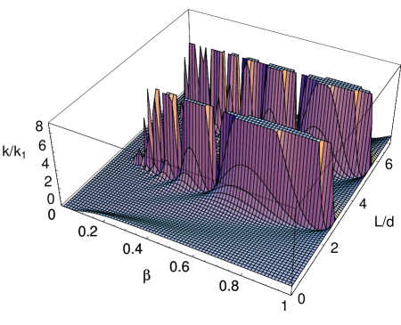
Figure 1: Ratio of loss factors (7) for a short bunch, $l/d=0.05$, versus $\beta$ and resonator length $L/d$.

3.2 APT 1-cell Cavity

As a more realistic example, we consider an APT superconducting (SC) 1-cell cavity with a power coupler [2]. Of course, such a cavity with wide beam pipes to damp higher order modes can not be described completely by the formalism of Sect. 2, except for the modes below the pipe cutoff. Direct time-domain computations with the codes MAFIA [3] and ABCI [4] show the existence of only 2 longitudinal modes below the cutoff for the $\beta=0.64$ cavity, and only 1 for $\beta=0.82$, in both cases including the fundamental mode at $f_{0}=700$ MHz. The loss factor contributions from these lowest resonance modes for a Gaussian bunch with the length $l=3.5$ mm for $\beta=0.64$, and $l=4.5$ mm for $\beta=0.82$, are about 1/3 of the total loss factor.

We use MAFIA results for the field of the lowest mode to calculate the overlap integral and study the loss factor dependence on $\beta$. The on-axis longitudinal field of the fundamental mode is fitted very well by a simple formula $E_{z}(z)=E_{z}(0)\exp{[-(z/a)^{2}]}$, where $a=0.079$ m for $\beta=0.64$ and $a=0.10$ m for $\beta=0.82$, see [5] for detail. The ratio of the shunt impedances in Eq. (5) is then easy to get analytically

$$\frac{R_{s}(\beta)}{R_{s}(1)}=\exp{\left[-\frac{1}{2}\left(\frac{\omega a}{c}\right)^{2}\frac{1}{\beta^{2}\gamma^{2}}\right]}\ ,$$ (8)

where $\omega=2\pi f_{0}$. The resulting dependence shows a smooth decrease at lower $\beta$s. The loss factor for the lowest mode for $\beta=0.64$ is 0.614 times that with $\beta\to 1$, and for $\beta=0.82$ is 0.768 times the corresponding $\beta=1$ result.

3.3 APT Cavity, 5 cells

For 5-cell APT SC cavities the lowest resonances are split into 5 modes which differ by phase advance per cell $\Delta\Phi$, and their frequencies are a few percent apart [2]. We use MAFIA results [6] for these modes to calculate their loss factors according to Eq. (4). The on-axis fields of two modes, with $\Delta\Phi=0$ (0-mode) and $\Delta\Phi=\pi$ ($\pi$-mode), which is the cavity accelerating mode, are shown in Fig. 2.

Figure 2: Longitudinal on-axis electric field (arbitrary units) for 0-mode (dashed) and fundamental ($\pi$-) mode in a half of the 5-cell APT $\beta=0.82$ cavity.

Time-domain simulations with the code ABCI [4] give us the loss factor of a bunch at $\beta=1$. The loss factor spectrum for the $\beta=0.64$ cavity, integrated up to a given frequency, has two sharp steps: one near 700 MHz with the height 0.5 V/pC and the other near 1400 MHz with the height about 0.1 V/pC. They correspond to the two bands of the trapped monopole modes in the cavity, cf. Table 1.

We calculate numerically overlapping integrals in Eq. (4) for a given $\beta$. The results for the loss factors of the lowest monopole modes are presented in Table 1. The totals for the TM₀₁₀ and TM₀₂₀ bands for $\beta=1$ in Table 1 agree very well with the time-domain results. In fact, we are mostly concerned about only these two resonance bands, since the higher modes are above the cutoff, and they propagate out of the cavity into the beam pipes depositing most of their energy there. Our results for the design values of $\beta$ are in agreement with those obtained in [2]. Remarkably, the total loss factors for a given resonance band in Table 1 are lower for the design $\beta$ than at $\beta=1$. The only exception is the TM₀₂₀ band for the $\beta=0.82$ cavity, but it includes some propagating modes, and its contribution is very small.

The $\beta$-dependence of the loss factor for two TM₀₁₀ modes mentioned above (0- and $\pi$-mode) is shown in Fig. 3. Obviously, the shunt impedance (and the loss factor) dependence on $\beta$ is strongly influenced by the mode field pattern.

Table 1: Loss Factors (in V/pC) in APT 5-cell Cavities

$\Delta\Phi$	$f$, MHz	$k(\beta)$	$k(1)$	$k(\beta)/k(1)$
$\beta=0.64$, TM010-band
0	681.6	$7.2\,10^{-6}$	$3.7\,10^{-4}$	0.020
$2\pi/5$	686.5	$4.8\,10^{-5}$	$2.9\,10^{-2}$	0.0016
$3\pi/5$	692.6	$1.1\,10^{-4}$	0.218	0.0005
$4\pi/5$	697.6	$1.2\,10^{-3}$	0.250	0.0049
$\pi$	699.5	0.184	$9.2\,10^{-3}$	19.92
Total		0.185	0.507	0.365
$\beta=0.64$, TM020-band
0	1396.8	$6.5\,10^{-4}$	$5.4\,10^{-4}$	1.187
$2\pi/5$	1410.7	$1.2\,10^{-6}$	$9.0\,10^{-4}$	0.0014
$3\pi/5$	1432.7	$1.8\,10^{-5}$	0.0173	0.0011
$4\pi/5$	1458.8	$8.0\,10^{-7}$	0.0578	$1.4\,10^{-5}$
$\pi$	1481.0	$3.5\,10^{-7}$	0.0095	$3.7\,10^{-5}$
Total		$6.7\,10^{-4}$	0.086	$7.8\,10^{-3}$
$\beta=0.82$, TM010-band
0	674.2	$0.3\,10^{-6}$	$6.9\,10^{-4}$	$4.5\,10^{-4}$
$2\pi/5$	681.2	$7.3\,10^{-5}$	$1.6\,10^{-5}$	4.64
$3\pi/5$	689.9	$1.8\,10^{-6}$	0.034	$5.1\,10^{-5}$
$4\pi/5$	697.2	$1.3\,10^{-3}$	0.220	$5.9\,10^{-3}$
$\pi$	699.9	0.285	$0.240$	1.188
Total		0.286	0.494	0.579
$\beta=0.82$, TM020-band
0	1357.7	$4.2\,10^{-5}$	$0.8\,10^{-6}$	52.4
$2\pi/5$	1367.7	$1.4\,10^{-4}$	$8.0\,10^{-5}$	1.71
$3\pi/5$	1384.5	$1.6\,10^{-6}$	$1.4\,10^{-4}$	0.011
$4\pi/5{}^{*}$	1409.6	$8.0\,10^{-7}$	$1.3\,10^{-3}$	$5.6\,10^{-3}$
$\pi{}^{**}$	1436.9	$1.6\,10^{-2}$	$2.2\,10^{-3}$	7.5
Total		$1.6\,10^{-2}$	$3.7\,10^{-3}$	4.32

^∗Mode near the cutoff.
^∗∗Propagating mode, above the cutoff.

Figure 3: Loss factor ratio vs $\beta$ for 0-mode (dashed) and fundamental ($\pi$-) mode in the 5-cell APT $\beta=0.82$ cavity.

4 Summary

The examples above compare loss factors for $\beta<1$ with $\beta\to 1$ results. More details can be found in [5]. Essentially, the frequency-domain approach has been applied instead of the time-domain one. It can be done only when we know the fields of all modes contributing significantly into the loss factor. Nevertheless, for many practical applications, including SC cavities, the lowest mode contribution is a major concern, because propagating modes travel out of the cavity and deposit their energy away from the structure cold parts.

One interesting observation is that the loss factor of an individual mode at some $\beta<1$ can be many times larger than for $\beta=1$. Obviously, one should exercise caution in using $\beta=1$ results as upper estimates for a $\beta<1$ case.

The author would like to thank Frank Krawczyk for fruitful discussions and for providing MAFIA results for the 5-cell cavities. Useful discussions with Robert Gluckstern and Thomas Wangler are gratefully acknowledged.

References

- [1] S.S. Kurennoy, “Beam-Chamber Coupling Impedance. Calculation Methods”, Phys. Part. Nucl. 24, 380 (1993); also CERN SL/91-31 (AP), Geneva, 1991.
- [2] F.L. Krawczyk, in PAC97, Vancouver, BC (1997); also LA-UR-97-1710, Los Alamos, 1997.
- [3] T. Weiland et al., Proc. 1986 Lin. Acc. Conf., SLAC Report 303, p.282; MAFIA Release 4.00 (CST, Darmstadt, 1997).
- [4] Y.H. Chin, Report LBL-35258, Berkeley, 1994.
- [5] S.S. Kurennoy, Report LA-CP-98-55, Los Alamos, 1998.
- [6] F.L. Krawczyk, private communication, November 1997.