Kinetic Theoretical Foundation of Lorentzian Statistical Mechanics
Abstract
A new kinetic theory Boltzmann-like collision term including correlations is proposed. In equilibrium it yields the one-particle distribution function in the form of a generalised-Lorentzian resembling but not being identical with the so-called distribution frequently found in collisionless turbulent systems like space plasmas. We show that this distribution function satisfies a generalised -theorem, yields an expression for the entropy that is concave. Thus, the distribution is a ‘true’ thermodynamic equilibrium distribution, presumably valid for turbulent systems. In equilibrium it is possible to construct the fundamental thermodynamic quantities. This is done for an ideal gas only. The new kinetic equation can form the basis for obtaining a set of hydrodynamic conservation laws and construction of a generalised transport theory for strongly correlated states of a system.
pacs:
05.20.-y, 05.70.Ce, 51.10.+y, 52.25.Dg, 52.35.Ra, 52.65.Ff, 94.20. RrI Introduction
Statistical mechanics is based on kinetic theory. Classical statistical mechanics derives from Boltzmann’s equation which is the evolution equation for the one-particle phase-space distribution function . The Boltzmann equation itself results from the BBGKY hierarchical correlation expansion of the Liouville equation where the particular collision term is assumed to contain short range interactions only and all orders of correlations are neglected. In kinetic equilibrium the Boltzmann collision term has as solution the celebrated Maxwell-Boltzmann distribution function as the basic distribution function of classical equilibrium statistical mechanics and thermodynamics. These equilibria are characterised by the action of Boltzmann’s -theorem (e.g., [1]) proving that the time evolution of the thermodynamic system tends towards maximum Boltzmannian entropy . Both -theorem and entropy are functionals of the Boltzmann distribution, being the fundamental thermodynamic function. In the past, generalisations of this entropy to quantum statistics of Fermions and Bosons have been very successful. In addition other quantum generalisations have been proposed to fractional statistics of anions by Haldane [2, 3, 4] and others. These generalisations were mostly based on probability counting statistics.
The function has been widely used without justification to even describe collisionless equilibria or as the initial state of the evolution of collisionless systems. Final states of such systems are often described in terms of a perturbation analysis as solutions of a velocity space diffusion process governed by the Fokker-Planck equation for which sometimes it can be demonstrated that a -theorem similar to Boltzmann’s exists as well. Such a situation as in quasilinear theory can be taken as justification for the validity of the perturbation approach. However, in collisionless systems containing strong correlations and consequently exhibiting interactions on all scales typical for strongly turbulent systems and phase transitions the Fokker-Planck perturbation approach may become invalidated. Such systems sometimes cannot be subordinated to Boltzmannian statistical mechanics. Moreover, measurements of velocity space and energy distribution functions in realistic natural systems frequently exhibit properties that are distinctly different from diffusive Fokker-Planck solutions [5, 6, 7]. The observed (classical) distribution functions frequently asymptotically exhibit extended high energy tails of a certain nearly constant slope , with an arbitrary positive real number that is limited from below. Such distributions have been tentatively named distributions and have been used in the past for interpretational purposes [9] as well as for formal derivations [10, 11], investigation of the dispersive properties of -plasmas [12, 13] and calculation of their thermal fluctuation levels [14, 15].
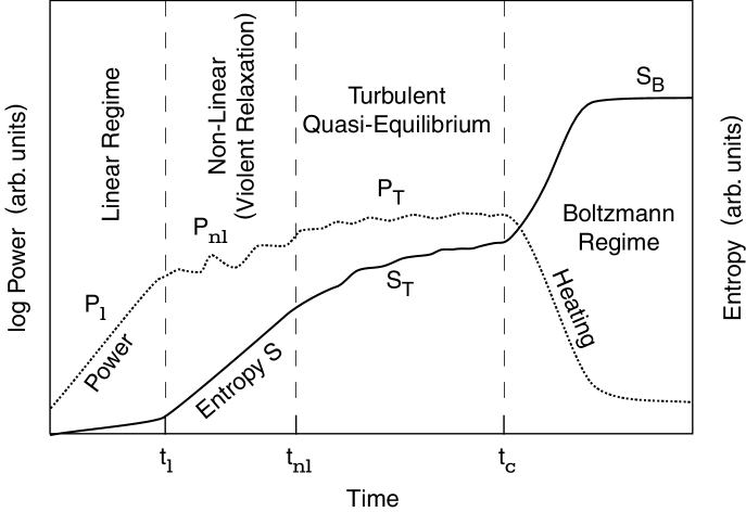
All these facts lead to the question if not in collisionless systems equilibrium states may (possibly temporarily) evolve that are distinctly different from Boltzmann equilibria. In fact, given a system containing some sufficiently large amount of free energy and being nearly collisionless, i.e. having a certain very small collision frequency , the evolution of the system will during its initial state be entirely independent of the presence of collisions between its particle constituents. Instead it will undergo an instability, i.e., the free energy will drive some of the fundamental eigen modes of the system unstable. As a consequence, the amplitudes of these modes will grow from their thermal level until they assume finite values, and the system will evolve into some previously non-existent structure. Since collisions are very rare for times comparable to the linear time , with the linear growth rate, the system behaves initially linearly. The eigen-mode amplitudes grow exponentially until becoming large enough that the linear approximation breaks down. The system then enters into its non-linear state.
Let us assume that this state is quickly reached such that collisions are still unimportant. The further evolution of the system will then be determined by various non-linear effects like wave-wave interactions, wave-particle and non-linear wave-particle interactions, generation of anomalous collisions when the particles are scattered at the waves etc. In short, the system becomes turbulent. The large-amplitude eigen-modes excite sideband waves, local inhomogeneity is introduced, and the system evolves into a state of coexistence of many different mutually interconnected scales affecting each other. The total power in the system will, in this state, start to behave fluctuating, possibly still growing and reorganising the system continuously. Assume the non-linear time still being much shorter than the collision time, . For collisions still being negligible, this state may last for a certain possibly long turbulent time . Such an evolution is sketched in Figure 1.
The intermediate nonlinearly turbulent state represents a thermodynamic quasi-equilibrium state different from the purely stochastic thermodynamic equilibria described by the correlation-free Boltzmann statistical mechanics. Since the state is a quasi-equilibrium state, it should possess an equilibrium distribution function that is different from , and in addition its entropy should be approximately constant such that it assumes an intermediate approximate maximum for the time interval . Clearly, when the final state of the system is approached at time , the system becomes collisional, and binary collisions will destroy the intermediate turbulent quasi-equilibrium. After , stochasticity dominates over the turbulent correlations, and the power contained in the turbulent fluctuations is readily converted into heat. The system then settles at its ultimate thermal equilibrium that is described by ordinary Boltzmann statistical mechanics.
The free parameter introduced above heuristically describes the deviation of the turbulent quasi-equilibrium distribution function from the Boltzmann distribution. It contains the information about the actual turbulent processes and correlations in the system. In the absence of correlations and scale-invariance it will behave in a way that the quasi-equilibrium distribution approaches the Boltzmann distribution. The motiviation for introducing follows the experimental literature and is thus purely traditional. However, as will be shown below, it turns out to be nevertheless practical. In a real turbulent system the entropy will still tend to increase slowly due to weak internal turbulent dissipation processes, but in an approximate theory we may assume that this increase is slow enough for the state to be considered stationary. These assumptions allow to ask for the possible form of the quasi-equilibrium distribution function and for the statistical mechanics of the equilibrium state described by it.
The existence of a non-Boltzmannian statistical mechanics has been suspected since the observation of Lévy flights (for an account of the current literature on this subject cf., e.g., [16]). Lévy flights have been suspected to affect plasma transport and diffusion. The random walks caused by Lévy flights have been shown to possess an approximate distribution function resembling the distribution [17] though no ultimate theory of Lévy flights is available yet. Beginning with Renyi [18, 19] intuitive but formal extensions of Boltzmann’s theory of the statistical entropy have been suggested in order to find different concepts for the entropy as the basic thermodynamic function of a modified statistical mechanics. A whole family of such formal generalisations could be imagined not all of them being of physical relevance. More recently [20] a particular heuristic simplification of Renyi’s entropy has been proposed which seems to deserve some physical applicability but still lacks a basic physical or probabilistic foundation. Among the applications proposed are diffusion [21], hydrodynamic turbulence [22] and others. It has, moreover, been shown that the thermodynamic formalism could be extended to this kind of entropy [22], and the fluctuation-dissipation theorem [23] could be formulated as well. A disadvantage of this theory is that it apparently allows for a violation of the second law when entropic growth seems to be inhibited. Such a behaviour is generally considered to be rather unphysical. Its advantage over Renyi’s original proposal is its formal simplicity.
In this communication we construct the one-particle kinetic equivalent of the Boltzmann equation which forms the physical basis for a generalised-Lorentzian statistical mechanics. We demonstrate that in thermodynamic equilibrium its solution is the real and positive definite generalised-Lorentzian phase space distribution function
| (1) |
where is the (non-relativistic) particle energy, the chemical potential that is related to the fugacity , and is a certain normalisation constant (extension to the relativistic or to non-ideal cases including external force fields is then straightforward). The Lagrangean multiplier is a function of the temperature of the system, which is the physical observable, is a positive real valued but otherwise arbitrary number that can assume any positive value . For , the above distribution smoothly approaches the Boltzmann function .
II The Lorentzian Collision Term
The final step in the BBGKY kinetic theory of solution of the exact Liouville equation for a many particle system is the one-particle kinetic equation for the one particle distribution function
| (2) |
where is the one-particle Liouville (Boltzmann) operator acting in the one-particle phase space. The collision operator on the right-hand side of Equation (2) depends on the one and two-particle distribution functions , respectively, as well as on the particle number . It is a very complicated functional that in principle traces back through the entire hierarchy to the original -particle Liouville equation. In order to arrive at any physically useful solutions it must be approximated in some way. The most widely used approximations are Boltzmann’s hypothesis of statistical independence of the interactions in any kind of collisions and the collisionless assumption of Vlasov. The latter leads to the neglect of the collision term, attributing all interactions to the action of the fields on the one-particle distribution function on the left-hand side of Eq. (2). This assumption is very strong because even in the absence of any binary one-particle collisions, the action of the fields and very weak higher-order collisions on the level of the two-particle equation in the BBGKY hierarchy may result in a non-vanishing one-particle collision term . This term may contain residual correlations and may thus not necessarily be of the correlation-free statistically independent Boltzmann form proposing that is a functional of the product of two one-particle distribution functions only:
| (3) |
The form stands for , where the index designates the number of the particle involved whose position in momentum and configuration space are . Its explicit form is
| (4) |
The prime indicates the particles after the collision, with the collisional cross-section, and the solid angle of the collision. The cross-section depends on the elementary physics of the collision process and has to be determined separately for the individual process in question. In central force fields, it becomes the Boltzmann-Rutherford cross section. For purely field-mediated interactions it is a complicate function. However, in order to determine the distribution function in thermal equilibrium, explicit knowledge of the differential cross-section is not needed. All that is required is that is positiv definite. This holds for any real physical process.
The molecular chaos assumption underlying Boltzmann’s theory refers to the absence of all interactions between the particles other than binary with two-particle correlation function . It thus reduces to to the product of the two one-particle distribution functions . In such an approach the binary interactions dominate on all scales and for all times, an assumption that has turned out very fruitful in classical statistical mechanics. However, as mentioned above, under certain conditions like scale-invariance this assumption may become violated. Self-consistent field fluctuations may lead to long-range correlations in the system and clustering of particles in groups that behave similarly on many different scales. Under such conditions molecular chaos will be replaced by chaos on larger scales that are dominated by correlations among the particles. Clearly, such interactions depend crucially on the particular kind of correlation induced, and the general behaviour of the system becomes very difficult to investigate.
There are two primary effects caused by such correlations. The first is a change in the differential cross-section. More important for our purposes here is the change induced in the two-particle correlation function in the collision integral (4). Without explicit knowledge about the particular turbulent process it seems that little more could be said. However, in a first approach to a statistical theory one may follow Boltzmann’s approach and assume that even in the turbulent regime the one-particle distribution function still satisfied the lowest-order kinetic equation of the BBGKY hierarchy, i.e., Boltzmann’s equation (2), but now with different (turbulent) collision term
| (5) |
that takes into account the correlations via the turbulent so far unspecified correlation functional . In this expression the positive definite turbulent differential cross-section contains the supposed interactions between the clustered groups of particles at different scales formally in the same way as in Boltzmann’s case. The explicit form of the cross-section is not of primary importance for our purposes in the following. Its calculation for particular cases will be delayed to elsewhere. Its nature to be a collisional cross section guaranties its positive definiteness. This is all we need here in developing an equilibrium theory.
The turbulent conglomerates behave like superparticles. If this is the case, one can model the two-particle correlation function as the uncorrelated product of functionals of the one-particle distribution function tentatively describing the approximately uncorrelated interaction of the superparticles formed by the long range correlation of the particles in the system. The underlying assumption in this approach is that the long-range correlations become very weak on a sufficiently large scale such that the molecular chaos assumption holds again if the scale is chosen sufficiently large. In other words, the assumed scale-invariance must be broken at sufficiently large scales. This is certainly a valid assumption for most physical systems. Then we can write
| (6) |
In accord with the previous discussion, higher order correlations are neglected in this representation. The so far unspecified mechanism of how the cluster conglomerates and congregates are formed and which part of the phase space is occupied by each of them is thereby buried in the particular functional form of .
III Correlation Functional and Equilibrium Distribution
Our primary task is to find an analytic expression for the functional . Clearly, any rigorous theory should derive from the Liouville equation or at least from the kinetic equation for the two-particle correlation function , i.e. from the second-lowest order equation in the BBGKY hierarchy. Here we follow a more heuristic elementary approach.
Let us assume homogeneous force-free equilibrium conditions such that . The Boltzmann equation then requires that the collision term (5) vanishes identically. A sufficient condition for this to happen is that the correlation functional
| (7) |
This requirement does not depend on the explicit form of the differential cross section as long as the latter is positive definite, as we have assumed. It is thus a very general assumption holding for any equilibrium theory. Taking the logarithm of yields
| (8) |
This expression corresponds to Boltzmann’s equilibrium condition with the only difference that it is now demanded to be satisfied by the functionals instead of the distribution function itself. However, because the underlying interaction between the particles remains to be deterministic, must be a function of the constants of motion only, viz. particle number and energy. Thus the general solution to the above equation is
| (9) |
where are two arbitrary real constants, and is the initial average momentum of the particles of mass that they may have possessed in common. The constant somehow takes care of the conservation of the particle number. In addition we introduced the free parameter on that may also depend, playing the role of a control parameter that characterises the particular nature of the correlations caused by the specific long range processes in the medium. The functional hereby turns out to be an exponential function of the particle energy. In order to find its functional dependence on , it should be inverted for . This is not possible without any further assumptions. One of these assumptions can be based on our additional knowledge that in the limit of molecular chaos the Boltzmannian statistical mechanics must be recovered. We, hence, liberately demand that in the limit the functional should become the identity functional
| (10) |
This requirement can be taken as a guideline in the search for the functional form of .
Let us assume that the one-particle distribution function has been normalized to one. This assumption is easy to satisfy for any given distribution function since the physical interpretation of the distributions is to be a probability distribution function. The simplest possible function that satisfies the above condition is
| (11) |
where we dropped the index 1 for simplicity, since from now on we will understand as the one-particle distribution function. It is easy to check that (11) actually becomes the identity functional for the free parameter . There may be other functional forms as well which satisfy (10). However, in view of the free parameter , Eq. (11) is the simplest choice one can make.
In order to find the equilibrium distribution function , we invert Equation (11) and combine the result with Equation (9). This procedure yields
| (12) |
where takes care of the proper normalisation of the distribution function. Taking the limit one again easily checks that , and this distribution becomes the Boltzmann function in the large- limit. Hence, from (12) solves the equilibrium one-particle kinetic equation (2) with the new collision term (5) including turbulent correlations.
The new distribution function is a -generalised Lorentzian function similar to those particle distributions that have been measured in space plasmas [5, 6]. It may also apply to Lévy flight statistics. It contains three free parameters, and . The limit suggests that can be identified with the kinetic temperature of the system under consideration, while the so far unspecified free parameter is the chemical potential. For this chemical potential itself becomes a function of . Moreover, for finite , unlike the Boltzmann case, it does not drop out of the distribution function but is retained suggesting that finite- systems do not behave like normal statistical systems but possess an internal chemical potential that affects the addition or extraction of particles.
Before proceeding to the next sections where we prove that the above distribution function describes a real thermodynamic equilibrium, we note that the free parameter necessarily satisfies a number of restrictions imposed on it by the requirement that the equilibrium distribution function must conserve the particle number and average energy of the particles in the system. A naive inspection of (12) may suggests that . Below we will show that actually for an ideal gas, which is a much stronger restriction on . We also note once more that implicitly contains all information about the real turbulent dynamics of the system. Calculation of from elementary processes thus is a very difficult task. Some effort has been given to it in a simple plasma interaction model [24] where it had been shown that was a function of the nonlinear dispersion relation of the plasma. However, a perturbation approach as used there may be justified only in very particular cases.
IV The Meaning of the Correlation Functional
In this section we investigate the nature of the somewhat mysterious correlation functional . Without the construction of either the full microscopic turbulent interaction theory or solution of the next higher order kinetic equation in the BBGKY hierarchy it is hardly possible to precisely determine why has just the structure as given in Eq. (11). We can, however, show that necessarily contains many correlations. We write
| (13) |
Since is a probability distribution and , the second form of this expression suggests the use of a simple summation formula in order to obtain
| (14) |
From here the correlation functional can be written as an infinite product
| (15) |
This expression shows very clearly that for finite is a product of infinitely many exponentials of all powers of the distribution function. It therefore contains all kinds of correlations on all scales. On the other hand, returning to , we may realise that Eq. (14) can be expressed as an infinite chain fraction. Because , one can expand the chain fraction and rewrite it as
| (16) |
an expression that immediately yields
| (17) |
In an expansion with respect to the leading term in this last expression is when retained only
| (18) |
Using this expression in the collision term Eq. (5) we have
| (19) |
This approximate form shows that in the very lowest approximation the collision integral assumes a form similar to Boltzmann’s taken to the power . Hence, even to the lowest approximation the correlation scale is modified in a -system. Of course the discussion presented here is only qualitative, and the last expression is not valid in the limit in which case one has to return to the full expressions given above. But it shows that even an expansion of the exponentials does not remove the difficulties introduced by the multi-scale correlations in the system. Hence, a perturbation analysis cannot reproduce neither the new distribution function nor any -distribution. A more fundamental microscopic theory must either take advantage of renormalisation group analysis methods or use finite particle number numerical simulations in order to elucidate the underlying physical interactions. These are obviously highly nonlinear and contain many interacting scales.
V H-theorem and Entropy
Having derived the equilibrium distribution function, we proceed to demonstrate that the new correlation statistical mechanics also obeys a -theorem. In analogy to Boltzmann we define the -function as
| (20) |
with the phase-space volume element. Differentiating with respect to time , we arrive at
| (21) |
In equilibrium , and hence const assumes a constant value. It can also be shown that under time-dependent condition not deviating too far from equilibrium this value is monotonically approached, and .
Actually, inserting into (21) for the collision term from (5), making use of the symmetries and rearranging one finds after some amount of algebra
| (22) | |||
| (23) | |||
| (24) |
where is obtained from by exchanging primed and unprimed variables. The functional derivatives in (24) are simply equal to the powers of the corresponding distribution functions. It is then simple matter to show that the integrand in (24) can never be positive, and that is a monotonically decreasing function of time, if only , which proves the -theorem for these values of . It is, however, important to note that the functional derivative term in (24) increases the negative derivative of the function and thus accelerates the tendency towards thermal equilibrium. This behaviour is not unexpected, because the long range correlations should enhance the dissipation of free energy. In other words, the correlations contribute an additional amount to the entropy. The system always tends towards equilibrium and never departs from it by itself unless it is disturbed from the outside and free energy is added to it.
The -theorem permits for an easy definition of the entropy of the system. But before reading it from Eq. (20) we present some physical argument.
There are several ways of constructing the entropy of the system. For brevity we refer to Eq. (9). Note that this equation is linear in the particle energy (for simplicity, we drop the translational momentum at this place). Performing the ensemble average on both sides, we obtain
| (25) |
This result suggests that in analogy to the definition of Boltzmann’s entropy (e.g., [27]) the new turbulent -entropy is defined as the ensemble average over the logarithm of the functional :
| (26) |
It thus turns out that the functional plays the role of the probability distribution of states in the phase space that has been deformed to some extent by the action of the long-range correlations. This entropy is still an additive quantity, but it is and not itself that determines the distribution of states. Inserting for , one immediately obtains the following representation of the entropy (actually, this is the entropy density of the system)
| (27) |
Up to the dimensional factor , this is just the negative of the -function, and we conclude immediately that . The entropy can only increase.
In order to be in concordance with the second law, the entropy must in addition be a concave function. It is indeed simple matter to show that this is the case for the above definition of the entropy. Assume two independent distribution functions (indices do not refer to one- and two-particle distributions, here, but merely designate two different one-particle distributions). It then follows from Eq. (26) that
| (28) | |||||
| (30) |
Remember that . The extra term on the right-hand side of this expression is always positive which proves the concavity of the entropy.
The above definition of the entropy resembles Tsallis’ [20] proposal of a non-extensive entropy. In fact, one can show that the two are indeed related. Assume particles to be distributed on quantum states in the phase space volume element, . The number of particles in state is . Resolving the integral in (27) into a sum using this re-interpretation of , the entropy becomes
| (31) |
which is a slightly rewritten version of Tsallis’ definition of for . In this representation Tsallis’ distinction between his cases and disappears and leaves the only physically reasonable case . Moreover, because the entropy is the logarithm of the statistical weight, , we can identify
| (32) |
as the fundamental ‘thermodynamic weight’ function. As in conventional statistical mechanics, can be written in terms of a product of the statistical weights of the states
| (33) |
One easily confirms that for this becomes the correct Boltzmann statistical weight when identifying as the large- limit of . Hence, Eq. (33) contains a large approximation. At the current stage it is not easily possible to resolve this approximation and to recover the correct form of the -statistical weight. The form of given in (33) shows that the state counting process underlying the -generalised statistical mechanics is highly complicated by the dominance of the correlations. Obviously, the correlations contract the phase space to a reduced volume that may consist in a strange attractor, for instance. The degree and process of contraction is hidden in the exact value of , as well as in the above statistical weight function.
Because contains the information about the ways of how the particles can be distributed in the states (with degeneracy ), it also tells that for the distribution procedure is no simple stochastic process. Interestingly, Eq. (31) corresponds to the definition of fractal dimensions through the natural measure of strange attractors , where is the fraction of time a certain volume element on the basin of the attractor is visited by the orbits. Given a resolution , one may write for the multi-fractal dimension
| (34) |
where we defined the information (neg-entropy) , and is the number of intervals of lengths to cover the attractor (cf., e.g., [25, 26]). Note that is not a natural number here. Since is a probability measure, one recognises that corresponds to the natural measure of the attractor, which in the continuous case is taken over by . This points on a close connection between the underlying nonlinear dynamics and the Lorentzian statistical mechanics developed in the present communication. For one recovers the information dimension
| (35) |
while due to the boundedness of from below, the limit does not exist. This implies that the box-counting dimension is never realised. The multi-fractal dimensions are limited from above by .
VI Ideal Gas
With the above instrumentation at hand one can investigate the behaviour of the ideal -gas. Normalising the distribution function Eq. (1) to the particle number density , we find where
| (36) |
The latter function is interpreted as the grand partition function. It depends on the particle number , volume , the chemical potential and temperature functional , and on Planck’s constant . In order to find the entropy of the ideal gas one carries out the integration in Eq. (27). The result is
| (37) |
where is the known average particle density in the volume, and
| (38) |
is the -modified quantum density. It requires some nontrivial algebra to demonstrate that this expression actually becomes the classical Boltzmann entropy in the limit , and that tends to approach . The above expression also suggests that in an ideal -gas the Boltzmann constant is modified and depends on the correlation properties of the gas through . This makes a sensible function of the macroscopic properties of the gas. In particular, will depend on the temperature because it is suspected that for the medium should become totally disordered. In this case , and classical Boltzmann statistics will apply again.
In order to complete the formalism we identify the thermodynamic potential of the ideal gas with
| (39) |
It allow to calculate the average particle density from
| (40) |
However, the average density is a known quantity. Hence this is an equation for the chemical potential of the ideal gas. Inverting it for , we obtain finally
| (41) |
From here all remaining thermodynamic quantities can be easily calculated. The last expression is of two-fold interest. It shows that the chemical potential of an ideal -gas is negative because the quantum density is always considerably higher than the average density. Implicitly we had made this assumption already in calculating the entropy when we assumed that the phase-space integrals would converge when integrating over the interval . Positive chemical potentials may not be excluded, however, in non-ideal gases. In such cases the theory becomes naturally more involved. The most important observation is that the control parameter is bound from below by
| (42) |
This limitation requires that the flattest physically possible distribution functions can only have slopes larger than 2.5 in energy space. It is interesting to note that observed distribution functions seem to satisfy this condition. Extension to non-ideal gases are straightforward. One simply replaces with the full one-particle Hamiltonian of the system including all interaction potentials. However, due to the complicate form of , approximation methods are needed in this case in order to calculate the thermodynamic functions and velocity moments. Generalisation to the relativistic case requires the substitution , where is the relativistic factor. In this way the present theory has all the potentialities of a kinetic theory. A further generalisation to the quantum case [28] will be published elsewhere.
VII Conclusions
We have presented a generalisation of the Boltzmann equation to some special class of collision term that is not based on binary collisions. Rather it takes into account long-range correlations between the particles. The equilibrium state of such systems is described by a generalised Lorentzian distribution function with not necessarily being a rational function and being limited from below. It is also described by a particular form of the (turbulent) entropy . We believe that in collisionless systems close to criticality when long-range correlations dominate such thermodynamic equilibria will be realised. In future work is has to be shown, however, if and how the proposed collision term can be derived from the BBGKY hierarchy. So far justification [5, 6, 7] is given mainly by the surprisingly frequent experimental observation of -like distributions in collisionless space plasmas. Their high-energy tail slope generally agrees with the theoretical bound on found here. Observed deviations at lower energies may be the result of different effects, not the least is the appearance of the chemical potential in the theoretically correct distribution which is not taken care of in the experimental fits.
The present analysis leaves open a large number of questions that are related to the formal application of the Lorentzian statistical mechanics to non-equilibrium processes, to its microscopic justification, as well as to the identification of the underlying process of state countings. At the present state of the theory it seems not easily possible to conclude about the counting procedure. Clearly, the correlations acting on all scales do not permit for a simple random distribution of states as in Gibbs-Boltzmann statistical mechanics. It may be suspected that therefore the phase-space will not homogeneously be visited by the system under such conditions. Only the strange attractor is visited frequently during the evolution of the system while large holes may exist in phase-space which are never even touched. In quasi-equilibirum the system will repeat to circulate on the strange attractor but even its coverage will not be homogeneous during the available time . It thus does not so much surprise that the statistical weight turns out to be an extremely complicated expression.
As has been pointed out earlier in this paper any microscopic justification of the new statistical mechanics must identify the non-linear process. A more formal possiblity is to return to the second-lowest kinetic equation in the BBGKY hierarchy, the equation for the two-particle distribution function , and to solve it under appropriate assumptions as for instance the neglect of collisions and correlations in this state. Such a solution should probably yield a non-trivial collision integral that in the most general case will include correlations. It should be of considerable interest to determine, under which conditions this collision term can be brought into the form heuristically proposed in the present communication. Another possibility is to use few-particle numerical simulations and to determine the structure of the distribution function when performing very many experiments with slightly different initial conditions.
One of the fundamental questions concerns the meaning of the turbulent entropy . Actually, the letter version of the present paper has been rejected from publication in Physical Review Letters with the argument that it would make no sense to define a new entropy. It is clear, of course, that there is only one entropy in the Universe, viz. disorder. However, the mathematical description of disorder can nevertheless require different expressions to describe entropy growth in different phases of the evolution of the system. In particular, under conditions when long-range correlations, scale invariance, or strong nonlinearity dominate over collisionality entropy may obey different laws than in Boltzmann statistical mechanics.
Aside from these basic questions the structure of the new kinetic theory and the quasi-equilibrium distribution function lead to the important questions of the corresponding non-equilibrium and transport theories. The boundedness of the control parameter from below implies that only a limited number of fluid moments can in practice be determined from the distribution. What does this limitation imply? Does it hint on a self-closure of the turbulent system or does it force us to invent a new kind of moment calculation? Intuitively it seems to be clear that the particle number in the energetic tail of the Lorentzian distribution must be limited in order to avoid a ultra-violet catastrophe. But what does it mean in reality? Obviously the number of particles in the tail is subject to self-limitation. Too many energetic particles may drive the system into a stronger turbulence causing stronger scattering of the particles which may lead to bulk heating and otherwise limitation of the energetic particle flux. It is important to identify the actual process that governs this limiting cycle. Only when this problem has been solved, a reliable transport theory can be developed. One of its ingredients is the turbulent cross section. We have shown that it is not important to be known for the determination of the equilibrium properties of the Lorentzian gas. Knowing the distribution function the average cross section can be calculated subsequently. This will be done in future work.
We finally point on the many possiblities of applications of the new theory to collisionless thermodynamics, equilibria and stability processes, turbulence, radiation, and its extension to the quantum regime. Some of these questions will be investigated elsewhere.
Acknowledgments
I thank A. Kull for many enlightening discussions, J. Scudder, G. Morfill, J. Geiss, B. Hultqvist, C. McKee, F. Bertoldi, M. Scholer and R. Durisen for interest as well as J. Geiss, B. Hultqvist and G. Morfill for moral support. This work has been performed as part of a senior visiting scientist program at the International Space Science Institute in Bern, after it had been initiated during a visiting professorship at the Solar Terrestrial Environmental Laboratory of Nagoya University, Japan. The hospitality of Y. Kamide and S. Kokubun at STEL, Toyokawa, as well as the support of Nagoya University is gratefully acknowledged.
REFERENCES
- [1] Huang, K., “Statistical Mechanics” (Wiley, New York, 1987).
- [2] Haldane, F. D. M., Phys. Rev. Lett. 67, 937 (1991).
- [3] Wu, S.-Y., Phys. Rev. Lett. 102, 922 (1993).
- [4] Rajagopal, A. K., Phys. Rev. Lett. 74, 1048 (1995).
- [5] Christon, S. P. et al., J. Geophys. Res. 93, 2562 (1988).
- [6] Christon, S. P. et al., J. Geophys. Res. 96, 1 (1991).
- [7] Lin, R. P. et al., Geophys. Res. Lett. 23, 1211 (1995).
- [8] Scudder , J. D. and Olbert, S., J. Geophys. Res. 84, 6603 (1979).
- [9] Vasyliunas, V. M., J. Geophys. Res. 73, 2839 (1968).
- [10] Collier, M. R., Geophys. Res. Lett. 22, 303, 2673 (1995).
- [11] Reynolds, M. A., Fried, B. D. and Morales, G. J., Phys. Plasmas 4, 1286 (1998).
- [12] Summers, D. A. and Thorne, R. M., Phys. Fluids B 3, 1835 (1991).
- [13] Mace, R. L. and Hellberg, M. A., Phys. Plasmas 2, 2098 (1995).
- [14] Meyer-Vernet, N. and Perche, C., J. Geophys. Res. 94, 2405 (1989).
- [15] Mace, R. L., Hellberg, M. A. and Treumann, R. A., J. Plasma Phys. 59, 393 (1998).
- [16] Shlesinger, M. F., Zaslavsky, G. M. and Klafter, J., Nature 363, 31 (1993).
- [17] Treumann, R. A., Geophys. Res. Lett. 24, 1727 (1997).
- [18] Balatoni, J. and Renyi, A., Pub. Math. Inst. Hungarian Acad. Sci. 1, 9 (1956).
- [19] Renyi, A., Probability Theory (North Holland, Amsterdam, 1970).
- [20] Tsallis, C., J. Stat. Phys. 52, 479 (1988).
- [21] Zanette, D. H. and Alemany, P., Phys. Rev. Lett. 75, 366 (1995).
- [22] Boghosian, B. M., Phys. Rev. E 53, 4754 (1996).
- [23] Rajagopal, A. K., Phys. Rev. Lett. 76, 3469 (1996).
- [24] Hasegawa, A., Mima, K. and Duong-van, M., Phys. Rev. Lett. 54, 2608 (1985).
- [25] Ott, E., “Chaos in Dynamical Systems” (Cambridge Univ. Press, New York, 1993).
- [26] Badii, R. and Politi, A., Phys. Rev. A 35, 1288 (1987).
- [27] Landau, L. D. and Lifshitz, E. M., Statistical Physics (Pergamon, Oxford, 1972).
- [28] Treumann, R. A., “Lorentzian quantum statistical mechanics”, Preprint (MPE, 1998).