Active Stark Atomic Spectroscopy.

Abstract

Active Stark Atomic Spectroscopy (ASAS) method can be used to determine the electric field in the diode of an ion or electron accelerator as a function of position and time, including the positions of anode and cathode plasma emission surfaces (in order to obtain the effective accelerating gap). As possible probe beams, we suggest the use of lithium and sodium atoms. The diagnostic provides a means to measure diode quantities spectroscopically with excellent spatial resolution.

PACS numbers: 52.75.Pv, 52.70.Kz, 42.62.Fi, 32.60.+i

1 Introduction

High-voltage vacuum diodes of various configurations have been used widely for generation of high-power electron and ion beams. In these diodes, electric fields up to 10 MV/cm, magnetic fields of several Tesla, and electron and ion current densities of kA/cm² are produced. Dense, not fully ionized plasmas are generally produced at electrode surfaces, either intentionally, as ion or electron sources, or unavoidably, by explosive emission processes. The resulting dynamics of plasmas and accelerated particles in these diodes require noninvasive temporally (ns) and spatially ($<$mm) resolved diagnostics. The single most criticle quantity for understanding of diode gap processes is probably the electric field, but magnetic field, charge particle orbits, and plasma motion incuding charge-exchange and ionization of neutrals are also of great importance.

In typical high power ion diode configurations it is highly beneficial to use spectroscopic methods for measurements. Y.Maron et al. [1] used a spectroscopic technique for the first direct measurements of the electric field distribution in a magnetically-insulated ion diode. They measured the Stark shift of spectral lines of doubly-ionized aluminum ions as they crossed a diode gap. This method can be applied only to ion diodes with specially selected ion composition. Moreover, its sensitivity is rather low due to the characteristics of electron transitions in heavy ions. In particular, the precision of the measurements in the above-cited work was 0.4 MV/cm.

Recently, similar experiments were carried out in the ion diode of the PBFA-II accelerator [2]. The Stark shift of the 3p level of lithium in electric field up to 10 MV/cm was determined in these measurements without resonance laser excitation of atoms, but with self-injection of probe ”charge-exchange” atoms from the partially ionized anode plasma layer into the diode gap. The probe atoms were produced because of the absence of a dense plasma layer with zero electic field near the anode in these experimets. They provide the first detailed investigation of ion diode acceleration gap physics in the high power pulses, and the first observations of Stark shifts in a 10 MV/cm field.

Though the diagnostic methods used for electric field measurements in ion diodes so far have been successful, they are not generally applicable. They cannot be applied, for example, to a proton-beam accelerator, nor could they be used in a lithium-beam accelerator with a dense, fully-ionized anode plasma. Furthermore, both of this techniques can provide measurements only along a line of sight, not at a “point”. In Ref. [3] a method for measurement of the electric field in diodes using probe atoms injected into the gap and excited by resonant laser radiation was described. In this technique, called Active Stark Atomic Spectroscopy (ASAS), the Stark splitting of a probe-atom spectral line enables a calculation of the electric field with high time and space resolution. Since the probe atom density is less than the density of the background gas, this technique would not disturb the diode. However, high sensitivity is provided by using resonant laser excitation to saturate the population of the upper level of transitions of interest. Because one can easily distinguish signal from noise by simply omitting the probe beam or tuning lasers away from resonance with transitions, a reliable measurement can be made.

In Ref. [4] measurements of the electric field in the 6-cm diode gap of the U-1 electron-beam accelerator by the ASAS technique were briefly described. A lithium atomic probe beam was injected into the gap before the high-votage was applied. Lithium levels with a principal quantum number $n=4$ were excited through cascade transitions using two dye-lasers. The bandwidth of the second laser was sufficiently wide to excite the split components of interest. Spontaneous emission was recorded with 1 mm spatial resolution by a monochromator combined with a fiber-optic or electron-optic dissector (see [4]). These experiments enabled a direct measurement of the electric field strength at the definite point as a function of time in the diode during a 6-$\mu$s, $\sim$1 MV voltage pulse. The electric field strength measured in these experiments was 200–300 kV/cm, and the cathode and anode emission surfaces were located as a function of time.

To apply the ASAS diagnostic method to ion-beam diodes, it is necessary to take into account the specific ion diode conditions, including a higher electric field strength and the presence of electron and ion flows in the gap. In this paper, we consider several experimental arrangements for measurements of the electric field by the ASAS technique with lithium and sodium.

2 Active Stark Atomic Spectroscopy in ion diodes

The selection of an atomic system, which can be used for Stark-splitting measurements, depends upon: (i) the existance of data on Stark-splitting as a function of the electric field, (ii) the availability of suitable lasers for a resonance transition, (iii) reasonable value of splitting in the expected range of the electric field, (vi) a low rate of field-ionization of the level. All these requirements are taken into account in the present paper. Difficulties with the calculation of Stark splitting in a strong electric field for atoms other than hydrogen-like, and the requirement of acceptable resonance transitions, suggest the alkali elements as probe atoms. Another attractive atom is boron, because it can probably be excited with an intense KrF-laser. In this section we will concentrate on Li and Na atoms only. We do not discuss in this paper the problem of loss of the probe atoms by field or impact ionization, because this has already been analysed in detail in Ref. [3]. In general, this is not a serious limitation.

2.1 Stark splitting of lithium and sodium atomic levels

Partial Grotrian diagrams for lithium and sodium atoms are shown in Fig.1, in which the levels that can be used in the experiments are presented. Motivation for selection of these levels will be given in the next section. There is not much data on Stark splitting for atoms in intense electric fields. Stark splitting for lithium at a field up to 500 kV/cm has been calculated in Ref [3] for levels with principal quantum number $n=4$. The 4d and 4f levels of lithium differ only by $\Delta=$6.8 cm^-1. Because already for the electric field of several tens kV/cm splitting becomes more then $\Delta$, this leads to a rather strong splitting of the 4d–4p spectral line by linear the Stark-effect.

Figure 1: Grotrian diagrams for Na and Li.

To calculate the Stark effect in the Li Schrödinger equation

$$\bigl{(}\hat{H}_{0}+\hat{V}\bigr{)}\Phi=E\Phi$$ (1)

must be solved. Here $\Phi$ is the wave function, $\hat{H}_{0}$ is the unperturbed Hamiltonian, $E$ is the energy of the state, $\hat{V}=e(\vec{r},\vec{F})$ is the perturbation Hamiltonian, $e$ is the electron charge, $\vec{F}$ is the vector of electric field strength. When an electron of the 2s shell is excited to the Rydberg levels, states are formed which are described by a wave function close to that of the hydrogen atom. The 4p, 4d, 4f levels of lithium are among such states, and these are strongly split in an electric field. Accordingly, we assume that the unpertubed wave functions of 4p^m, 4d^m, 4f^m levels (which we designate as $\Phi_{1}^{m}$, $\Phi_{2}^{m}$, $\Phi_{3}^{m}$, respectively) are close to the classical hydrogen function $\Psi_{4l}^{m}=R_{4l}\cdot Y_{4l}^{m}$. The superscript $m$ refers to projection of the orbital angular momentum (quantum number $l$) on the $z$-axis. For an electric field less then 500 kV/cm, the perturbation intermixes only nearby levels, i.e., the solution of Eq.(1) is a superposition of the wave functions $\Phi_{i}^{m}$. If we choose the direction of the $z$ axis along the vector $\vec{F}$, then the perturbation $\hat{V}$ will not change the projection of the orbital momentum $m$ and the desired wave function can be given the superscript $m$.

Let $\Phi^{m}=\Sigma c_{i}^{m}\Phi_{i}^{m}$. We multiply (1) $\Phi_{j}^{m}$ and integrate it, taking into consideration the orthogonality of $\Phi_{i}^{m}$

$$\sum_{i}(E_{i}+\hat{V}_{ji})c_{i}^{m})=E^{m}\,c_{j}^{m}$$ (2)

Here, $E_{i}=<i|\hat{H}_{0}|i>$ are the eigenvalues of the energy of the unperturbed Schrödinger equation, measured from the unshifted 4d level. To carry out further calculations, we must dertermine the $\hat{V}_{ji}^{m}$ values. It is not hard to show that the replacement of $\Phi_{i}^{m}$ by classical hydrogen wave functions $\Psi_{4l}^{m}$ gives an accuracy better than 1$\%$ for the $\hat{V}_{ji}^{m}$ values. We obtain (see [5])

$$\hat{V}_{ii}^{m}=0\ ,\ \ \hat{V}_{13}^{m}=\hat{V}_{31}^{m}=0\ ,\ \ \hat{V}_{12}^{m}=\hat{V}_{21}^{m}=12\sqrt{(14-m^{2})/5}\cdot ea_{0}F\ ,$$ (3)

$$\hat{V}_{13}^{m}=\hat{V}_{31}^{m}=6\sqrt{(9-m^{2})/5}\cdot ea_{0}F\ ,$$

where $a_{0}$ is the Bohr radius. With these values, we obtain the cubic equation for eigenvalues $E_{i}^{m}$

$$\bigl{[}E_{4l}^{\mid m\mid}\bigr{]}^{3}-\bigl{(}E_{1}+E_{3}\bigr{)}\bigl{[}E_{4l}^{\mid m\mid}\bigr{]}^{2}-\bigl{(}\bigl{[}V_{32}^{\mid m\mid}\bigr{]}^{2}+\bigl{[}V_{21}^{\mid m\mid}\bigr{]}^{2}-E_{1}E_{3}\bigr{)}E_{4l}^{\mid m\mid}+$$

$$+E_{1}\bigl{[}V_{32}^{\mid m\mid}\bigr{]}^{2}+E_{3}\bigl{[}V_{21}^{\mid m\mid}\bigr{]}^{2}=0\ .$$ (4)

Here the absolute value $|m|$ is used due to the degeneracy of Stark splitting with respect to the sign of the orbital momentum projection. The energy difference between 4f and 4d is $E_{1}$= 6.8 cm^-1 and the difference between 4d and 4p is $E_{3}$= 147 cm^-1 in the absence of an electric field. Solving the Eq’ns. (2) we find the population of each split sublevel

$$n_{4l}^{\mid m\mid}=W_{\mid m\mid}\frac{\bigl{(}E_{4l}^{\mid m\mid}-E_{1}\bigr{)}^{2}}{\bigl{[}V_{12}^{\mid m\mid}\bigr{]}^{2}+\biggl{(}1+\frac{\bigl{[}V_{23}^{\mid m\mid}\bigr{]}^{2}}{\bigl{(}E_{4l}^{\mid m\mid}-E_{3}\bigr{)}^{2}}\biggr{)}\bigl{(}E_{4l}^{\mid m\mid}-E_{1}\bigr{)}^{2}}\ ,$$ (5)

where $W_{0}$=1/5, and $W_{1}=W_{2}=2/5$.

The electric field mixes and splits the 4p, 4d, 4f levels into eight $l,\mid m\mid$-sublevels: $3,\mid m\mid$ ($\mid m\mid$=0,1,2) (the 3,3-sublevel cannot interact with other sublevels since the orbital moment projection is conserved by an electric field perturbation); $2,\mid m\mid$ ($\mid m\mid$=0,1,2); and $1,\mid m\mid$($\mid m\mid$=0,1). The index $l$ in this context is formal and is connected only with the origin of a sublevel, as long as an orbital moment is not conserved in the electric field. Stark splitting and split component intensities for the above mentioned transitions of lithium are tabulated in Ref.[6] for electric field up to 500 kV/cm.

In this paper we present more complicated calculations of Stark splitting of sodium lines for electric field up to 5 MV/cm. The high strength causes strong interaction among the lines with different principal quantum number $n$. Thus, for accurate calculations the levels with low orbital quantum number $l$ must be involved. However, the wave function of such levels are quite different from hydrogen wave functions because they have strong interaction with a non-hydrogen-like core. The wave functions needed were obtained by solving the hydrogen-like Schrödinger equation, but using actual dependance of energy levels of sodium from principal quantum number $n$ as $(n+\Delta(l))^{-2}$, where $\Delta(l)$ is a quantum defect for orbital quantum number $l$. These new wave functions were used in the calculations of the Stark effect in Na. The method of calculation was the same as described above for lithium, but many times more levels were used in the calculation process (levels with n up to 7, and 8s sublevel was taken into account).

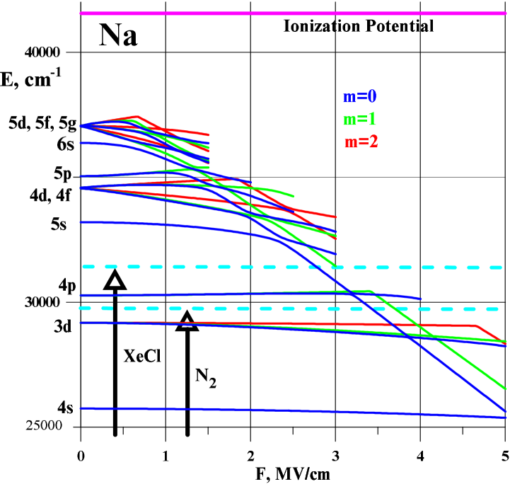
Figure 2: Overview of Stark splitting in Na for m=0,1,2.

The diagram of the splitting of the levels calculated with STARK-I programme is shown on Fig.2. These calculations were performed for a wide range of levels with n=2,3,4,5 and up to 5 MV/cm electric field strength. The Stark effect of higher-lying levels is calculated up to 1.5 MV/cm, where these lines disappear [8, 9, 10]. The lower level shifts are calculated up to 5 MV/cm. The main feature of the splitting seen in Fig.2 is the common shift of all the levels to lower energy. This figure is a subject of analysis for selection of working levels for experiments.

3 Selection of the levels

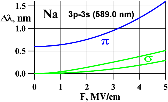
Figure 3: Splitting of 3p-3s transition.

Preliminary consideration of the sodium levels shows us that only a few levels meet all the requirements listed in Sec.2. The first is the 3p level that can be excited from the ground state level 3s by a dye laser with wavelength 589.0–589.6 nm [7]. The 3p–3s transition is a strong one, having an Einstein coefficient $A=6.6\cdot 10^{7}$ s^-1; therefore the lifetime of the 3p level is 15 ns. The second possibility is the 5s level, which can be excited from the 3p level by a dye laser with a wavelength in the range 615.4–616.1 nm. The 5s–3p transition is less strong then the previous one, with an Einstein coefficient $A=0.6\cdot 10^{7}$ s^-1 (the lifetime is 150 ns). The 4d level can also be considered but it can be used for measurements only with an electric field strength below 1.5 MV/cm, because of field ionization.

Since the lifetime of the 3p level is very short, this level must be excited during the accelerator pulse. This is possible with a wide bandwidth laser. Spontaneous fluorescence from the 3p level then gives the shift of spectral line. The long lifetime of the 5s level allows excitation before the voltage pulse, avoiding the need for wide laser bandwidth.

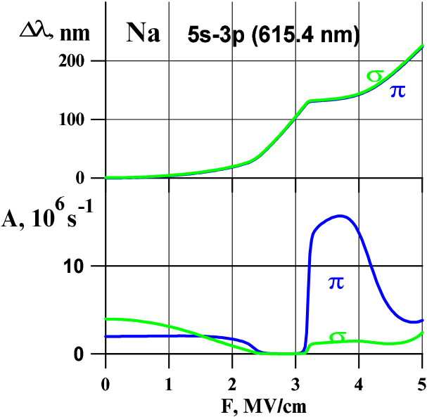
Figure 4: Splitting of 5s-3p transition.

The splitting of a fluorescence spectrum of the 3p–3s transition is illustrated in Fig.3. The splitting is calculated in terms of wavelength shift from the initial wavelength 589.0 nm. The initial splitting is caused by fine structure interaction. Above 2 MV/cm value of electric field strength the splitting becomes big enough for measurement with common spectroscopy apparatus. The intensities of lines are defined both by the population of the upper level and by dipole matrix element between upper and lower states. If a high intensity laser is used the population of the upper level becomes saturated and does not depend on the electric field. The value of population is $({g_{2}}/({g_{1}+g_{2}}))N=(3/4)N$ ($N$ is atomic density). The dipole marix element (or the Einstein coefficient) is almost not depend on electric field strength for this transition. It’s value for $\pi$-component is $2.2\cdot 10^{7}$ s^-1, for $\sigma$-component is $4.4\cdot 10^{7}$ s^-1. These calculated values are in a good agreement with the Einstein coefficient from [7] as all the Einstein coefficients mentioned below.

The level 5s has only one sublevel and the electric field shifts it. However, this level has more possibilities for transition then the 3p. In the high electric field all transitions are possible. In Fig.4, the only one strong line acceptable wavelengthe close to the visible range is shown. The intensities of lines are defined as in previous case by the population of the level $({g_{3}}/({g_{1}+g_{2}+g_{3}}))N=N/5$ and the Einstein coefficient $A$. The difference is that during the electric field pulse the population is not supported by the laser and decreases with time due to fluorescence. The Einstein coefficient of the 5s–3p transition changes dramatically with the electric field rise in contradiction to 3p–3s transition case. The intensity in Fig.4 is equal to the Einstein coefficient $A$ when F=0.

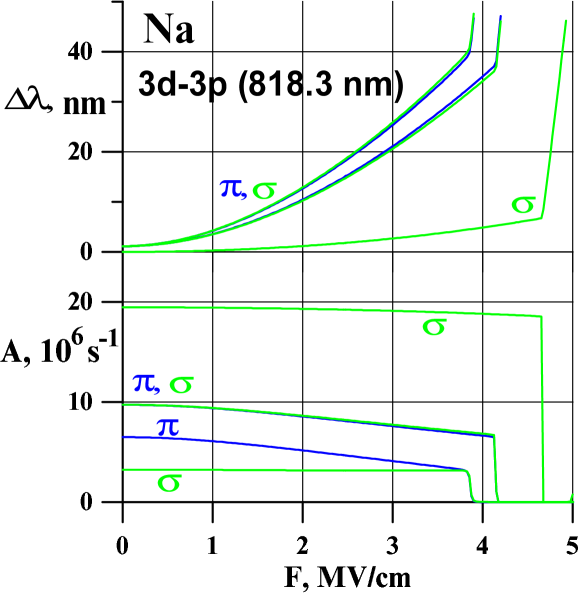
Figure 5: Splitting of 3d-3p transition.

The 3d level can be used with the same way as 5s. The splitting of the 3d–3p transition is shown in Fig.5.

Let us consider next a quite different possibility from the two previous ones for the electric field mearsurement. If we illuminate the sodium atoms with any laser, it could occur that levels can be excited in the presence of the high electric field during the pulse. For example, if we use a XeCl laser (308 nm), the sodium atoms which are located where electric field strength is equal to 2.7 or 3 MV/cm can be excited (see Fig.2). An N₂ laser (337 nm) will excite the atoms where the electric field is 3.4 or 3.7 MV/cm. Any laser should excite the atoms at some value of electric field. If the excited levels have a lifetime longer than the pulse duration the excited levels could provide spontaneous fluorescence and field measurement throughout the pulse. We will call this way of exciting as ”matching” (electric field causes the atom’s excitation energy to match the energy of the laser photon).

Li atoms can be used also in high electric field. However the first transition 2p–2s ($\lambda=670.8$ nm, $A=4\cdot 10^{7}$ s^-1) seems to be difficult because of the small splitting at fields less than 5 MV/cm. The 4s-2p ($\lambda=497.2$ nm, $A=1\cdot 10^{7}$ s^-1), 3d-2p ($\lambda=610.4$ nm, $A=7\cdot 10^{7}$ s^-1), and 3s-2p ($\lambda=812.6$ nm, $A=0.2\cdot 10^{7}$ s^-1) transitions are preferable. The first level has a long lifetime, and it can be used both with excitation just before the pulse and in the ”matching” mode. But in extremely high fields ($>4$ MV/cm) the 4s level will be ionized by the field.

4 Electric field measurement in an ion diode gap

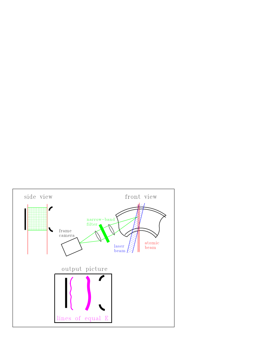
Figure 6: Scheme for observation of equal $|\vec{F}|$ lines.

There are a number of ways of observing the ASAS fluorescence. Figure 6 shows a way to observe lines of equal electric field strength $|\vec{F}|$. A thin rectangular (slab) beam of thermal sodium atoms is introduced into the ion gap. The wide dimension of the slab is parallel to the axis so that the atoms stretch between anode and cathode. The atoms are excited by slab laser beams that have a small pitch angle to the atomic beam in a plane parallel to the anode so that a wide area of atoms will be excited and emit spontaneous fluorescence. An optical system with a narrow band filter gathers the fluorescence and gives an image of the fluorescing area on a frame camera. The filter selects a narrow bandwidth (1$\div$10 nm) of the light which corresponds to a definite electric field strength. The resulting image will show light along lines of equal $|\vec{F}|$.

A similar concept can be realized with ”matching” method. Instead of using a filter the ”matching” method of excitation would used. A short-pulse laser beam irradiates the atomic slab. Atoms are excited only in the regions with definite electric field strengths, where the split components of the spectrum are resonant with the laser wavelegth. The spectral apparatus is not needed. The resulting image shows the lines of constant $|\vec{F}|$. The time gate of the frame camera can be wide because the moment of measurement is defined by the laser pulse. This method appears to be more sensitive than the first.

If the long pulse duration laser will be used for excitation of the levels with a short life time in the ”matching” mode, it is possible to get the movies: a set of pictures with lines of definite $|\vec{F}|$ in different moments of time.

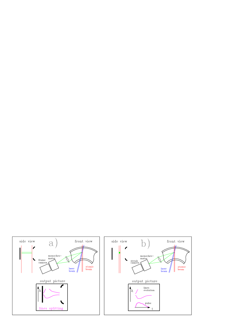
Figure 7: Schemes for electric field measurement.

A method using a monochromator is illustrated by Fig.7a. A thin coloumn of excited atoms is imaged by a lens on the input slit of the monochromator so that the distance along the slit images the distance between anode and cathode. The output of the frame camera gives a two-dimensional picture: the horizontal axis is the distance between anode and cathode, and the vertical axis is wavelength. The electric field variation in the gap can be obtained from this picture. In addition the effect of line disappearance provides a further check on the electric field measurement.

Replacement of the frame camera by a streak camera provides the possibility to see the dependance of a local electric field strength in a time (Fig.7b). The effect of field ionization can also be observed.

5 Summary

The choice of concrete scheme of realization of ASAS technique depends on the device where the diagnostics whould be applied and the goals of the experiment. But it must be pointed out that the most simple way for getting the result is the ”matching” mode of ASAS. It is needed only one laser and unit for registration. The spectral apparatus is not needed!

References

- [1] Y. Maron, M.D. Coleman, D. Hammer, H.-S. Peng. Phys. Rev. Lett., 57, 699 (1986).
- [2] J. Bailey, A. Filuk, A.L. Karlson et.al. Atomic processes in plasmas. 10th Topical Conference, San Francisco, 1996. AIP Conf. Proc. 381 245 (1996).
- [3] B.A. Knyazev, S.V. Lebedev, P.I. Melnikov. Zh. Tekh. Fiz. 61, 6 (1991) [Sov. Phys. Tech. Phys., 36, 250 (1991)].
- [4] B.A. Knyazev, S.V. Lebedev, P.I. Melnikov. Pis’ma Zh. Tekh. Fiz. 17, 16 (1991) [Sov. Tech. Phys. Letters, 17, 357 (1991)].
- [5] H.A.Bethe and E.E.Salpeter. Quantum Mechanics of One- and Two-Electron Atoms. Springer-Verlag, Berlin-Göttingen-Heidelberg, 1957.
- [6] B.A. Knyazev, S.V. Lebedev, P.I. Melnikov. Preprint No.87-60, Institute of Nuclear Physics, Novosibirsk, USSR, 1987.
- [7] W.L.Wiese, M.W.Smith, and B.M.Miles. Atomic Transition Probabilities. Volume II. Sodium Trough Calcium. NSRDS-NBS 22, October 1969.
- [8] Gebauer, R., Traubenberg, H. Z. Phys. 1930, 62, 289-307.
- [9] Traubenberg, H., Gebauer, R., Lewin, G. Naturwissenshaften 1930, 417-421.
- [10] Lanczos C. Z. Phys. 1931, 68, 204-209.