The Hopgrid algorithm: multilevel synthesis of multigrid and wavelet theory

Abstract

The multigrid algorithm is a multilevel approach to accelerate the numerical solution of discretized differential equations in physical problems involving long-range interactions. Multiresolution analysis of wavelet theory provides an efficient representation of functions which exhibit localized bursts of short length-scale behavior. Applications such as computing the electrostatic field in and around a molecule should benefit from both approaches. In this work, we demonstrate how a novel interpolating wavelet transform, which in itself is the synthesis of finite element analysis and wavelet theory, may be used as the mathematical bridge to connect the two approaches. The result is a specialized multigrid algorithm which may be applied to problems expressed in wavelet bases. With this approach, interpolation and restriction operators and grids for the multigrid algorithm are predetermined by an interpolating multiresolution analysis. We will present the new method and contrast its efficiency with standard wavelet and multigrid approaches.

1 Introduction

Many applications such as electronic structure calculations require an efficient method to solve discretized linear differential equations which are generators of long range interactions, such as Poisson’s equation. In modern electronic structure calculations, except those using planewaves, solving Poisson’s equation takes up a significant amount of computational time. It is essential to produce an algorithm that has the capacity to solve efficiently problems involving such long range interactions.

The multigrid algorithm is the state of the art in solving discretized linear differential equations describing long range interactions. It uses a basic iterative method, such as the weighted Jacobi method, over a sequence of scales to iterate faster toward the exact solution. In some cases, even multigrid does not produce sufficiently rapid convergence, particularly in calculations using wavelet bases.

Multiresolution analysis, from wavelet theory, provides the ability to carry out calculations on non-uniform grids, focusing resolution only in regions where it is needed. It is especially useful if the local region which requires high resolution moves through space during the calculation, as when the atoms move in a molecule in an electronic structure calculation. However, a basis set alone does not provide computational efficiency.

Often, a finite element basis set provides the analytic framework for multigrid calculations. Combining the advantages of finite element analysis and the multigrid algorithm with wavelet theory, could provide a very powerful method to solve discretized linear differential equations. This present research aims to unify these approaches for use in a wide range of applications, especially in electronic structure calculations, where all of the aforementioned approaches prove to be very beneficial in various stages of the calculations individually.

A basis set that combines wavelet theory with finite element analysis exists and is known as the interpolet basis (Interpolets is based upon Deslauriers and Dubuc scaling functions [4], which play the role of both scaling functions and interpolets in the interpolet basis. See also [5]). The present research forms a natural bridge in the synthesis of the multigrid algorithm with this basis, thereby adding the power of multiresolution analysis to the multigrid algorithm. In particular, we introduce this new Hopgrid algorithm for use in problems where an underlying wavelet or interpolet basis is necessitated by the problem at hand and application of multigrid algorithm could provide very useful in solving linear differential equations in the problem.

In Section 2 of the paper, to establish a common notation, we give a brief overview of the traditional multigrid algorithm and the iterative methods that form the framework for this algorithm. Section 3 introduces the interpolet theory. Section 4 includes the description of non-orthogonal multiresolution analysis from wavelet theory in the interpolet basis. Section 5 presents the basic ideas behind expressing the multigrid algorithm in the interpolet basis, and describes how such a union becomes more efficient by using multiresolution analysis. Section 6 introduces the new algorithm formed by a more impact synthesis of the multigrid algorithm and the interpolet basis, the Hopgrid Algorithm. The last section expresses the results obtained using this new algorithm. The appendix of this paper aims to familiarize the reader with the essentials of the multigrid algorithm with a thorough discussion of the basic iterative methods and the framework of this algorithm.

2 Multigrid Algorithm

This section briefly summarizes the multigrid algorithm [2] and the interpolation and restriction operators used in this algorithm. A more detailed description of the multigrid algorithm and these operators, aimed for the physicist, may be found in Section 9. Throughout this section, superscripts are used to refer to the scale on which a particular level of the problem is solved.

2.1 Full V-cycle Multigrid Algorithm

The multigrid algorithm is used to solve discretized linear differential equations of the form,

$$Au=f,$$ (1)

where $A$ is the linear operator, $u$ is the solution vector, and $f$ is the source vector. Multigrid is based upon a basic iterative method, which is then applied over a sequence of scales in order to improve the convergence rate. One such iterative method used for this purpose is the weighted Jacobi method, which provides the following recursion,

$$v_{(n+1)}=v_{(n)}+wD^{-1}r_{(n)}.$$ (2)

Here, $w$ is an appropriate weight (usually chosen to be $w=2/3$), $v_{(n)}$ is the initial guess, $D$ is the diagonal matrix composed of the diagonal elements of $A$, and $r_{(n)}$ is the residual at step $n$, defined as $r_{(n)}=f-Av_{(n)}$. We refer to application of this recursion as relaxation.

Multigrid exploits this basic iterative method in a multiscale fashion through the following procedure. First, $\alpha$ relaxations are performed on the scale on which the problem is defined. Then, the residual $r^{(0)}$ is transfered up to a spatially coarser scale, using a linear restriction operator, $r^{(1)}=R_{(0)}^{(1)}r^{(0)}$. On this coarser scale, one then solves the error equation $A^{(1)}e^{(1)}=r^{(1)}$, relaxing again $\alpha$ times. (Note that, as discussed in the appendix, the exact solution to the error equation, when summed with the current iterative solution $v$, yields the exact solution to the problem $u$.) The procedure of passing up the residual to successively coarser scales continues until a predetermined coarsest scale $n$ is reached. At this coarsest scale $n$, one then transfers the solution vector $v^{(n)}$ down to the next finer scale $n-1$ using a linear interpolation operator $I_{(n)}^{(n-1)}$. The error equation is then relaxed on this scale $\beta$ times, using $v^{(n-1)}+I_{(n)}^{(n-1)}v^{(n)}$ as the initial guess. This procedure is followed down to the finest scale, relaxing $\beta$ times at each scale $i$ with the initial guess $v^{(i)}+I_{(i+1)}^{(i)}v^{(i+1)}$, where finally one relaxes $\beta$ times on the original linear equation to obtain an approximate solution to the overall problem.

The procedure described above is the V-cycle of the multigrid algorithm. V-cycles may be repeated in succession to produce a solution of any desired accuracy.

2.2 Theory for Interpolation and Restriction Operators

The interpolation and restriction operators should obey two conditions, known as the variational properties. The first condition, the Galerkin condition, requires that

$$A^{(n+1)}=R_{(n)}^{(n+1)}A^{(n)}I_{(n+1)}^{(n)}.$$ (3)

It is a recipe for the linear operator to be used in relaxations on the next coarser scale. The second condition states that

$$R_{(n)}^{(n+1)}=c(I_{(n+1)}^{(n)})^{T},$$ (4)

where $c$ is a scalar constant. This is the recipe for the restriction operator, up to an overall scalar constant, given the interpolation operator.

3 Interpolet Theory

In this section, we briefly review interpolet theory based on the discussion in Lippert, Arias and Edelman [1].

In interpolet theory, functions varying slowly over integer length scales can be closely approximated as linear combinations of interpolating functions,

$$f(x)=\sum_{n}f_{n}{\cal I}(x-n),$$ (5)

where the $f_{n}$ are the expansion coefficients and the ${\cal I}(x-n)$ are functions with compact support, also known as interpolets.

Interpolets are a basis set combining wavelet theory with finite element analysis. In place of the orthonormality condition common in wavelet theory, interpolets have cardinality and interpolation from finite element analysis as their characteristic properties. We will first discuss the properties which interpolets share with finite elements and then we will describe those properties which they share with traditional wavelets.

Cardinality means that the values of a function are zero at all integers except for zero,

$${\cal I}(n)=\delta_{n0},\,\,\,\mbox{for all integers $n$}.$$ (6)

As a consequence of this condition, the function formed by the linear expansion in Eq. (5) will match exactly the value of the original continuous function at the integer grid points when the expansion coefficients are taken to be the values of $f(x)$ at the integers, $f_{n}\equiv f(n)$,

$$f(n)=\sum_{m}f_{m}{\cal I}(n-m)=\sum_{m}f_{m}\delta_{nm}=f_{n}.$$ (7)

Interpolation is the further condition that Eq. (5) reproduces any polynomial, up to order L for all $x$,

$$x^{k}=\sum_{n}n^{k}{\cal I}_{L}(x-k),\,\,\,k=0,1,...,L,$$ (8)

where subscript $L$ denotes the order of interpolation. Given the values of a function at the integers, interpolets then provide a compact estimate correct to $L^{th}$ order of the values of the function at the half integers through

$$f(\frac{x}{2})=\sum_{m}f_{m}{\cal I}_{L}(\frac{x}{2}-m).$$ (9)

The matrix representations for the interpolation operators defined by this relation for both first order interpolets ($L=1$) and third order interpolets ($L=3$) are given below. Note that the $L=1$ case gives the familiar linear interpolation procedure. and that the $L=3$ case is distinct from the interpolation given by traditional cubic $B-$splines. Interpolet theory thereby provides guidance in selecting natural interpolation operators for use in the multigrid algorithm.

$${\cal I}_{L=1}=\left(\begin{array}[]{c c c c c c}\ddots&&&&&\\ &\frac{1}{2}&&&&\\ &1&&&&\\ &\frac{1}{2}&\frac{1}{2}&&&\\ &&1&&&\\ &&\frac{1}{2}&\frac{1}{2}&&\\ &&&1&&\\ &&&\frac{1}{2}&\frac{1}{2}&\\ &&&&1&\\ &&&&\frac{1}{2}&\\ &&&&&\ddots\\ \end{array}\right),$$

$${\cal I}_{L=3}=\left(\begin{array}[]{c c c c c c}\ddots&&&&&\\ &-\frac{1}{16}&&&&\\ &0&&&&\\ &\frac{9}{16}&-\frac{1}{16}&&&\\ &1&0&&&\\ &\frac{9}{16}&\frac{9}{16}&-\frac{1}{16}&&\\ &0&1&0&&\\ &-\frac{1}{16}&\frac{9}{16}&\frac{9}{16}&-\frac{1}{16}&\\ &&0&1&0&\\ &&-\frac{1}{16}&\frac{9}{16}&\frac{9}{16}&\\ &&&0&1&\\ &&&-\frac{1}{16}&\frac{9}{16}&\\ &&&&0&\\ &&&&-\frac{1}{16}&\\ &&&&&\\ &&&&&\ddots\\ \end{array}\right)$$

In addition to properties from finite element analysis, interpolets satisfy the central condition of wavelet theory, the two-scale relation. This relation states that every coarse scale interpolet is expressible as a linear combination of finer scale interpolets. Interpolets therefore interpolate themselves exactly,

$${\cal I}_{L}(x)=\sum_{n}c_{n}{\cal I}_{L}(2x-n).$$ (10)

Here, the ${\cal I}_{L}(x)$ is the coarse scale interpolet, the ${\cal I}_{L}(2x-n)$ are fine scale interpolets, and the $c_{n}$ are the expansion coefficients. (Note that from the cardinality property, we have that the $c_{n}$ are just the values of the interpolet at the half-integers $c_{n}={\cal I}_{L}(n/2)$.) The significance of this condition is to ensure that a basis made from interpolets of varying scales always provides a very uniform description of space. This point is described in detail the next section.

x	-2	-$\frac{3}{2}$	-1	-$\frac{1}{2}$	0	$\frac{1}{2}$	1	$\frac{3}{2}$	2
l=1			0	$\frac{1}{2}$	1	$\frac{1}{2}$	0
l=3	0	-$\frac{1}{16}$	0	$\frac{9}{16}$	1	$\frac{9}{16}$	0	-$\frac{1}{16}$	0

Table I: Values of interpolets of orders $l=1,3$ at various points $x$ within their compact support. Values not shown are zero.

The self-interpolation property may be applied recursively to express an interpolet in terms of interpolets on arbitrary finer scales,

$${\cal I}_{L}(x) = \sum_{n}\sum_{m}\,...\,\sum_{k}c_{n}c_{m}\,...\,c_{k}$$

$$\times\ \ {\cal I}_{L}(2^{a}x-2^{a-1}n-2^{a-2}m\,...\,-k)$$

$$= \sum_{k}{\cal I}_{L}(k/2^{a}){\cal I}_{L}(2^{a}x-k).$$

where $a$ is a positive integer that determines the fine scale on which the original interpolet is expanded. This relation gives a procedure for determining the values of any interpolet recursively once given the values of the $c_{n}$. Table I presents these expansion coefficients from which the interpolets may be constructed through the two-scale relation.

4 Non-orthogonal Multiresolution Analysis

Figure 1: This figure illustrates pictorially how an MRA basis is created. The bigger circles represent the coarse scale interpolets, while the smaller circles are for the fine scale interpolets.

In this section, we present a brief discussion of multiresolution analysis (MRA) of interpolet and wavelet theories [1],[3], and the application of MRA to non-uniform grids such as the ones employed in electronic structure problems.

Assume that there is a basis spanning a space $V_{0}$ as in Figure 1a. We refer to this space $V_{0}$ as the coarse real space and this representation as the direct representation. In this space, any function $f(x)$, varying slowly over the given grid spacing, can be approximated with a linear combination of interpolets of the appropriate scale as explained in the previous section,

$$f(x)=\sum_{n}f_{n}{\cal I}_{L}(x-n).$$ (12)

To double the resolution of this basis, we can double the number of grid points and decrease the scale of the basis functions by a factor of two, as Figure 1b illustrates. In this new space, $V_{1}$, which we refer to as the fine real space, any function $f(x)$ varying slowly over the new grid spacing can be approximated with a linear combination of fine scale interpolets with half the compact support as

$$f(x)=\sum_{n}\tilde{f}_{n}{\cal I}_{L}(2x-n).$$ (13)

General wavelet theory provides another tool to enhance the spatial resolution of the basis in Figure 1a, locally. This tool is known as multiresolution analysis (MRA). MRA states that to double the resolution of a given basis, we may add to the existing basis a new set of functions spanning a space $W_{0}$, such that $V_{0}+W_{0}=V_{1}$. For this condition to hold, we need to prove the two constraints that these spaces should satisfy, namely $V_{0}+W_{0}\supset V_{1}$ and $V_{0}+W_{0}\subset V_{1}$. In order for the first condition to hold, it is sufficient that the interpolets satisfy the two-scale relation, Eq. (10) of Section 3. In order to prove the second condition, one must show that any interpolet ${\cal I}_{L}(2x-n)\in V_{1}$ can be written as a linear combination of interpolets in the space $V_{0}+W_{0}$. (This is proven for interpolets in [1].) The new basis spanning the space $V_{0}+W_{0}$ is illustrated in Figure 1c. Henceforth, we will refer to such a mixed basis space as the MRA space and such a representation as the MRA representation.

The MRA basis can be extended to include not only the next finer scale but other scales of increasing fineness, as Figure 1d illustrates. Adding $W_{i}$’s ($i=0,1,2,...,N$) to $V_{0}$ improves the resolution of the original space by a factor of $2^{N+1}$,

$$V_{N}=V_{0}+W_{0}+W_{1}+...+W_{i}+...+W_{N-1}.$$

Multiresolution analysis is especially useful when the problem requires only local regions of high resolution and only a small fraction of the expansion coefficients for the MRA basis are significant. Under these circumstances, one needs to employ only a small subset of the full MRA basis. We shall refer to the points in space associated with the remaining basis functions as the non-uniform grid for the problem. In electronic structure problems, for instance, only a small spherical region around the atomic core requires high resolution to describe the most rapid oscillations in the electronic wave functions. Such problems are best addressed using non-uniform grids where high densities of grid points are concentrated in concentric spheres with differing resolution surrounding the atomic nuclei. The advantage of using such an MRA basis appears when the nuclei move. New grids do not have to be generated, and associated Pulley forces calculated, as the nuclei move. Rather, high resolution MRA basis functions may be simply turned on and then off as nuclei pass by. [1] provides a more detailed explanation of this application.

5 Combining the Multigrid Algorithm with Interpolets and MRA

We have so far described the multigrid algorithm and the interpolet basis. In this section, we discuss the rationale for combining the multigrid algorithm with interpolets. The result of Section 5.1 will be an algorithm in the direct representation. We will discuss multiresolution algorithms in Section 5.2.

5.1 Choice of Interpolation and Restriction Operators

Interpolets provide a natural prescription for an interpolation operator to be used in the multigrid algorithm. However, multigrid also requires an appropriate restriction operator so that both variational properties are satisfied. In this section we will see that the appropriate restriction operator is just the transpose of the interpolet interpolation operator. This comes about because of the form of linear operators generated by applying the Galerkin technique to the interpolet basis.

Let the following be the $d$-dimensional linear equation to be solved,

$$\hat{\cal O}\phi(x)=\rho(x),$$ (14)

where $\hat{\cal O}$ is a linear operator and $\phi(x)$ and $\rho(x)$ are functions of the $d$-dimensional variable $x$. If we are to solve this equation in an interpolet basis, $\phi(x)$ and $\rho(x)$ are then expanded as,

$$\phi(x)=\sum_{n}\tilde{\phi}_{n}{\cal I}_{L}(x-n),\,\,\rho(x)=\sum_{n}\tilde{\rho}_{n}{\cal I}_{L}(x-n).$$ (15)

Substituting these expansions into the linear equation and applying $\int dx\,\,{\cal I}_{L}(x-m)$ to both sides yields

$$\sum_{n}A^{(n)}_{mn}\tilde{\phi}_{n}=\sum_{n}U^{(n)}_{mn}\tilde{\rho}_{n},$$ (16)

where

$$A^{(n)}_{mn}\equiv\int dx\,\,{\cal I}_{L}(x-m)\,\,\hat{\cal O}{\cal I}_{L}(x-n)$$ (17)

is the interpolet form for the linear operator on scale $n$, and

$$U^{(n)}_{mn}\equiv\int dx\,\,{\cal I}_{L}(x-m){\cal I}_{L}(x-n).$$ (18)

Using the two scale relation, we may relate this operator to the linear operator on the next coarser scale $A^{(n+1)}$,

$$A^{(n+1)}_{mn} \equiv \int dx\,\,{\cal I}_{L}(x/2-m)\hat{\cal O}{\cal I}_{L}(x/2-n)$$

$$= \sum_{kl}c_{k}c_{l}\int dx\,\,{\cal I}_{L}(x-2m-k)\,\,\hat{\cal O}{\cal I}_{L}(x-2n-l)$$

$$= \sum_{kl}c_{k}A_{2m+k,2n+l}^{(n)}c_{l}$$

$$A^{(n+1)} = {\cal I}_{L}^{T}A^{(n)}{\cal I}_{L}.$$ (19)

In the final line, we convert the relationship between the operators on the two scales into a matrix equation. From Eq. (19), we may construct a set of operators that automatically satisfy both variational properties, the Galerkin condition and the full weighting condition. The appropriate set of operators are as follows. First, the linear operators $A^{(n)}$ representing $\hat{\cal O}$ will be those generated from the interpolets using the standard Galerkin procedure. Second, the interpolation operators ${\cal I}_{L}$ will be those generated from the interpolets as discussed in Section 3. Finally, this analysis shows that to complete the set, the restriction operators must be $R={\cal I}_{L}^{T}$.

Implementing the interpolet basis in the multigrid algorithm is then using the linear operators $A^{(n)}$ to solve Eq. (1) and the error equation, and using the matrices ${\cal I}_{L}$ and ${\cal I}_{L}^{T}$ as the interpolation and the restriction operators, respectively.

5.2 Synthesis of MRA into the Interpolet Multigrid Algorithm

In this section, we discuss how we may generalize the algorithm that combines the interpolet basis with the multigrid algorithm to multiresolution bases. We also discuss briefly how this multigrid algorithm in the MRA bases may be applied to non-uniform grids in an efficient manner.

Figure 2: Interpolation and restriction operations carried out in the MRA representation. The arrows indicate the direction to follow to carry out interpolation and restriction. The larger (smaller) circles represent the coarser (finer) scale interpolets.

We will now discuss two approaches for carrying out interpolation and restriction for data in the MRA representation illustrated in Figure 2a. The first approach is a direct approach and is equivalent to the method explained in the previous section. To carry out restriction in this approach, one first changes from the MRA representation to the direct representation (the process carrying data from Figure 2a to Figure 2b. One then carries out the restriction operation in the usual way by applying the previously described linear operator ${\cal I}_{L}^{T}$ (making the transformation Figure 2b$\rightarrow$2c). Finally, one converts back from the direct representation to the MRA representation (2c$\rightarrow$2d). Interpolation within this approach also consists of three steps. First, we change from the MRA representation to the direct representation (2d$\rightarrow$2c), then we carry out interpolation with the usual operator ${\cal I}_{L}$ (2c$\rightarrow$2b), and finally we convert back from the direct representation to the MRA representation (2b$\rightarrow$2a). We refer to this approach of changing from the MRA representation to the direct representation in order to carry out the interpolation and the restriction operations as the operator method.

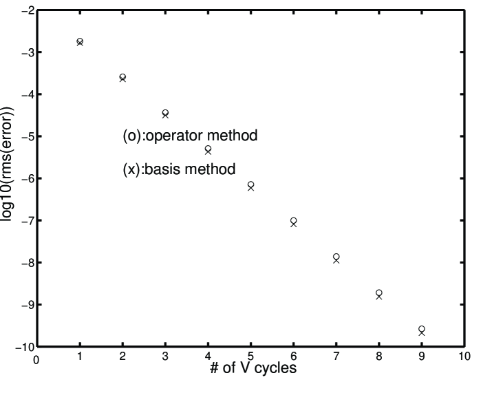
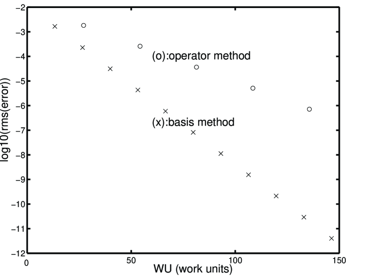
Figure 3: The operator method compared to the basis method. The first figure represents the convergence rate vs the number of V-cycles and the second figure shows that the convergence rate of the basis method is computationally more efficient when the number of work units are considered. The above graphs are obtained by solving the Poisson’s equation on a grid of 128 points, using first order interpolets.

The second approach is an improvement upon the operator method. This approach uses the properties of the MRA basis to carry out the operations of interpolation and restriction entirely within the MRA representation. We refer to this second method as the basis method. It uses the general physical meaning of restriction and interpolation to exploit the interpolet basis. Restriction is the elimination of the fine information from a given basis and mapping it onto a coarser one. In the interpolet basis, this fine information corresponding to the high frequency modes is carried by the finest interpolets. Therefore, restriction in this basis corresponds to the obviation of all the coefficients for the finest interpolets. Interpolation maps coarse information onto a finer grid. In the interpolet basis, the coarse information is represented by the coarse interpolets. Thus, interpolation leaves the coarse interpolets unaffected, padding the coefficients for all finer interpolets with zeros.

The operators in this new method satisfy the Galerkin condition since the interpolation operator in the MRA representation consists of a block identity matrix and a block zero matrix for the coarse and fine informations respectively. Figure 3a illustrates that the operator and the basis methods are equivalent with the same convergence rates per V-cycle.

Note that the basis basis method has three distinct advantages over the operator method. First, the basis method requires no matrix-vector multiplications to implement interpolation and restriction. Figure 3b illustrates that the basis method is superior to the operator method on a per flop basis. Second, the basis method provides the abilities to interpolate and to restrict over many scales in a single step. Finally, the basis method is easily generalized to problems on non-uniform grids. On non-uniform grids, restriction is merely obviation of finer scale coefficients and interpolation is padding finer scale coefficients with zeros.

6 The Hopgrid Algorithm

In this section we introduce the Hopgrid algorithm, which is the synthesis of the multigrid algorithm and the interpolet basis in the MRA representation. We present Hopgrid as an algorithm to solve discretized linear differential equations on interpolet bases in MRA representation.

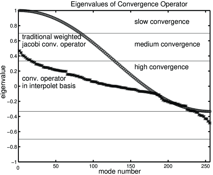
Figure 4: Eigenvalue spectrum of the convergence operators for the weighted Jacobi method in the traditional multigrid basis and the interpolet MRA basis for a problem of 256 grid points. For the eigenvalue spectrum of the traditional weighted Jacobi operator, w=2/3, and for the weighted Jacobi operator in the interpolet MRA basis, w=1.

The efficiency of using the interpolet MRA basis in the multigrid algorithm appears when we look at how the error behaves at each step. The error vector at iteration step $n$ is

$$e_{(n)}=A^{-1}f-v_{(n)}.$$ (20)

Substituting the definition of the residual, $r=f-Av$ and Eq. (2) into Eq. (20) returns the following expression, which states that error at each step is multiplied by a convergence operator

$$e_{(n+1)}=\hat{\cal C}e_{(n)}$$ (21)

where $\hat{\cal C}\equiv 1-wD^{-1}A$. The eigenvalues of this operator determine how the error behaves at each iterative step. Figure 4 illustrates the eigenvalue spectrum of the convergence operators for both the traditional weighted Jacobi method and the weighted Jacobi method in the interpolet MRA basis.

The convergence bands shown in Figure 4 are chosen for convenience to describe the effects of the eigenvalues on the error modes. The high convergence band is defined to be the region in which the choice of $w$ for the weighted Jacobi recursion guarantees that about half of the eigenvalues of the convergence operator of the traditional weighted Jacobi method lie in the vicinity of zero. The errors which are multiplied by these eigenvalues approach zero at a high rate. The medium convergence band and the slow convergence band are the regions where the convergence of the error to zero is slower. The distinction between these two bands in Figure 4 is chosen for purposes of illustration.

First, we will consider the convergence of the traditional weighted Jacobi method. The choice of weight $w$ in the method affects the number of eigenvalues that lie in each of the bands; however, the operator $D^{-1}A$ always has eigenvalues approaching zero, and so the convergence operator always includes eigenvalues near unity and modes which converge very slowly.

On the other hand, most of the eigenvalues of the convergence operator in the interpolet MRA basis are clustered in the high convergence band. The reason for this behavior of the eigenvalues is the fact that the flow of information on the interpolet MRA basis is stronger than the flow of information in the basis which the traditional multigrid algorithm uses. The superiority in communication in the MRA basis comes from the fact that the MRA basis includes functions with support spanning the entire spatial extent of the problem.

The information given in Figure 4 shows that after one weighted Jacobi relaxation in the interpolet MRA basis, most of the error modes are eliminated. Only the modes that correspond to the eigenvalues at the edges of the spectrum survive after relaxation. Numerical experiments show that these surviving error modes have low spatial frequencies and so may be eliminated very efficiently, using the basic ideas underlying the traditional multigrid algorithm.

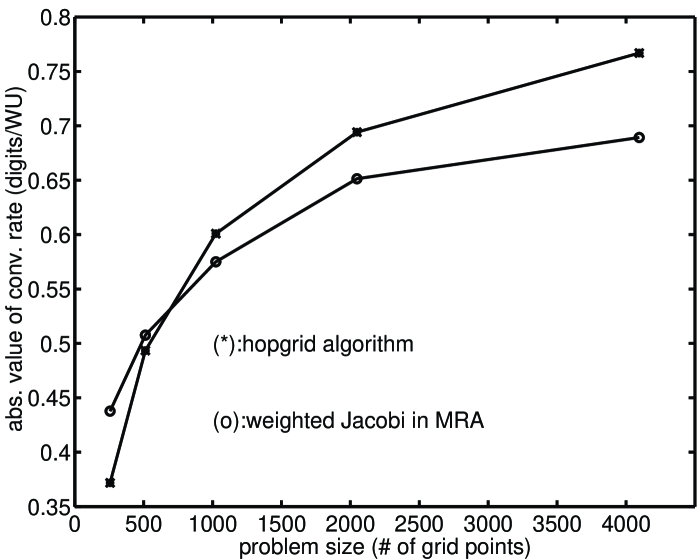
Figure 5: Comparison between the weighted Jacobi method in the MRA representation and the Hopgrid algorithm for the solution of Poisson’s equation on grids of several different sizes.

We now exploit these observations to produce a new algorithm. The basic outline of the algorithm is to first use weighted Jacobi in the MRA representation to eliminate the error modes that correspond to the high frequency eigenvalues in the high convergence band, and then to restrict the residual to a very coarse spatial scale where the error equation is solved exactly, eliminating the remaining error modes. The fact that we hop over many scales in order to produce the error vector gives this new algorithm its name, the Hopgrid Algorithm. Below we shall refer to the scale on which we solve the error equation as the hop scale, $h$. Figure 5 shows the comparison between the convergence rates in digits/WU (work unit) vs problem size for the Hopgrid algorithm and the weighted Jacobi method in the MRA representation. As this figure illustrates, the hopping over many scales to calculate the error improves the convergence rate, especially with increasing problem size.

The detailed procedure for the Hopgrid algorithm is as follows. First, one applies weighted Jacobi in MRA representation once on the finest scale ($\alpha$=1) to find an approximate solution vector $v^{(0)}$. Then, to reduce the computational overhead of the algorithm, instead of calculating all the entries of the residual $r^{(0)}=f-Av^{(0)}$, we calculate only the $2^{h}$ entries which correspond to the restricted residual on the hop scale $h$. Furthermore, because these entries depend only weakly on the high frequency components of $v^{(0)}$, we compute them only with the $2^{h+2}$ entries of $v^{(0)}$ corresponding to the hop scale with two levels of refinement. After hopping over many scales, the number of grid points on $h$ is very small compared to the number of points on the finest scale, so that, now, solving the error equation, $A^{(h)}e^{(h)}=r^{(h)}$ exactly becomes a negligible part of the computation. Finally, we hop again over many scales and interpolate the resulting $e^{(h)}$ back to the finest scale, again just padding with zeros. The sum of the approximate solution before hopping $v^{(0)}$ and the interpolated error from scale $n$ gives the improved solution vector $v=v^{(0)}+I_{(n)}^{(0)}e^{(n)}$. The hopping procedure may then be applied recursively to reach any desired level of accuracy.

Numerical experiments show that the best convergence rates are obtained when the hop scale $h$ is chosen so that $h\leq\frac{N}{2}$, where $N$ is defined such that the number of grid points for the original problem is $2^{N}$.

7 Results

In this section we compare the efficiency of the Hopgrid algorithm with the traditional multigrid algorithm. We use two different measures of convergence rate for comparison. The first measure is the conventional measure in terms of digits per WU [2]. Here, we define one work unit to be the number of flops it takes to multiply a vector by the matrix representing the linear operator in the corresponding basis. We will see that in terms of this measure the present algorithm is signficantly superior. The MRA representation loses part of its advantage in problems requiring uniform resolution, as on a uniform grid, MRA operators are far denser, having fractal dimension 1.5, than their single scale counterparts. Even in this extreme case, the Hopgrid algorithm overcomes the appearant disadvantage of the density of the MRA operators. To demonstrate this we also compare the convergence rates of the two algorithms on a per flop basis. Note that we envision applying the Hopgrid algorithm to non-uniform problems expresses in MRA representations and the flop count for the uniform case represents a worse-case scenario.

Figure 6: Source vector and the exact solution to Poisson’s equation that is used in finding the results shown in this section.

The results presented in this section all use third order interpolets. The differernatial equation we solve for our tests is the Poisson Equation in one dimension on the unit interval with periodic boundary conditions,

$$-\frac{\partial^{2}}{\partial x^{2}}\phi(x)=\rho(x).$$ (22)

As Figure 6 illustrates, we use for testing purposes two $\delta$-functions of weight one with opposite signs as the source vector $\rho(x)$. Given this source vector, the exact (both analytic and numeric) solution to Poisson’s equation, $\phi(x)$, is the piece-wise linear function as given in Figure 6.

Following the procedure given in Section 5.1, we substitute the interpolet basis expansions for $\phi(x)$ and $\rho(x)$ into Eq. (22). In the direct representation, this procedure returns the matrix equation

$$\sum_{n}A_{mn}\tilde{\phi}_{n}=\sum_{n}U_{mn}\tilde{\rho}_{n},$$ (23)

where $A_{mn}=\int dx\,\,\frac{d}{dx}{\cal I}_{L}(x-m)\frac{d}{dx}{\cal I}_{L}(x-n)$ and $U_{mn}=\int dx\,\,{\cal I}_{L}(x-m){\cal I}_{L}(x-n)$. These are the matrix elements employed in the traditional multigrid calculations, numerical values computed by recursive application of the two scale relation as described in [1], are provided in Table II.

For $A_{mn}$, values for $\mid m-n\mid$ :	0	1	2	3	4	5
First order interpolet:	-2	1	0
Third order interpolet:	$\frac{20}{9}$	-$\frac{9}{8}$	0	$\frac{1}{72}$	0	0

Table II: Non-zero matrix elements for the linear operator $A_{mn}$ for the first and the third order interpolets. The matrix elements for the fifth order interpolets can be calculated in a straight forward manner but are not listed here.

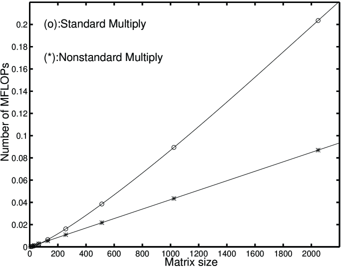
Figure 7: The standard matrix vector multiplication by the linear operator in the MRA basis vs the non-standard multiplication.

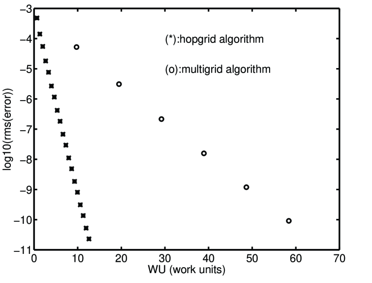
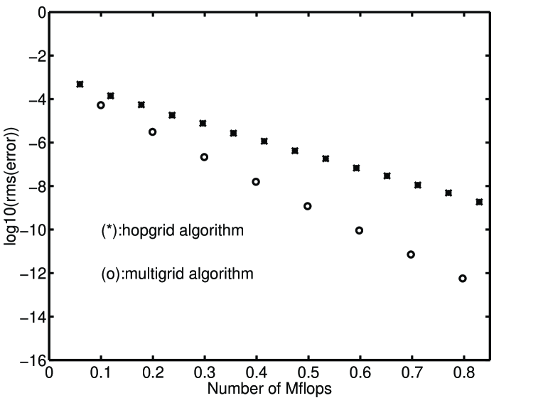
Figure 8: The convergence of the traditional multigrid algorithm versus the convergence of the Hopgrid algorithm for the solution of the Poisson’s equation on a grid of 1024 points.

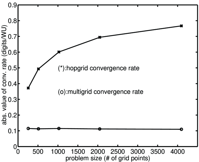
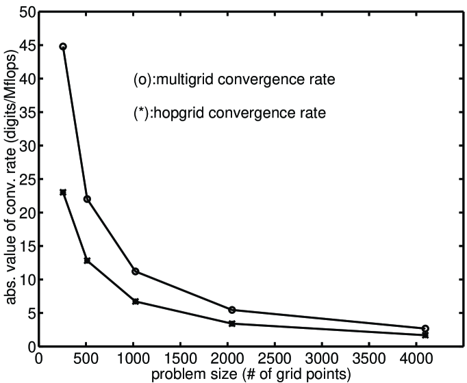
Figure 9: Comparison between the convergence rates of the traditional multigrid algorithm and the Hopgrid algorithm for increasing problem size.

The Hopgrid calculations require matrix elements of the linear operator in the MRA represenation. These elements are

$$A_{mn}^{mra}=\int dx\,\,\frac{d}{dx}{\cal I}_{L}(2^{s_{m}}x-m)\frac{d}{dx}{\cal I}_{L}(2^{s_{n}}x-n),$$ (24)

where $s_{i}$ is the scale of basis function $i$. These values may be computed from the previous $A_{mn}$ by appropriate change of integration variable and application of the two scale relation.

Multiplying a vector by this MRA matrix may be performed using one of two different methods. The first is straight forward multiplication by the matrix $A^{mra}$. Because of the density of the MRA matrix mentioned above, the number of flops required to apply the operator within the method grows faster than linearly with the size of the problem. The second approach uses the two-scale relation to reduce the number of operations so that the effort in the matrix multiplication scales only linearly with the size of the problem [1]. Figure 7 compares the number of $Mflops$ needed by the standard and the non-standard multiplications as a function of problem size. We use this superior approach in all of our comparisons.

Figure 8 shows how the convergence of the Hopgrid algorithm to the exact solution compares with the convergence of the traditional multigrid algorithm for a problem of 1024 grid points. In Figure 8a, the convergence to the exact solution is plotted against work units (WU). Using this comparison the Hopgrid proceesure is superior to the traditional multigrid algorithm. When the convergence rates of these two algorithms are compared in terms of $digits$ per Mflops, as in Figure 8b, we find that despite the increased density of the MRA matrix (by about a factor of ten), the two methods give comparable results on a uniform grid.

Next we investigate the dependence of these convergence rates on problem size. In terms of $digits$ per $WU$, Figure 9a shows that although the convergence rate of the traditional multigrid algorithm remains nearly constant, the convergence rate of the Hopgrid algorithm increases with increasing problem size. Figure 9b shows that even for the uniform case, the efficiency of the Hopgrid algorithm overcomes the increased complexity of the MRA matrix and results in nearly the same convergence rate as the traditional method in terms of a direct floating point operations comparison. It is in the case of non-uniform grids, where the application of the MRA matrix requires far fewer operations, where we expect the maximum from the new algorithm,

8 Conclusion

In this research, our aim was to develop a new algorithm that benefits from the best combination of a variety of approaches, in particular the multigrid algorithm, multiresolution analysis from wavelet theory, and finite element analysis. The application for the new algorithm which we have in mind is the numerical solution of problems involving long-range interactions where an underlying interpolet basis with its multiresolution properties is needed. We have shown that the interpolet theory, based upon multiresolution analysis from wavelet theory and interpolation properties from finite element theory, provides a natural and unique choice of interpolation and restriction operators and an underlying grid for the multigrid algorithm. Then we showed how the operations of restriction and interpolation may be carried out efficiently, without the application of linear operators, by exploiting the properties of an MRA basis. Finally, we introduced the Hopgrid algorithm, which draws upon these results to produce a multigrid-like method to solve discretized linear equations in problems expressed in multiresolution wavelet bases. We have seen that the convergence rate of the new algorithm in terms of work units is superior to that of the traditional multigrid apprach and that, even in the worse-case scenario of a uniform problem, the new algorithm performs as well as the traditional approach on a direct floating point operation basis despite the increase complexity of MRA matrices.

9 Appendix: Description of the Multigrid Algorithm

In this section, we give a detailed discussion of the traditional multigrid algorithm. This introduction to multigrid is a review of the technique as given in A Multigrid Tutorial by William Briggs [2].

9.1 Basic Iterative Methods And the Coarse Grid Correction Scheme

We first present the weighted Jacobi basic iterative method and the coarse grid correction scheme which are the core ideas in the multigrid algorithm.

Assume that the discretized differential equation we wish to solve may be represented in matrix form as

$$Au=f,$$ (25)

where $A$ is the linear operator, $u$ is the solution vector, and $f$ is the source vector. Given an approximation to the solution, which we will refer to as $v$, the error can be expressed as $e=u-v$. Another measure of error is the residual $r$,

$$r\equiv f-Av.$$ (26)

With this definition,

$$Ae=r$$ (27)

is equivalent to Eq. (25). Henceforth, we shall refer to Eq. (27) as the error equation.

Decomposing the initial matrix $A$ as $A=D-L-U$, where $D$, $-L$, $-U$ are the diagonal, lower triangular and upper triangular elements of $A$ respectively, Eq. (25) becomes

$$u=D^{-1}(L+U)u+D^{-1}f.$$ (28)

This equation may be solved iteratively with the following recursion,

$$v_{(n+1)}=D^{-1}(L+U)v_{(n)}+D^{-1}f.$$ (29)

This recursive algorithm can be improved by choosing an appropriate weight $w$, and taking a weighted average of the initial guess, $v_{(n)}$, and the solution from Eq. (29),

$$v_{(n+1)}=[(1-w)I+wD^{-1}(L+U)]v_{(n)}+wD^{-1}f.$$ (30)

Solving Eq. (26) for $f$ and substituting into Eq. (30) gives a simplified form for this recursion, in terms of the residual alone,

$$v_{(n+1)}=v_{(n)}+wD^{-1}r_{(n)},$$ (31)

where $r_{(n)}$ is the residual at step $n$. This simplified recursion is the core of the basic iterative method known as the weighted Jacobi method. The application of this method for solving a problem is referred to as relaxation.

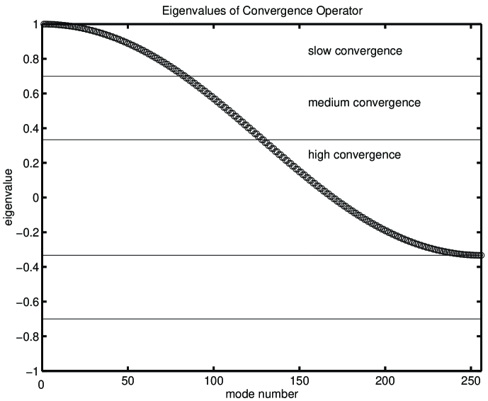
Figure 10: Convergence operator for the weighted Jacobi method.

The weighted Jacobi method and similar basic iterative methods rapidly eliminate high frequency errors while leaving the smooth components of the error mostly unaffected. This is called the smoothing property. The reason for this behavior can be explained when we look at the eigenvalues of the convergence operator $\hat{\cal C}\equiv 1-wD^{-1}A$. The eigenvalues of this operator determine how fast the error converges to zero. Fig. 10 shows that the eigenvalues of the convergence operator for the weighted jacobi method lie in various ranges. The bands are chosen for illustration purposes and an explanation for these choices are given in the main body of the paper.

The errors that are multiplied by the eigenvalues in the slow convergence band correspond to eigenvectors varying slowly in space. Because the convergence operator $\hat{\cal C}$ does not eliminate efficiently most of these low frequency errors, this basic iterative method approach the exact solution very slowly. A more efficient method would eliminate all the error modes at equal rates. The multigrid algorithm has this feature and produces a solution that approaches the analytic solution with a higher convergence rate.

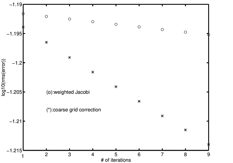
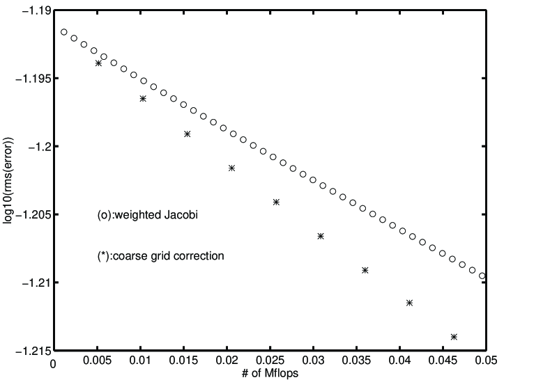
Figure 11: This graph shows the difference between the efficiencies of a pure basic iterative method (weighted jacobi) and the coarse grid correction in finding the solution for the Poisson’s equation on a grid of 128 points.

The transition from the weighted Jacobi method to the multigrid algorithm is made by improving upon the basic Jacobi method. One way to improve the efficiency of weighted Jacobi relaxations is to start with a better initial guess. Conceptually, one can do this by solving the problem on a spatially coarser scale and using this solution as the initial guess for the original problem. This procedure is referred to as coarse grid correction (CGC). On the coarse scale, there are fewer grid points, and on this grid the smooth error modes from the fine scale now appear higher frequency modes. Replacing the original problem with a smaller one of mostly high frequency errors allows the application of the weighted Jacobi method to solve the problem more efficiently. This way, the convergence rate for the total error is accelerated since both the high and the low frequency error modes are eliminated on the fine and the coarse scales.

Figure 11 illustrates the accelerated convergence rate of coarse grid correction scheme compared to the weighted Jacobi method.

9.2 Full V-cycle Multigrid Algorithm

The multigrid algorithm simply extends the idea of CGC over a sequence of scales. Throughout this section, superscripts are used to refer to the scale on which that particular level of the problem is solved.

In order to find an approximation to the solution of the linear equation $Au=f$, we first apply the weighted Jacobi method as in Eq. 31 $\alpha$ times (do $\alpha$ relaxations) on the finest scale, to obtain an approximate solution $v^{(0)}$ and a residual $r^{(0)}$. The residual calculated on this scale is then transferred to the next coarser scale using a linear operator $R_{(0)}^{(1)}$, known as the restriction operator. In general, $R_{(i)}^{(i+1)}$ takes a vector from a fine scale $i$, and transfers it to the next coarse scale $i+1$. (This operator is discussed later in the appendix.) For the restriction step, we assume that the relaxation on the finest scale has eliminated most of the high frequency error components, which lie in the null-space of restriction, so that little information is lost in the restriction process. The restricted residual is now

$$r^{(1)}=R_{(0)}^{(1)}r^{(0)}.$$ (32)

Next we solve the residual equation

$$A^{(1)}e^{(1)}=r^{(1)},$$ (33)

where $A^{(1)}$ is the linear operator on the coarse scale, performing $\alpha$ relaxations, using $e^{(1)}=0$ as an initial guess. This relaxation produces an approximation to the error on the fine scale. We could add this error to $v^{(0)}$ to obtain an approximate solution for the fine scale problem, since $u=v+e$, as previously explained. However, the multigrid algorithm continues to go down to coarser scales and uses CGC to find solutions for the error equations at each coarser scale to improve the convergence rate. Following this prescription, we compute the residual on scale $1$ and transfer it to the next coarser scale, using the restriction procedure described. Repetition of such relaxation and restriction steps continues until the predetermined coarsest scale $n$ is reached. During each step leading up to the coarsest scale, the generated approximate solution vectors, the $v^{(i)}$, and the residuals, the $r^{(i)}$, are stored to be used later in the algorithm. Although the notation used for the result of the relaxations at each scale is $v$, it is important to realize that except for the finest scale on which the original problem is defined, all the vectors $v^{(i)}$ are approximations to the error since the error equation is used during relaxations.

At the coarsest scale, another linear operator, an interpolation operator $I_{(n)}^{(n-1)}$ transfers the approximate solution vector $v^{(n)}$ down to the next finer scale. In general, the interpolation operator $I_{(i+1)}^{(i)}$, takes a vector from a coarse scale $i+1$, and transfers it to the next fine scale $i$. (This operator is also discussed later.) The interpolated approximate solution vector, $I_{(n)}^{(n-1)}v^{(n)}$, is the approximation to the error for scale $n-1$. The sum of the approximate solution $v^{(n-1)}$ and $I_{(n)}^{(n-1)}v^{(n)}$, give the approximate solution on scale $n-1$. However, the interpolation process may introduce high frequency errors into this solution. We eliminate these errors by relaxing $\beta$ times on the residual equation using the initial guess $v_{*}^{(n-1)}=v^{(n-1)}+I_{(n)}^{(n-1)}v^{(n)}$ and the residual $r^{(n-1)}$ stored from the previous restriction steps as the source vector. This relaxation produces the final $v^{(n-1)}$ which is then interpolated to the next finer scale. This procedure is followed down to the finest scale. On the finest scale, we relax $\beta$ times on the original equation, Eq. (25), using the initial guess $v_{*}^{(0)}=v^{(0)}+I_{(1)}^{(0)}v^{(1)}$ and $f$ as the source vector. The solution obtained at this final step is the result of one iteration of the V-cycle of multigrid algorithm and gives an approximate solution to the problem.

It is a common procedure to carry out only one relaxation per each scale. All the results presented here are done with $\alpha=\beta=1$, and $w=2/3$.

9.3 Interpolation and Restriction Operators

The interpolation and the restriction operators in the multigrid algorithm obey two constraints, known as the variational properties. The first of these constraints is the Galerkin condition, which specifies the form of the linear operator on a coarser scale. Assume that the error vector on scale $n$ is in the range of interpolation, $e^{(n)}=I_{(n+1)}^{(n)}e^{(n+1)}$, for some vector $e^{(n+1)}$ on scale $n+1$. The residual equation at scale $n$, $A^{(n)}e^{(n)}=r^{(n)}$, then reads

$$A^{(n)}I_{(n+1)}^{(n)}e^{(n+1)}=r^{(n)}.$$ (34)

Restricting both sides, we find

$$R_{(n)}^{(n+1)}A^{(n)}I_{(n+1)}^{(n)}e^{(n+1)}=R_{(n)}^{(n+1)}r^{(n)},$$ (35)

or

$$A^{(n+1)}e^{(n+1)}=r^{(n+1)}$$ (36)

where

$$A^{(n+1)}\equiv R_{(n)}^{(n+1)}A^{(n)}I_{(n+1)}^{(n)}.$$ (37)

This is precisely the Galerkin condition for the linear operator on the next coarse scale. By solving Eq. (36) with $A^{(n+1)}$ as the linear operator and the restricted residual $r^{(n+1)}$, we determine the error vector on scale $n+1$ which when interpolated becomes the error vector we seek, $e^{(n)}$.

The second variational property specifies the restriction operator upto a scalar constant, given the interpolation operator, $R_{(n)}^{(n+1)}=c(I_{(n+1)}^{(n)})^{T}$, where $c$ is a scalar constant. This condition gives the restriction operator the full weighting property. The full weighting restriction involves taking some weighted average of values with neighboring points, instead of simply down sampling, a process known as injection.

References

- [1] Ross A. Lippert, Tomás Arias, and Alan Edelman, Journal of Computational Physics 140, 278 (1998).
- [2] W.L. Briggs; A Multigrid Tutorial (Lancaster Press, Lancaster, Penssylvania, 1987)
- [3] I. Daubechies; Ten Lectures on Wavelets (Siam Press, Philadelphia, 1992)
- [4] G. Deslauriers, S. Dubuc; Fractals, dimensions non entieres et applications, (Masson, Paris, 1987).
- [5] D.L. Donoho; Interpolating Wavelet Transforms, (Stanford Dept of Statistics Technical Report 408, Nov 1992).
- [6] M.B. Ruskai et al; Wavelets and their Applications, (Jones and Bartlett, Boston, 1992)
- [7] C.K. Chui; An Introduction to Wavelets (Academic Press, Boston, 1992)
- [8] C.K. Chui, ed; Wavelets: A Tutorial in Theory and Applications (Academic Press, Boston, 1992)
- [9] S.F. McCormick; Multigrid Methods (Siam Press, Philadelphia, 1987)
- [10] R.D. Cook; Concepts and Applications of Finite Element Analysis (Wiley, New York, 1992)