Wavelet Analysis of Blood Pressure Waves
in Vasovagal Syncope

Abstract

We describe the multiresolution wavelet analysis of blood pressure waves in vasovagal-syncope affected patients compared with healthy people. We argue that there exist discriminating criteria which allow us to isolate particular features, common to syncope-affected patients sample, indicating a tentative, alternative diagnosis methodology for this syndrome. We perform a throughout analysis both in the Haar basis and in a Gaussian one, with an attempt to grasp the underlying dynamics.

1 Introduction

In recent years wavelet techniques have been successfully applied to a wide area of problems ranging from the image data analysis to the study of human biological rhythms [1]. In the following we will make use of the so called Discrete-Wavelet-Transform (DWT) to study the temporal series generated from the human blood pressure waves maxima, with particular attention to possible characteristic patterns connected with Vasovagal Syncope (VS). The connection with Fourier power spectra is put in evidence and the so called technique of the Wavelet-Transform-Modulus-Maxima-Method (WTMM), is used [2].

VS is a sudden, rapid and reversing loss of consciousness, due to a reduction of cerebral blood flow [3] attributable neither to cardiac structural or functional pathology, nor to neurological structural alterations, but due to a dysfunction of the cardiovascular control, induced by that part of the Autonomic Nervous System (ANS) that regulates the arterial pressure [3, 4]. In normal conditions the arterial pressure is maintained at a constant level by a negative feed-back mechanism localized in some nervous centers of the brain-stem. As a consequence of a blood pressure variation, the ANS is able to restore the haemodynamic situation acting on heart and vases by means of two efferent pathways, the vasovagal and sympathetic one, the former acting in the sense of a reduction of the arterial pressure, the latter in the opposite sense [5]. VS consists of an abrupt fall of blood pressure corresponding to an acute haemodynamic reaction produced by a sudden change in the activity of the ANS (an excessive enhancement of vasovagal outflow or a sudden decrease of sympathetic activity) [3].

VS is a quite common clinical problem and in the $50\%$ of patients it is not diagnosed, being labelled as syncope of unknown origin, i.e. not necessarily connected to a dysfunction of the ANS[4, 6, 7]. Anyway, a specific diagnosis of VS is practicable [6, 8] with the help of the head-up tilt test (HUT) [9]. During this test the patient, positioned on a self-moving table, after an initial rest period in horizontal position, is suddenly brought in vertical position. Under these circumstances the ANS experiences a sudden stimulus of reduction of arterial pressure due to the shift of blood volume to inferior limbs. A wrong response to this stimulus can induce syncope behavior.

According to some authors, the positiveness of HUT means an individual predisposition toward VS[10]. This statement does not find a general agreement because of the low reproducibility of the test [11] in the same patient and the extreme variability of the sensitivity in most of the clinical studies [8]. For this reason a long and careful clinical observation period is needed to establish with a certain reliability whether the patient is affected by this syndrome. In last years a large piece of work has been devoted to the investigation of signal patterns that could characterise syncope-affected patients. This has been performed especially by means of mathematical analyses of arterial pressure and heart rate. In particular the Fourier spectral analysis has shown to be unsuccessful for this purpose [12]. In this paper we perform, by means of DWT, a new, detailed analysis of blood pressure waves of healthy people (controls) and syncope affected patients (positives) with the main intent to highlight all possible differences. The positiveness of examined patients has been clinically established after a long observation period and also as a consequence of repeated HUT tests.

The plan of the paper is as follows. In Section 2 we describe our data record, in Section 3 we give a short mathematical introduction to Haar wavelet analysis with the aim of writing down the formulas that are used in the subsequent Sections. Section 4 is devoted to the results of the DWT analysis while in Section 5 we investigate the possibility of a scale-independent measure discriminating between healthy and syncope affected patients. Our conclusions are summarised in Section 6.

2 Data Record

Figure 1: Blood pressure wave. The data we use in our analysis are the pressure heights of maxima.

Since the temporal behavior of blood pressure seems to be the most clinically relevant aspect to study VS, we extract the heights of blood pressure maxima from a recording period twenty minutes long (which is the better we can do for technical reasons) with the patient in horizontal rest position. During this time the following biological signals of the subject are recorded: E.C.G. (lead D-II), E.E.G., the thoracic breath, the arterial blood pressure (by means of a system finapres Ohmeda 2300 Eglewood co. USA, measuring from the second finger of the left hand). In Fig. 1 we show the pressure wave shape together with the pressure maxima (circles) constituting the temporal series we analyse. Different individuals have different average values of pressure, therefore their blood wave signal has a different average height, but similar shape. What we have really care of, is the variation of height between neighbouring pressure maxima and not their absolute height values. Anyway, it can be realized that, in Haar basis, wavelet coefficients are rescaled derivatives of the function being analysed (see Sec. 3) so that undesired information is cancelled out. The data set we analysed consists of 9 healthy people and 10 syncope affected patients.

3 The Haar wavelet analysis

In the present Section we give a brief account of wavelet mathematical aspects that are relevant to our objectives [13]. The most striking difference between Fourier and DWT decomposition is that the last allows for a projection on modes simultaneously localized in both time and frequency space, up to the limit of classical uncertainty relations. Unlike the Fourier bases, which are delocalised for definition, the DWT bases have compact spatial support, therefore being particularly suitable for the study of signals which are known only inside a limited temporal window.

The Haar wavelet is historically the first basis introduced for wavelet analysis and for many practical purposes it is the simplest to be used in applications. Let us consider a function $f(x)$, defined in $[0,L]$, representing some data. This function is typically known with some finite resolution $\Delta x$ and it can be represented as an histogram having $2^{m}$ bins in such a way that:

$$\frac{L}{2^{m}}\geq\Delta x.$$ (1)

Each bin is labelled by an integer $n$ running from $0$ to $2^{m}-1$. We can now define:

$$f_{m,n}(x)=f(x),\;\;\;x\in\left[\frac{L}{2^{m}}n,\frac{L}{2^{m}}(n+1)\right].$$ (2)

Obviously the following relation holds:

$$f(x)=\sum_{n=0}^{2^{m}-1}f_{m,n}(x)\phi\left(\frac{2^{m}}{L}x-n\right)=f^{(m)}(x),$$ (3)

where $\phi$ is defined as :

$$\phi(s)=\left\{\begin{array}[]{lcl}1&&{\rm if}\;\,0\leq s\leq 1\\ 0&&{\rm elsewhere}\\ \end{array}\right.\,.$$ (4)

By $f^{(m)}(x)$ we mean “$f$ at scale $m$”. Let us consider now a roughening of $f^{(m)}$:

$$f^{(m-1)}(x)=\sum_{n=0}^{2^{m-1}-1}f_{m-1,n}(x)\phi\left(\frac{2^{m-1}}{L}x-n\right),$$ (5)

where, as it’s easy to check, we have:

$$f_{m-1,n}(x)=\frac{1}{2}(f_{m,2n}(x)+f_{m,2n+1}(x)).$$ (6)

$f^{(m-1)}(x)$ contains less information than $f^{(m)}(x)$, so, in order to recover the information that has been lost, we should be able to calculate the difference function $f^{(m)}(x)-f^{(m-1)}(x)$. Let us call this difference function $W^{(m-1)}(x)$. It can be shown (see [13]) that:

$$W^{(m-1)}(x)=\sum_{n=0}^{2^{m-1}-1}W_{m-1,n}(x)\psi\left(\frac{2^{m-1}}{L}x-n\right),$$ (7)

where:

$$W_{m-1,n}(x)=\frac{1}{2}(W_{m,2n}(x)-W_{m,2n+1}(x)),$$ (8)

and:

$$\psi(s)=\left\{\begin{array}[]{lcl}1&&{\rm if}\;\,0\leq s<0.5\\ -1&&{\rm if}\;\,0.5\leq s\leq 1\\ \end{array}\right.$$ (9)

being $\psi(s)$ zero outside the indicated ranges. $\phi$ and $\psi$ are respectively known as mother and father functions and the coefficients $f_{m,n}$, $W_{m,n}$ are the mother and father (or wavelet) coefficients. Mother and father functions, taken together, generate a compactly supported orthogonal basis . According to our definition of difference function, it is straightforward to observe that:

$$f^{(m)}(x)=f^{(0)}(x)+W^{(0)}(x)+......+W^{(m-1)}(x).$$ (10)

Analysing a signal which oscillates around an average value we realize that, for all practical purposes, $f^{(0)}(x)=0$, so that:

$$f(x)=\sum_{j=0}^{m-1}\sum_{n=0}^{2^{j}-1}W_{j,n}(x)\psi\left(\frac{2^{j}}{L}x-n\right),$$ (11)

where summing on all $m$’s corresponds to looking at function $f$ at all possible scales. This is the wavelet representation of $f(x)$ provided by the Haar basis. What we learn is that the difference functions $W$ enable us to project the function $f(x)$ on a new basis set. Furthermore, the orthogonality properties of mother and father function allow to write down the coefficients of the Discrete Wavelet Transform. A particular choice of normalization gives:

$$W_{m,n}=2^{-m^{\prime}/2}\,\sum_{i=0}^{L-1}f_{i}\psi(2^{-m^{\prime}}i-n),$$ (12)

where $m^{\prime}=10-m$ and, for our scopes, $L=2^{10}$ i.e. the total number of pressure wave maxima $f_{i}$ in our data record, constituting the function that we want to study. Therefore, substituting $m^{\prime}\rightarrow m$, we have:

$$W_{10-m,n}=2^{-m/2}\,\sum_{i=0}^{L-1}f_{i}\psi(2^{-m}i-n).$$ (13)

Let us call $W_{10-m,n}=W^{\prime}_{m,n}$ in the following. The variability of the wavelet coefficients for each pressure wave has been parameterized at the different scales (different values of $m$) by means of their standard deviations:

$$\sigma(m)=\left[\frac{1}{N-1}\sum_{n=0}^{N-1}(W^{\prime}_{m,n}-\langle W^{\prime}_{m,n}\rangle)^{2}\right]^{\frac{1}{2}},$$ (14)

where $N$ is the number of wavelet coefficients at a given scale $m$ ($N=L/2^{m}$).

4 Results

Basically, all we need for our purposes, is the expression of the fluctuation in Eq. (14). Our main results are obtained examining plots of scale $m$ versus $\sigma(m)$ in which the function $f_{i}$ represents the height of maxima of systolic/diastolic blood pressure waves of healthy and syncope-affected patients recorded. The variable $i$ is a time variable. We assume that the time interval separating two consecutive pressure maxima is, in standard conditions, almost equal to a certain average value that we could establish case by case. This does not spoil our analysis of the temporal information which actually plays a central role. Our results are in fact definitely dependent on the order with which blood pressure maxima, extracted from data, are disposed in sequence and then analysed. This emerges clearly from the following considerations.

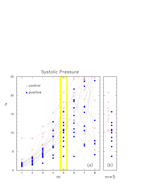
Figure 2: (a) Standard deviations of the wavelet coefficients [Eq. (14)] of the Systolic Pressure in syncope-affected patients (positives) and healthy people (controls). (b) Quite evident separation among positives and controls at $m=5$.

Figure 2(a) shows the scale dependence of the fluctuations (see Eq. (14)) computed for the systolic pressures of our data set. A common trend of $\sigma$’s seems to emerge: the fluctuations of healthy people (open circles) are, at each scale, slightly higher than those of patients with syncope clinical behavior. In particular, a quite clear distinction appears traced in correspondence of the $m=5$ scale value, as can be seen in Fig. 2(b). For smaller values of $m$ there is no sensitive distinction between controls and positives, while, for bigger values our analysis begins to be less and less significant due to the narrowness of our temporal observation window. This distinction is instead lost when a randomly chosen temporal rearrangement of pressure maxima is analysed, as it is shown in Fig. 3.

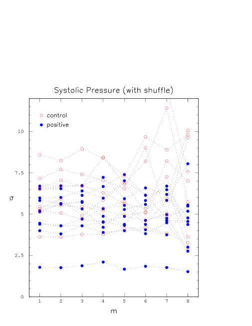
Figure 3: Standard deviations of the wavelet coefficients of the Systolic Pressure computed after a randomly reordering of the pressure wave maxima.

If we interpret this analysis as a possible discriminating test, and if we trace a virtual threshold line in correspondence of $\sigma=12.9$, we observe that the test would have sensitivity of $90\%$ and a specificity of $78\%$. To give a much more quantitative meaning to results of Fig. 2(b) we perform a statistical test: the Wilcoxon-Mann-Whitney (WMW) test [14]. This is aimed to check the hypothesis that our two samples, controls and positives, have been drawn from populations with the same continuous distribution function. The WMW test gives to this hypothesis the $3.5\times 10^{-3}$ probability, i.e. the statistical hypothesis is rejectable at the level of significance of $1\%$.

These empirical observations have been subject of a further study focused to understanding why $m=5$ is the relevant discriminating scale or possibly the onset of a discriminating region between controls and positives. The result of this investigation is that $m=5$ separation corresponds to the fact that positives must have in their Fourier power spectrum, relative to the above-mentioned pressure signal, an “hidden” suppression of a certain low frequency range (roughly centered around $0.02\div 0.03$ Hz, being $m=5$ the resolution window corresponding to about $2^{5}$ pressure maxima). A simple, qualitative, explanation of these results is the following.
If one calculates, with the help of a computer, Haar wavelet coefficients $W_{m,n}$ of a sinus (or cosinus) function using Eq. (12), he will soon realize that what is obtained are derivatives of sinus (or cosinus) rescaled on the $x$-axis. Passing from an $m$ value to the next $m+1$ value, a derivative is made and $x$ units are scaled by a dilation factor $a<1$. This means that, passing from an $m$ to the next, the sinusoidal function will have a greater fluctuation over the zero average value (the area below the curve must remain the same after the rescaling of coordinates). According to what has just been said, a low frequency sinusoidal function, with a small weight coefficient, will start fluctuating in a sensitive way only going up with $m$ values.

Figure 4: Low frequency power spectrum for a control and a positive. A similar behavior holds for all our data records.

As known from Fourier analysis, each function, under very general conditions, can be written down as a sum of weighted sinusoidal functions. If we take two functions differing in their Fourier coefficient values only in a common low frequency range and we calculate their $\sigma(m)$ for different $m$’s, we expect that the function having the smaller weight coefficients in the low frequency domain will also have the smaller $\sigma$ values, for certain particular $m$ values, with respect to the other. For greater $m$’s, the depressed low frequency harmonics begin to fluctuate in a more sensitive way, so that we can foresee again a decreasing in the differences between $\sigma(m)$ values belonging to the two mentioned functions.

In Fig. 4 we show the Fourier power spectrum in the frequency domain of interest. We find the predicted low frequency depression in positives. The Fourier analysed series is again the systolic blood pressure maxima succession. The peaks around $0.05$ Hz which are visible for the displayed control power spectrum are not systematically present in all our controls data set, while the above quoted difference between controls and positives in the $0.02$ Hz range is systematically present in our data records. A Fourier analysis of the entire pressure wave gives a very complicated power spectrum and consequently it is almost impossible to make significant comparisons between positives and controls. Even if this result seems to be encouraging, it has a main drawback. The $m=5$ channel may strictly be connected to the wavelet basis set used and to the particular group of subjects [15]. This at least requires further investigations possibly aimed to highlight features being somehow “universal”, i.e. independent on individuals, but due to the underlying dynamics of the ANS regulation. This is the scope of the next Section.

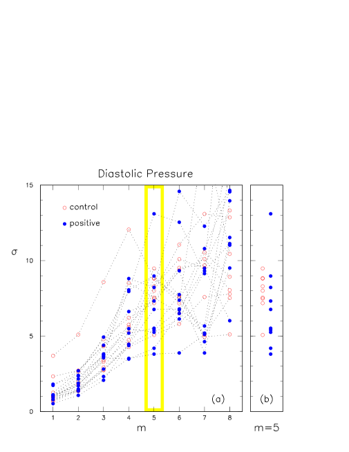
Figure 5: As in Fig. 2 but for the diastolic pressure.

An analysis similar to that carried out for systolic pressure waves has been performed for diastolic pressure waves belonging to the same patients and healthy subjects. As it is shown in Fig. 5(a), a clear evidence for separation between controls and positives is lost even if, at $m=5$ (Fig. 5(b)), controls tend to accumulate towards higher $\sigma$-values than positives. The WMW test, applied to $\sigma$’s in Fig. 5(b), gives now a probability of $8.2\%$. This loss of sensitivity may be due to the shorter variability range of the wavelet coefficients of the diastolic pressures with respect to the systolic ones, as can be extrapolated comparing the vertical scales of Fig. 5 with respect to those in Fig. 2. A physiological grounded understanding of this phenomenon is at the moment lacking.

5 Scale independent measures

With an approach similar to that proposed by [15] we investigate on the possibility to set us free from the $m=5$ discriminating scale in order to find some “universal” features labelling our two distinct classes of subjects. We have calculated the sum $Z_{q}$ of the $q$th moments of the coefficients of the wavelet transform, defined as [2]:

$$Z_{q}(s)=\sum_{n=1}^{L}({\rm max}|W_{s,n}|)^{q},$$ (15)

where $s$ is a continuously varying scale. Wavelet coefficients $W_{s,n}$ are calculated using a formula slightly different from that in Eq. (12):

$$W_{s,n}=\frac{1}{s}\sum_{i=1}^{L}f_{i}\psi\left(\frac{i-n}{s}\right),$$ (16)

where now $n$ ranges in the interval $[1,2,3,...,L]$ and the $\psi$ function is the third derivative of the Gaussian $\psi(x)=\frac{d^{3}}{dx^{3}}e^{-x^{2}/2}$. For a fractal signal $f_{i}$, the following scaling law is expected:

$$Z_{q}(s)\sim s^{\tau(q)}.$$ (17)

A measure of $\tau(q)$, obtained through log-log plots of $Z_{q}(m)$ vs. $m$ for each $q$, could be interpreted as a scale independent measure characterising the unknown underlying dynamics of the ANS regulation of blood pressure. Our goal has been to find out a certain value of $q$ at which appears a significant difference between controls and positives. Using our data record with systolic pressure maxima, we find that the $\tau(q=1)$ acts as a discriminating parameter (see Fig. 6) while with other $q$ values we do not succeed in obtaining equally convincing results. Again we perform a WMW test obtaining a probability of $4.5\times 10^{-3}$ that the two sets of points displayed in Fig. 6 belong to populations with the same continuous distribution function. The same test repeated for the case of diastolic pressures (not shown), gives a probability of $8.3\%$, indicating again a less reliability of this data set for our scopes. Varying the wavelet basis used, we get very different $Z_{q}(s)$ functions. The quoted scaling behavior in Eq. (17) seems possible only if we use, as wavelet basis, the third derivative of the Gaussian. With other bases, such as the Haar basis or the Daubechies one, this scaling is absent. On the other hand a $\sigma(s)$ vs. $s$ plot drawn with $\sigma(s)$ values calculated in Gaussian basis, is completely ineffective to find some separation trend at any $s$ scale.

Figure 6: $\tau(q=1)$ exponents, extracted from our systolic pressure record, are shown.

6 Conclusions and perspectives

We are aware that the analyses here suggested are far to be used as an operative diagnosing method of VS but we show that they strongly suggest some directions to look at. We are not sure that a scale independent measure, such that illustrated in Section 5, can give deeper insights about the problems of VS diagnosis and of understanding the dynamical behavior of ANS than $\sigma(m)$ vs. $m$ plots, illustrated in Section 4. This arises from the fact that the measure described is still linked to the choice of a particular wavelet basis, as is $m$ in the analysis of Section 4. According to us there is a sort of complementarity between the two described approaches which also emerges in the impressive correspondence between results of WMW tests when applied to $\sigma$’s in Haar basis and $\tau$’s in Gaussian basis.

References

- [1] S. Thurner, M.C. Feuerstein, and M.C. Teich, Phys. Rev. Lett. 80, 1544 (1998); Y. Ashkenazy et al., Fractals 6(3), 197 (1998).
- [2] A. Arneodo, Y. d’Aubenton-Carafa, E. Barcy, P.V. Graves, J.F. Muzy, C. Thermes, Physica D 96, 291 (1996).
- [3] H. Kauffman, Neurology 45 (suppl. 5), 12 (1995).
- [4] D.A. Wolfe et al., Am. Fam. Physician 47(1), 149 (1993).
- [5] R. Greger, U. Windhorst, Comprehensive human physiology, ed. Springer-Verlag Berlin Heidelberg 1966, vol. 2, pag. 1995.
- [6] W.N. Kapoor, Cliv. Clin. J. Med. 62(5), 305 (1995).
- [7] G.A. Ruiz et al., Am. Heart J. 130, 345 (1995).
- [8] W.N. Kapoor, Am. J. Med. 97, 78 (1994).
- [9] R.A. Kenny et al., Lancet 14, 1352 (1986).
- [10] B.P. Grubb, D. Kosinski, Current Opinion Cardiology 11, 32 (1996); R. Sheldon et al., Circulation 93, 973 (1996).
- [11] G.A. Ruiz et al., Clin. Cardiol. 19, 215 (1996).
- [12] A. Malliani et al., Circulation 84, 482 (1991).
- [13] R.A. Gopinath et al., Introduction to Wavelets and Wavelet Transforms: a Primer, Prentice Hall 1997; G. Kaiser, A Friendly Guide to Wavelets, Birkhauser 1994; L.Z. Fang, J. Pando, Report astro-ph/9701228, to appear in the Proceedings of the 5th Erice Chalonge School on Astrofundamental Physics, N. Sánchez and A. Zichichi eds., World Scientific, 1997.
- [14] M. Fisz, Probability Theory and Mathematical Statistics, Krieger Publishing Company, 3rd ed., 1980.
- [15] L.S. Nunes Amaral, A.L. Goldberger, P.Ch. Ivanov and H.E. Stanley, Phys. Rev. Lett. 81, 2388 (1998).