High resolution amplitude and phase gratings in atom optics

Abstract

An atom-field geometry is chosen in which an atomic beam traverses a field interaction zone consisting of three fields, one having frequency $\Omega=c/\lambda$ propagating in the ${\bf\hat{z}}$ direction and the other two having frequencies $\Omega+\delta_{1}$ and $\Omega+\delta_{2}$ propagating in the -${\bf\hat{z}}$ direction. For $n_{1}\delta_{1}+n_{2}\delta_{2}=0$ and $\left|\delta_{1}\right|T,\left|\delta_{2}\right|T\gg 1$, where $n_{1}$ and $n_{2}$ are positive integers and $T$ is the pulse duration in the atomic rest frame, the atom-field interaction results in the creation of atom amplitude and phase gratings having period $\lambda/[2(n_{1}+n_{2})]$. In this manner, one can use optical fields having wavelength $\lambda$ to produce atom gratings having periodicity much less than $\lambda$.

03.75.Be, 39.20+q, 32.80.Lg

I Introduction

Over the past several years, atom interferometry has emerged as an important new research area in atomic, molecular and optical physics [1]. The technology has improved to the point where it is now possible to control the center-of-mass motion of atoms using either microfabricated gratings [2] or optical fields [3]. Accompanying the developments in atom interferometry and atom optics have been attempts to produce nanostructures using atom optics elements. Probably the most successful method to date employs standing wave optical fields to focus atoms to a series of lines or dots having size on the order of tens of nanometers [4]. The period of the structures produced in these focusing schemes is $\lambda/2$, where $\lambda$ is the wavelength associated with the standing wave fields. Spatial features having dimensions as small as $\lambda/8$ have been achieved by exploiting the ground state optical potentials for a magnetically degenerate ground state [5], but the period of the entire pattern remains equal to $\lambda/2.$

We have described previously a method for producing spatially modulated atomic densities [6]. When an atomic beam passes through one or more standing wave optical fields having wavelength $\lambda$, it is possible to use coherent transient techniques to create atomic “gratings” having spatial period equal to $\lambda/(2n)$, where $n$ is a positive integer. The atomic gratings arise as a result of the nonlinear interaction between the atoms and the fields. For example, when an atomic beam passes through a resonant, standing wave optical field, the field can create all even spatial harmonics in the excited and ground state populations. As a result of spontaneous emission, the excited state gratings decay back to the ground state; however, for properly chosen level schemes the ground state gratings are not completely ”filled in.” As a consequence, one has long-lived ground state gratings with which to operate. The fate of these ground state gratings depends on the collimation of the atomic beam.

If the angular divergence of the atomic beam is $\theta_{b}$, the gratings persist for a distance of order $L_{b}=\lambda/(2n\theta_{b})$ following the atom-field interaction. For distances larger than $L_{b}$, the gratings wash out quickly as a result of Doppler dephasing. The grating structure is not lost, however. If the atoms interact with a second standing wave field, the various spatial harmonics will rephase at different distances following the interaction with the second field. By a proper choice of optical field strengths, one can create and isolate atomic density patterns that correspond very closely to pure, higher order spatial harmonics [6]. The patterns could be deposited on a substrate and used as elements in soft x-ray systems.

One can also use nonresonant optical fields to interact with the atoms. In this case, one creates a ground state phase grating rather than an amplitude grating [7]. If a highly-collimated atomic beam is used, the phase grating can focus the atoms to a series of lines having spatial period equal to $\lambda/2$. For a beam having angular divergence, echo techniques can be used to rephase and isolate the various spatial harmonics [6, 8].

If the goal of an experiment is to create a pure, higher order spatial harmonic, it would be helpful to eliminate the lower order harmonics from the outset. In this paper, we describe a method in which a single field interaction zone can be used to produce gratings having spatial period equal to $\lambda/(2n)$ where $n\geq 2$ (see Fig. 1). An atomic beam passes through an interaction region in which three fields act. One of the fields has frequency $\Omega$ and propagates in the ${\bf\hat{z}}$ direction, while two additional fields, each counterpropagating relative to the first field, have frequencies $\Omega+\delta_{1}$ and $\Omega+\delta_{2}$, respectively. A two-photon process in which a photon of frequency $\Omega$ is absorbed and one of frequency $\Omega+\delta_{1}$ or $\Omega+\delta_{2}$ is emitted (see Fig. 2a) produces a contribution to the ground state amplitude varying as $e^{2ikz}$, $k=2\pi/\lambda$. Such two-photon processes are not resonant, however, and lead to a vanishingly small second harmonic amplitude if $\left|\delta_{j}T\right|\gg 1$ ($j=1,2)$, where $T$ is the pulse duration in the atomic rest frame. On the other hand, an elementary four-photon process involving the absorption of two photons of frequency $\Omega$ and the emission of one each of frequency $\Omega+\delta_{1}$ and $\Omega+\delta_{2}$ is resonant, provided $\delta_{1}=-\delta_{2}$ (see Fig. 2b). This process is responsible for the creation of the fourth spatial harmonic in the ground state amplitude. Thus the geometry of Fig. 2b can be used to produce a ground state amplitude having spatial period $\lambda/4$ provided $\delta_{1}=-\delta_{2}$. With other choices of $\delta_{1}$ and $\delta_{2},$ one can suppress an arbitrary number of lower order harmonics and produce a ground state amplitude having period $\lambda/(2n)$ where $n>2$.

FIG. 1.: Atom-field geometry. All fields overlap in the interaction region. The detunings $\delta_{1}$ and $\delta_{2}$ are chosen such that $\left|\delta_{1}\right|T,\left|\delta_{2}\right|T\gg 1$, where $T$ is the interaction time in the atomic rest frame.

FIG. 2.: Elementary processes involving fields $E_{0}$, $E_{1}$ and $E_{2}$. (a) Two photon transitions involving field $E_{0}$ and either of fields $E_{1}$ or $E_{2}$ are not resonant (the diagrams are drawn with $\Omega=\omega$). (b) A four photon transition is resonant provided that $\delta_{1}=-\delta_{2}$.

The suppression of lower order harmonics has important implications for nanolithography. It is shown below that the field amplitudes and detunings can be chosen such that a single, higher order atomic grating having period $\lambda/(2n)$ can be created to a high degree of accuracy. Both amplitude and phase gratings can be produced. Phase gratings can lead to atom focusing into lines separated by $\lambda/(2n)\ll\lambda/2$ for $n\gg 1$. Amplitude gratings represent a pure, higher order spatial harmonic that can be deposited on a substrate or used directly to scatter soft x-rays.

Of course, there are other methods for suppressing lower order spatial harmonics. A coherent beam splitter can produce momenta separation of state amplitudes that are greater than $2\hbar k$. As long as these momenta components are not spatially separated, the atomic beam contains density matrix elements in which lower order spatial harmonics are suppressed. Beam splitters based on higher order Bragg scattering [9] can lead to ground state densities corresponding very closely to pure, higher order spatial harmonics. Adiabatic rapid passage [10] can also lead to very nearly pure, higher order spatial harmonics, albeit between state amplitudes corresponding to different internal states. Beam splitters based on triangular optical potentials such as magneto-optical beam splitters [11] and bichromatic beam splitters [12] produce large momenta separations, but not pure spatial harmonics. Our approach is most closely related to that of Yablonovich and Vrijen [13], who use different frequency fields to increase spatial modulation in two-photon microscopy. Here we extend and expand their ideas to the domain of atom optics and atom interferometry.

The paper is organized as follows: In Section II, an illustrative example is considered in which the second order spatial harmonic is suppressed. Methods for creating both amplitude and phase gratings are discussed, as are the effects of spontaneous decay during the pulse. Both numerical solutions and an approximate analytical solution is considered in this section. In Sec. III, numerical solutions are presented for the suppression of harmonics beyond second order. It is shown that high contrast, amplitude gratings can be created for arbitrary $n$. A summary of the results is given in Sec. IV, and the implications for nanolithography are discussed.

II Illustrative Example

Many of the features of harmonic suppression can be illustrated for the field geometry of Fig. 1. The atomic beam propagates in the ${\bf\hat{x}}$ direction and the fields propagate along the z-axis. The total field can be written as ${\bf E}({\bf r},t)={\bf E}(z,t)f(x,y),$ where $f(x,y)$ is a spatial mode function,

$${\bf E}(z,t) = \frac{1}{2}\widehat{{\bf y}}\left[E_{0}e^{i(kz-\Omega t)}+E_{1}e^{i[-kz-(\Omega+\delta_{1})t]}\right.$$ (2)

$$+\left.E_{2}e^{i[-kz-(\Omega+\delta_{2})t]}\right]+c.c.,$$

and $c.c$. stands for complex conjugate. Fields 1 and 2 propagate in the -${\bf\hat{z}}$ direction and field 0 in the +${\bf\hat{z}}$ direction. In this section, we set $E_{1}=E_{2}$, take $E_{1}$ and $E_{0}$ to be real, and set $\delta_{1}=-\delta_{2}\equiv\delta$, such that

$${\bf E}(z,t)=\frac{1}{2}\widehat{{\bf y}}e^{-i\Omega t}\left[E_{0}e^{ikz}+2E_{1}e^{-ikz}\cos(\delta t)\right]+c.c.$$ (3)

In the atomic rest frame these fields appear as a radiation pulse and the field amplitudes become functions of time. The atoms are modeled as having two levels, 1 and 2, separated in frequency by $\omega.$ The problem divides into two parts, interaction of the atoms with the fields and free evolution of the atoms following the field interaction. In the main body of the paper we consider only the field interaction region. In the field interaction region, all effects associated with quantization of the atoms’ center-of-mass motion, as well as any transverse Doppler shifts, are neglected. In Sec. IV, we will discuss the free evolution of the atoms following their interaction with the field.

In the atomic rest frame, the state amplitudes $a_{1}$ and $a_{2}$ evolve as

$${\bf\dot{a}=}-i{\bf F(}z,t){\bf a}-2i{\bf G(}z,t{\bf)a},$$ (4)

where

$${\bf a} = \left(\begin{array}[]{c}a_{1}\\ a_{2}\end{array}\right);$$ (7)

$${\bf F(}z,t) = \left(\begin{array}[]{cc}\Delta/2&\chi_{0}(z,t)^{\ast}\\ \chi_{0}(z,t)&-\Delta/2\end{array}\right);$$ (10)

$${\bf G}(z,t) = \left(\begin{array}[]{cc}0&\chi_{1}(z,t)^{\ast}\\ \chi_{1}(z,t)&0\end{array}\right)\cos(\delta t),$$ (13)

$\chi_{0}(z,t)$ and $\chi_{1}(z,t)$ are Rabi frequencies defined by

$$\chi_{j}(z,t) = \chi_{j}(t)e^{ik_{j}z};$$ (14)

$$\chi_{j}(t) = -\mu E_{j}(t)/2\hbar=[\chi_{j}(t)]^{\ast}\geq 0;\text{ \{}j=0,1,2\};$$ (15)

$$k_{0} = -k_{1}=-k_{2}=k,$$ (16)

$\Delta=\Omega-\omega$ is an atom-field detuning, $\mu$ is a dipole moment matrix element, and $E_{j}(t)$ is a pulse envelope function in the atomic rest frame. Spontaneous decay during the pulse has been neglected for the moment. Equation (4) can be solved numerically for any pulse envelopes $E_{j}(t)$. The advantage of the choice of parameters considered in this section is that they allow for a very good approximate analytical solution that illustrates the relevant physical concepts.

Since the two matrix elements of ${\bf G}$ have the same time dependence, it is convenient to write a solution to Eq. (4) in the form

$${\bf a(}t) = {\bf S}(z,t)\,{\bf\tilde{a}(}t);$$ (18)

$${\bf S}(z,t) = \exp\left\{-2i\int_{-\infty}^{t}{\bf G}(z,t^{\prime})dt^{\prime}\right\}$$ (19)

where the matrix ${\bf\tilde{a}(}t)$ satisfies the differential equation

$$d{\bf\tilde{a}/}dt=-i{\bf S}^{\dagger}{\bf(}z,t){\bf F(}z,t{\bf)S(}z,t{\bf)\tilde{a}.}$$ (20)

For a smoothly varying pulse having duration $T\gg$ $\delta^{-1}$, the integral in Eq. (19) can be evaluated asymptotically. It follows that

$${\bf S(}z,t{\bf)} \sim {\bf\exp}\left\{-2i\frac{\sin(\delta t)}{\delta}\left(\begin{array}[]{cc}0&\chi_{1}(z,t)^{\ast}\\ \chi_{1}(z,t)&0\end{array}\right)\right\}$$ (23)

$$= \cos(\theta)\,{\bf 1}-i\,\sin(\theta)\left(\begin{array}[]{cc}0&e^{ikz}\\ e^{-ikz}&0\end{array}\right),$$ (26)

where

$$\theta=2\chi_{1}(t)\sin(\delta t)/\delta,$$ (27)

1 is the unit matrix, and we have used the fact that $\chi_{1}(z,t)/\left|\chi_{1}(z,t)\right|=\exp(-ikz)$. The S-matrix reduces to the unit matrix as $t\sim\pm\infty.$ Combining Eqs. (II)- (27), one finds

$$d{\bf\tilde{a}/}dt = -i\frac{\Delta}{2}{\bf\cos(}2\theta)\left(\begin{array}[]{cc}1&0\\ 0&-1\end{array}\right){\bf\tilde{a}}-i\left(\begin{array}[]{cc}0&M\\ M^{\ast}&0\end{array}\right){\bf\tilde{a}}$$ (35)

$${\bf+}\frac{\sin(2\theta)}{2}\left(\begin{array}[]{cc}N&-\Delta e^{ikz}\\ \Delta e^{-ikz}&N^{\ast}\end{array}\right){\bf\tilde{a}}$$

where

$$M = \chi_{0}(t)\left[\cos^{2}(\theta)e^{-ikz}+\sin^{2}(\theta)e^{3ikz}\right];$$ (37)

$$N = 2i\chi_{0}(t)\sin(2kz).$$ (38)

Equation (35) can be simplified considerably if

$$\delta\gg\chi_{0}(t),\text{ }\Delta,\text{ }\chi_{0}(t)\chi_{1}^{2}(t)/\delta^{2}.$$ (39)

In that limit, it is possible to ”course-grain” Eq. (35) on a time scale greater than $\delta^{-1}$ and replace all trigonometric functions appearing in Eqs. (35) and (II) by their time averages. Using Bessel function expansions for the trigonometric functions, one finds

$$\alpha \equiv \overline{\cos^{2}(\theta)}=\frac{1+J_{0}[4\chi_{1}(t)/\delta]}{2};$$ (40)

$$\beta \equiv \overline{\sin^{2}(\theta)}=\frac{1-J_{0}[4\chi_{1}(t)/\delta]}{2};\qquad\overline{\sin(2\theta)}=0,$$ (41)

where $J_{0}$ is a Bessel function and the bar indicates a time average. In this limit, Eq. (35) is replaced by

$$d{\bf\tilde{a}/}dt = -i\frac{\Delta}{2}J_{0}[4\chi_{1}(t)/\delta]\left(\begin{array}[]{cc}1&0\\ 0&-1\end{array}\right){\bf\tilde{a}}$$ (47)

$$-i\chi_{0}(t)\left(\begin{array}[]{cc}0&\alpha e^{-ikz}+\beta e^{3ikz}\\ \alpha e^{ikz}+\beta e^{-3ikz}&0\end{array}\right){\bf\tilde{a}.}$$

Equation (47) admits solutions which represent both amplitude and phase gratings in the ground state atomic density. We examine these cases separately.

A Amplitude gratings  $\Delta=0$

It is possible to obtain amplitude gratings having maximum contrast for the ground and excited state populations by choosing $\Delta=0$ ($\Omega=\omega).$ In this limit, Eq. (47) reduces to

$$d{\bf\tilde{a}/}dt=-i\chi_{0}(t)\left(\begin{array}[]{cc}0&\alpha e^{-ikz}+\beta e^{3ikz}\\ \alpha e^{ikz}+\beta e^{-3ikz}&0\end{array}\right){\bf\tilde{a}.}$$ (48)

It will prove useful to look at the perturbative limit of Eq. (48). When $\chi_{1}(t)/\delta\ll 1,$ the time evolution of state 2 is

$$d\tilde{a}_{2}{\bf/}dt=-i\chi_{0}(t)e^{ikz}\tilde{a}_{1}-2i\frac{\chi_{0}(t)[\chi_{1}(t)]^{2}}{\delta^{2}}e^{-3ikz}\tilde{a}_{1}.$$ (49)

The fundamental processes responsible for excitation to state 2 from state 1 are shown schematically in Fig. 3. There can be direct, resonant excitation to state 2 by field $E_{0}$ and three-photon, resonant excitation involving the absorption of one photon each from fields $E_{1}$ and $E_{2}$ and emission of one photon into field $E_{0}$ (as noted above, the amplitude modulated field used in this section can be considered as a sum of two fields having frequencies $\Omega_{1}=\Omega+\delta_{1}$ and $\Omega_{2}=\Omega+\delta_{2}$, with $\delta_{1}=-\delta_{2}\equiv\delta$). The three-photon processes are resonant since $\Omega_{1}+$ $\Omega_{2}-\Omega=\omega$ when $\Omega=\omega$. In these diagrams, the Rabi frequency $\chi_{0}$ is a shorthand notation for $\chi_{0}(z,t)$ and contains a factor $e^{ikz}$ and, similarly, Rabi frequencies $\chi_{1}$ and $\chi_{2}$ contain factors $e^{-ikz}$. The overall amplitude for the one photon process varies as $\chi_{0}e^{ikz}$ and as ($\chi_{0}\chi_{1}\chi_{2})e^{-3ikz}/\delta^{2}$ for the three-photon processes. The $\delta^{2}$ factor reflects the fact that the two intermediate states in the three-photon processes are each off-resonance by an energy $\hbar\delta$. In taking the square of the amplitude, one finds a spatial modulation at $4kz.$ As seen in Sec. III, diagrams of this type can be used to estimate the required field strengths for suppression of higher order harmonics.

FIG. 3.: Elementary processes leading to the resonant excitation of state 2. The Rabi frequencies $\chi_{j}$ are a shorthand notation for $\chi_{j}(z,t)$ and contain spatial phase factors. In forming the upper state probability, interference terms lead to a spatial modulation having period $\lambda/4$.

Equation (48) cannot be solved analytically for arbitrary pulse envelope functions. On the other hand, it can be solved analytically if we assume square pulses, $E_{j}(t)=E_{j}$ for $0\leq t\leq T$ and zero otherwise. [Equation (27) remains valid for a square pulse. Moreover, if one chooses a detuning $\delta T=n\pi$, then the S-matrix in Eq. (26) reduces to the unit matrix at the beginning and end of the pulse. Thus one can use Eq. (48), even though a square pulse does not satisfy the adiabaticity conditions at turn on and turn off.] For a square pulse, one finds

$$\left|a_{2}(T)\right|^{2} = \left|\tilde{a}_{2}(T)\right|^{2}=\sin^{2}\left[\chi_{0}T\left|\alpha e^{-ikz}+\beta e^{3ikz}\right|\right]$$ (50)

$$= \sin^{2}\left\{\chi_{0}T\left(\left[(1+J_{0}^{2}\{4\chi_{1}/\delta\})\right.\right.\right.$$ (52)

$$\left.\left.\left.+(1-J_{0}^{2}\{4\chi_{1}/\delta\})\cos 4kz\right]/2\right)^{1/2}\right\}.$$

It follows from Eq. (52) [or from Eq. (48)] that the excited state population immediately after the pulse is a periodic function of $z$ having period $\lambda/4$. The second order spatial harmonic having period $\lambda/2$ has been $\sup$pressed, owing to the large detunings $\pm\delta$ of the fields propagating in the $-{\bf\hat{z}}$ direction. By taking a field strength corresponding to the first zero of the Bessel function $J_{0}[4\chi_{1}/\delta]$ ($\chi_{1}\sim 0.6\delta)$, one can optimize the grating contrast for the smallest possible value of $\chi_{0}T$. If $J_{0}[4\chi_{1}/\delta]=0,$ then $\left|a_{2}(T)\right|^{2}=\sin^{2}\left[\chi_{0}T\cos(2kz)\right]$. This function is plotted as a function of $kz$ in Fig. 4 for several values of $\chi_{0}T$.

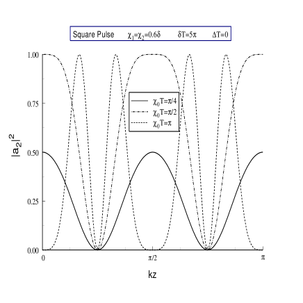
FIG. 4.: Graphs of the upper state probability as a function of $kz$ for excitation by a rectangular pulse, with $\delta_{1}=-\delta_{2}\equiv\delta$.

For values of $\chi_{0}T\ll\pi/2$, the grating contrast in the excited state amplitude is less than unity, but the grating is close to pure fourth harmonic. For $\chi_{0}T\geq\pi/2$, the grating contrast is always unity, but harmonics higher than fourth are evident. A choice of pulse area that leads to high grating contrast while producing a spatial distribution very close to pure fourth harmonic is $\chi_{0}T=1.3$, for which the Bessel function expansion of $\sin^{2}\left[\chi_{0}T\cos(2kz)\right]$ yields

$$\left|a_{2}(T)\right|^{2} \sim \left[1-J_{0}(2.6)+J_{2}(2.6)\cos(4kz)\right.$$ (54)

$$\left.-J_{4}(2.6)\cos(8kz)+\ldots\right]/2$$

$$\approx [1.1+0.92\cos(4kz)-0.17\cos(8kz)]/2.$$ (55)

This grating has a fringe contrast of 0.93 and consists primarily of fourth harmonic.

The qualitative results do not change when smooth pulses are used. The original differential equation (13) was solved numerically for Gaussian pulses,

$$\chi_{j}(t)=\chi_{j}e^{-(t/T)^{2}}/\sqrt{\pi}.$$ (56)

From this point onward, we set $T=1$ and evaluate all times in units of $T$ and all frequencies in units of $T^{-1}$. In these units, the quantity $2\chi_{j}$ corresponds to the area of pulse $j$. In all the examples, $\delta\geq 3$, which, for the Gaussian pulse (56), is sufficient to guarantee adiabaticity, provided that conditions (39) are also met.

In Fig. 5, the solutions of the exact equations [Eq. (13)] for the upper state probability are compared with those of the coarse-grained equations [Eq. (48)]. Recall that the solutions of the course grained equations should approach those of the exact equations as the ratio $\delta/\chi_{0}$ increases. This feature is seen clearly in Fig. 5. The curve having $\delta/\chi_{0}=40$ correspond to the solution of both the exact and course-grained equations - they are not distinguishable for this ratio of $\delta/\chi_{0}.$ Even for $\delta/\chi_{0}=5,$ the results do not differ by much.

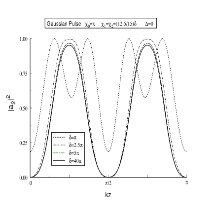
FIG. 5.: Graphs of the upper state probability as a function of $kz$ for excitation by a Gaussian pulse, with $\delta_{1}=-\delta_{2}\equiv\delta$. In this and subsequent graphs, all frequencies are in units of $T^{-1}$. With increasing ratio of $\delta/\chi_{0}$, the solution of the exact equations (13) approaches that of the course-grained equations (49), represented by the solid line in the plot.

The course grained equations depend only on the parameters $\chi_{0}$ and $\delta/\chi_{1}$; consequently the solutions of the exact equations depend on these two parameters only for $\delta/\chi_{0}\gg 1$. If $\delta/\chi_{0}\lesssim 1$, the solution of the exact equations depends independently on the parameters $\chi_{0},$ $\delta$, and $\chi_{1}$; moreover, the solution has period $\lambda/2$ rather than $\lambda/4$. Although not evident from the figure, the $\delta=\chi_{0}$ results differ from pure $\lambda/4$ periodicity by as much as 10%. These differences are more evident in Fig. 6, drawn for $\delta/\chi_{0}=1/3$. To assure $\lambda/4$ periodicity, one must have $\delta/\chi_{0}\gtrsim 5$.

FIG. 6.: Graphs of the upper state probability as a function of $kz$ for excitation by a Gaussian pulse, with $\delta_{1}=-\delta_{2}\equiv\delta$ and $\delta/\chi_{0}=1/3$. For this ratio, the ”course-graining” approximation is no longer valid and the period of the amplitude grating is $\lambda/2$ rather than $\lambda/4$.

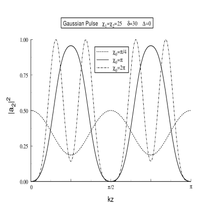
FIG. 7.: Graphs of the upper state probability as a function of $kz$ for excitation by a Gaussian pulse, with $\delta_{1}=-\delta_{2}\equiv\delta$ and several values of $\chi_{0}$.

In Fig. 7, the upper state probability is plotted as a function of $kz$ for fixed $\chi_{1}/\delta=5/6$, and several values of $\chi_{0}$. These curves follow the same qualitative behavior as those shown in Fig. 4 for the square pulse. In Fig. 8, the upper state probability is plotted as a function of $kz$ for fixed $\chi_{0}=\pi$ and several values of $\chi_{1}/\delta$. For $\chi_{1}/\delta\lesssim 0.5$, the grating contrast is less than unity, but the grating is very nearly pure fourth harmonic. With increasing $\chi_{1}/\delta$, the grating contrast approaches unity and harmonics of order ($4+4n)$, $n\geq 1$, are evident.

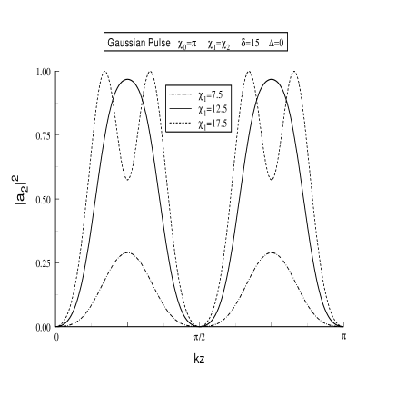
FIG. 8.: Graphs of the upper state probability as a function of $kz$ for excitation by a Gaussian pulse, with $\delta_{1}=-\delta_{2}\equiv\delta$ and several values of $\chi_{1}$.

B Phase Gratings  $\Delta>1$

When $\Delta>1$, the elementary processes shown in Fig. 3 are no longer resonant. Thus one expects that the excited state population following the pulse to be negligible. On the other hand the resonant, elementary 4-photon processes, shown in Fig. 9, lead to a modification of the phase of the ground state amplitude.

FIG. 9.: Elementary processes leading to a phase grating in the ground state amplitude. The second and third diagrams in the figure are spatially modulated with period $\lambda/4$.

To calculate the phase change of the ground state amplitude, it is convenient to use the semiclassical dressed states associated with Eq. (48). These states are obtained by instantaneously diagonalizing Eq. (48). If

$$\Delta^{2}J_{0}^{2}\left\{\frac{4\chi_{1}(t)}{\delta}\right\}$$ (57)

$$+2\chi_{0}(t)^{2}\left\{\left(1+J_{0}^{2}\left\{\frac{4\chi_{1}(t)}{\delta}\right\}\right)\right.$$ (58)

$$+\left.\left(1-J_{0}^{2}\left\{\frac{4\chi_{1}(t)}{\delta}\right\}\right)\cos 4kz\right\}\left.\gg 1\right.$$ (59)

the system remains in the instantaneous eigenstate that evolves from the ground state as the field is turned on and returns to the ground state following the pulse. The net phase change is simply the integral of the dressed state energy divided by $\hbar.$ Explicitly, one finds.

$$a_{1}(\infty)=e^{-i\phi},$$ (60)

where

$$\phi = \frac{1}{2}\int_{-\infty}^{\infty}dt\left\{\Delta^{2}J_{0}^{2}\left\{\frac{4\chi_{1}(t)}{\delta}\right\}\right.$$ (63)

$$+2\chi_{0}(t)^{2}\left[\left(1+J_{0}^{2}\left\{\frac{4\chi_{1}(t)}{\delta}\right\}\right)\right.$$

$$+\left.\left.\left(1-J_{0}^{2}\left\{\frac{4\chi_{1}(t)}{\delta}\right\}\right)\cos 4kz\right]\right\}^{1/2}$$

For Gaussian pulses (56), the phase $\phi$ is plotted as a function of $kz$ in Fig. 10 for several values of $\chi_{0},$ $\chi_{1}$, $\delta$, and $\Delta$.

FIG. 10.: Graphs of the ground state phase as a function of $kz$ for excitation by a Gaussian pulse, with $\delta_{1}=-\delta_{2}\equiv\delta$. The solid lines are a solution of the exact equations while the dashed lines are obtained from the course-grained, dressed state equations.

The solid line represents solutions of the exact equations (13) and the dotted line the values given by Eq. (63), with the phase arbitrarily taken equal to zero at $kz=0$. The results agree when conditions (59) and (39) are satisfied. For $\chi_{1}/\delta\geq 0.6$, there are times during the atom-field interaction for which $J_{0}\left\{\frac{4\chi_{1}(t)}{\delta}\right\}=0.$ As a consequence, condition (59) is violated near $kz=\pi/4$ and $3\pi/4$. This explains the small deviations between the exact and approximate solutions for these values of $kz$. For all cases shown, $\left|a_{1}(\infty)\right|\sim 1$. It is seen that significant phase modulation of the ground state can be achieved with suppression of the second spatial harmonic.

A necessary condition for significant spatial modulation of the phase is $\chi_{0}\chi_{1}^{2}/\delta^{2}\geq 1$. If $\Delta^{2}J_{0}^{2}\left\{\frac{4\chi_{1}(t)}{\delta}\right\}\ll\chi_{0}(t)^{2}$, then the effective pulse area for the creation of the phase grating is of order $\chi_{0},$ while it is of order $\chi_{0}^{2}/\Delta$ for $\Delta^{2}J_{0}^{2}\left\{\frac{4\chi_{1}(t)}{\delta}\right\}\gg\chi_{0}(t)^{2}$.

C Role of Spontaneous Emission

So far we have neglected the role of spontaneous emission during the excitation pulse. To investigate the role of spontaneous emission during the pulse, we adopt a highly simplified decay scheme in which state 2 decays to a state outside the two-state manifold with rate 2$\gamma$. As a result, population leaks out of the two-level manifold. Clearly, any excited state amplitude grating will be diminished by decay. It also turns out that phase gratings are destroyed by spontaneous decay since the excited state population during the pulse is not negligible under conditions favoring a significant spatially modulated phase grating. Spontaneous emission breaks the adiabatic following that would return the atom to its ground state in the absence of such decay [14].

Within the context of this model, spontaneous emission can be included in Eq. (13) by the addition of a term

$\displaystyle-\gamma\left(\begin{array}[]{cc}0&0\\ 0&1\end{array}\right){\bf a}.$

This decay term results in an addition to Eq. (48) of the form

$\displaystyle-\gamma\left(\begin{array}[]{cc}\frac{1-J_{0}[4\chi_{1}(t)/\delta]}{2}&0\\ 0&\frac{1+J_{0}[4\chi_{1}(t)/\delta]}{2}\end{array}\right){\bf\tilde{a}}.$

For any nonvanishing field strength $\chi_{1}$, both dressed state amplitudes $\tilde{a}_{1}$ and $\tilde{a}_{2}$ decay. For the field strength giving rise to maximum spatial modulation, $J_{0}[4\chi_{1}(t)/\delta]\sim 0$, spontaneous emission destroys grating formation when $\gamma\gtrsim 1$. This is easily understood. To have strong spatial modulation of amplitude or phase gratings, there is always a significant excited state population during the pulse; any decay results in a loss of population from the system in our simple decay scheme.

We have also carried out density matrix calculations using various decay schemes. It appears that one must require $\gamma\lesssim 0.5$ to retain reasonable grating contrast.

III Suppression of Higher Order Harmonics

One can generalize the previous results to allow for the suppression of harmonics higher than second order. The appropriate field geometry is shown in Fig. 1. Spontaneous emission during the atom-pulse interaction is neglected. For the field (2), the state amplitudes evolve as

$${\bf\dot{a}=}-i{\bf F(}z,t){\bf a}-i{\bf H(}z,t{\bf)a}$$ (64)

where ${\bf F(}z,t)$ is defined by (13) and

$${\bf H}(z,t)=\left(\begin{array}[]{cc}0&\begin{array}[]{c}\chi_{1}(z,t)^{\ast}e^{i\delta_{1}t}\\ +\chi_{2}(z,t)^{\ast}e^{i\delta_{2}t}\end{array}\\ \begin{array}[]{c}\chi_{1}(z,t)e^{-i\delta_{1}t}\\ +\chi_{2}(z,t)e^{-i\delta_{2}t}\end{array}&0\end{array}\right).$$ (65)

Since ${\bf H}(z,t)$ cannot be factored as a constant matrix times a function of $t$, the method used in Sec. II is not applicable. On the other hand it is not difficult to obtain numerical solutions of Eq. (65).

Diagrams similar to those shown in Figs. 3 and 9 can help us to estimate the field strengths needed to obtain both amplitude and phase gratings. Before considering such diagrams, we note that the lowest order ac Stark shift,

$$\xi=\left(\chi_{1}^{2}/\delta_{1}+\chi_{2}^{2}/\delta_{2}\right)$$ (66)

no longer vanishes automatically as it does for an amplitude modulated field ($\chi_{1}=\chi_{2};\quad\delta_{1}=-\delta_{2})$. To suppress the higher order harmonics, it is necessary that $\left|\delta_{1}\right|$ and $\left|\delta_{2}\right|$ be large compared with all characteristic frequencies in the problems, including the ac Stark shifts. In order to have $\left|\delta_{1}\right|,\left|\delta_{2}\right|>\xi$, it is necessary that $\chi_{1}^{2}/\delta_{1}^{2}\ll 1$, $\chi_{2}^{2}/\delta_{2}^{2}\ll 1$, unless $\delta_{1}$ and $\delta_{2}$ have opposite signs and the field strengths are chosen such that

$$\left(\chi_{1}^{2}/\delta_{1}+\chi_{2}^{2}/\delta_{2}\right)=0.$$ (67)

In this case it is possible to have $\chi_{1}\sim\delta_{1}$ and still have $\left|\delta_{1}\right|,\left|\delta_{2}\right|>\xi$. Since it is necessary to have $\chi_{1}\sim\delta_{1}$ for significant spatial modulation in the state populations, it is important to choose the Rabi frequencies such that Eq. (67) is satisfied. Higher order contributions to the ac Stark effect may still play a role. From the numerical solutions, it appears that one must choose $\chi_{1}$ and $\chi_{2}$ less than or of order $\left|\delta_{1}\right|$,$\left|\delta_{2}\right|,$ to obtain the desired periodicity.

The elementary processes giving rise to an amplitude grating are illustrated in Fig. 11. The grating is formed by terms representing the interference of the two diagrams shown in the figure.

FIG. 11.: Elementary processes leading to the resonant excitation of state 2 and suppression of spatial harmonics higher than fourth. The detunings are chosen such that $n_{1}\delta_{1}+n_{2}\delta_{2}=0,$ leading to an amplitude grating having period $\lambda/[2(n_{1}+n_{2})]$.

The resonance condition for the second diagram is

$$n_{1}\delta_{1}+n_{2}\delta_{2}=0$$ (68)

when $\Delta=0$ and the integers $n_{1}>$ $n_{2}$ contain no common factors. The lowest order nonvanishing harmonic varies as cos[2($n_{1}+n_{2})kz]$. The amplitude associated with this harmonic is of order

$$A(n_{1},n_{2})=\frac{\chi_{0}^{n_{1}+n_{2}}\chi_{1}^{n_{1}}\chi_{2}^{n_{2}}}{\delta^{2(n_{1}+n_{2}-1)}},$$ (69)

where $\delta$ is of order $\left|\delta_{1}\right|$ or $\left|\delta_{2}\right|$. To obtain good grating contrast, one requires that

$$A(n_{1},n_{2})\sim 1\text{.}$$ (70)

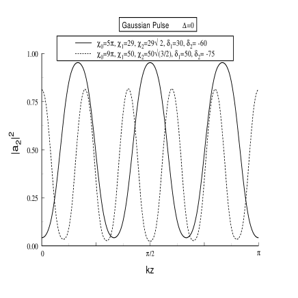
FIG. 12.: Graphs of the upper state probability as a function of $kz$ for excitation by a Gaussian pulse, with $n_{1}\delta_{1}+n_{2}\delta_{2}=0.$ Graphs are shown for ($n_{1}=2$, $n_{2}=1$) (sixth harmonic) and ($n_{1}=3$, $n_{2}=2$) (tenth harmonic).

Condition (70) can be satisfied if $\chi_{0}\sim\delta^{1-2/(n_{1}+n_{2})}$, but, to suppress lower harmonics, it is also necessary that $\chi_{0}\ll\delta$. As ($n_{1}+n_{2})$ increases, $\delta$ and $\chi_{0}$ must be taken larger and larger to simultaneously satisfy these conditions.

In Fig. 12 the upper state population is plotted as a function of $kz$ for ($n_{1}=2$, $n_{2}=1$) (sixth harmonic) and for ($n_{1}=3$, $n_{2}=2$) (tenth harmonic). The field strengths are chosen such that $\chi_{2}=\sqrt{n_{1}/n_{2}}\chi_{1}$ according to Eqs. (67) and (68), and $\chi_{1}$ is taken to be of order $\delta_{1}$. It is seen that amplitude gratings having periods as small as $\lambda/10$ can be produced with contrast of order unity. For sufficiently large $\delta$, an arbitrary number of lower order harmonics can be suppressed.

FIG. 13.: Elementary processes leading to a ground state phase grating and suppression of spatial harmonics higher than fourth. The detunings are chosen such that. $n_{1}\delta_{1}+n_{2}\delta_{2}=0,$ leading to a phase grating having period $\lambda/[2(n_{1}+n_{2})]$.

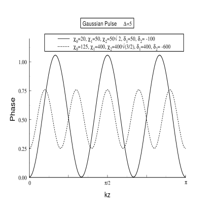
FIG. 14.: Graphs of the ground state phase as a function of $kz$ for excitation by a Gaussian pulse, with $n_{1}\delta_{1}+n_{2}\delta_{2}=0.$ Graphs are shown for ($n_{1}=2$, $n_{2}=1$) (sixth harmonic) and ($n_{1}=3$, $n_{2}=2$) (tenth harmonic).

The conditions for producing phase gratings are similar, but a little more severe, than those for producing amplitude gratings, provided one takes $\Delta>1$, but $\chi_{0}\gg\Delta.$ The elementary processes giving rise to an phase grating are illustrated in Fig. 13. The highest contrast phase gratings are produced when $A(n_{1},n_{2})\sim\Delta$, which can be satisfied if $\chi_{0}\sim\delta^{1-2/(n_{1}+n_{2})}\Delta^{1/(n_{1}+n_{2})}$. Along with the requirement that $\chi_{0}\ll\delta$, this condition implies that large values of $\delta$ and $\chi_{0}$ are needed to produce large phase gratings as ($n_{1}+n_{2})$ increases. The phase of the ground state amplitude is shown as a function of $kz$ in Fig. 14 for ($n_{1}=2$, $n_{1}=1$) (sixth harmonic) and for ($n_{1}=3$, $n_{2}=2$) (tenth harmonic). In all cases shown, $\left|a_{1}(\infty)\right|\sim 1$ . Clearly it is also possible to produce phase gratings having reasonable contrast with the suppression of lower order harmonics.

IV Discussion

It has been shown that atom-field interactions can be used to create high contrast amplitude gratings for atomic state populations and phase gratings for atomic ground state amplitudes. If counterpropagating fields having wavelength $\lambda$ are used, it is possible to choose atom-field detunings such that the lowest spatial harmonic component in the gratings has period $\lambda/2n$, where $n$ is an integer. For the sake of definiteness, we will refer to the harmonic having period $\lambda/2n$ as the (2$n)$th harmonic. The gratings produced are not pure in the sense that they contain all integer multiples of the (2$n)$th harmonic, but the field strengths can be chosen in such a manner as to maximize the contribution from the (2$n)$th harmonic. Once the gratings are created, the question remains as how to image the gratings at some distance $L$ from the atom-field interaction zone. One can probe the gratings by applying counterpropagating fields having frequencies $\Omega$ and $\Omega+\delta_{1}$ to generate a signal with frequency $\Omega+\delta_{2}$; alternatively, one can deposit the atomic density grating on a substrate. The situation is different for amplitude and phase gratings.

In the case of amplitude gratings, one has the option of working with distances $L$ that correspond to either classical or quantum-mechanical scattering for the atoms. If $L\gtrsim L_{T},$ where the so-called Talbot length $L_{T}$ is defined by $L_{T}=2(\lambda/2n)^{2}/\lambda_{dB}$ ($\lambda_{dB}$ is the atomic de Broglie wavelength), the atomic center-of-mass motion for the atoms must be treated quantum mechanically; for $L\ll L_{T}$, this motion can be treated classically. Typically, $L_{T}$ is of order of a few cm for a thermal beam. We restrict our discussion to the classical scattering limit. For classical scattering, the total atomic density is not modulated, as long as no state-selective mechanism removes atoms from the system. In other words, the excited and ground state population can be modulated following interaction with the fields, but the sum of these populations is not modified. If the excited state population decays to the ground state following interaction with the field, the grating structure disappears. There are several methods to maintain the gratings following the atom-field interaction. The most direct method is to use optical transitions, such as those in Ca, Mg, or Yb, with lifetimes approaching a microsecond or longer. One can then probe the population difference grating following the atom-field interaction or selectively ionize excited state atoms to leave a net atomic density grating that could be deposited on a substrate.

For shorter-lived atomic transitions, there are several alternatives. One possibility is to ionize some of the excited state atoms during the atom-field interaction, which would leave a net atomic density grating. Another possibility is to use atoms whose ground state consists of a manifold of substates. When the excited state decays, the total ground state density is not modulated, but that of specific substates may be modulated. By selectively ionizing some of the ground state sublevels, one again achieves a net atomic density grating. Still another alternative is to use a beam of metastable atoms and drive transitions between the metastable state and an excited state that can decay back to the ground state [15]. Following the atom-field interaction, there will be a grating of metastable atoms that can be detected selectively.

In the case of shorter-lived excited states, one can run into problems related to the effective pulse interaction time $T$ which corresponds to the transit time of the atoms through the field interaction zone. Recall that all frequencies are measured in units of $T^{-1}$. For appreciable gratings, it is necessary that $\gamma T\lesssim 0.5$. If the fields are focused to a spot size of 10 $\mu$ and the longitudinal atomic speed is $5\times 10^{4}$ cm/s, then $T\approx 20$ ns. For these parameters, one must use atoms whose excited state lifetime exceeds 20 ns. It is also possible to limit the atom-field interaction time by using pulsed fields. For transit times of order 20 ns, the detunings and Rabi field strengths considered in this paper correspond to frequencies in the MHz to GHz range. Such values do not pose any serious experimental difficulties.

Assuming that we can produce a density grating, many methods are available for imaging the gratings. Perhaps the most direct method is to detect the grating immediately following the atom-field interaction. This scheme is analogous to free-induction decay (FID) in coherent transient spectroscopy. All harmonics in the beam are superimposed, and the grating begins to wash out as a result of the transverse Doppler effect at distances $L_{b}=\lambda/(2n\theta_{b})$, where $\theta_{b}$ is the atomic beam divergence. To avoid overlap of the different harmonic components, echo techniques can be used [16]. With two interaction zones separated by a distance $L_{0},$ different harmonics are focused at different distances following the second interaction zone. For example, one can optimize the $(2n)$th harmonic at $L=2L_{0}$, the $(4n)$th harmonic at $L=3L_{0}/2,$ the $(6n)$th harmonic at $L=4L_{0}/3$, etc. In this manner one is able to isolate and focus harmonics higher than $2n$ which were created in the first field interaction zone [6]. For example, one could create 4th harmonic in the first interaction zone and 16th harmonic in the second interaction zone to optimize the $12$th harmonic at $L=4L_{0}/3$.

Although FID and echo techniques can be used also for phase gratings [8], we consider here only the focusing capabilities of phase gratings. The phase grating can be thought to arise as the result of an ac Stark shift potential that acts as a spatially modulated index of refraction for the atoms and causes them to focus at a distance of order $L_{T}/A$, where $A$ is some effective pulse area in the problem associated with the creation of the $\left(2n\right)$th harmonic. In this manner, one can focus an atomic beam to a series of lines (or dots if a 2-D geometry is utilized) having spacing $\lambda/2n$.

In summary, we have outlined methods for generating and detecting spatially modulated atomic density amplitude or phase gratings having period $\lambda/2n$ using optical fields having wavelength $\lambda.$ All harmonics having larger periods are suppressed by a proper choice of atom-field detunings.

V Acknowledgments

This work is supported by the U. S. Office of Army Research under Grant No. DAAG55-97-0113 and the National Science Foundation under Grant No. PHY-9414020.

REFERENCES

- [1] For a recent review of this subject area, see Atom Interferometry, edited by P. R. Berman (Academic Press, Cambridge, MA, 1997).
- [2] See, for example, J. Schmiedmayer, M. S. Chapman, C. R. Ekstrom, T. D. Hammond, D. A. Kokorowski, A. Lenef, R. A. Rubenstein, E. T. Smith and D. E. Pritchard, in D. W. Keith, C. R. Ekstrom, Q. A. Turchette and D. E. Pritchard, in Atom Interferometry, edited by P. R. Berman (Academic Press, Cambridge, MA, 1997), pps. 1-83 and references therein; J. Clauser and S. Li, Phys. Rev A 49, R2213 (1994); F. Shimizu, K Shimizu, and H. Takuma, Phys. Rev. A 46. R17 (1992); M. K. Oberthaler, S. Bernet, E. M. Rasel, J. Schmiedmayer, and A. Zielinger, Phys. Rev. A 54, 3165 (1996); O. Carnal and J. Mlynek, Phys. Rev. Lett. 66, 2689 (1991); S. Nowak, Ch. Kurtsiefer, T. Pfau, and C. David, Opt. Lett. 22, 1430 (1997).
- [3] See, for example, E. Arimondo, H. Lew, T. Oka, Phys. Rev. Lett., 43, 753, (1979); R. L. Barger, J. C. Berquist, T. C. English and D. J. Glaze, Appl. Phys. Lett. 34, 850 (1979); P. R. Hemmer, M. S. Shahriar, M. G. Prentiss, D. P. Katz, K. Berggren, J. Mervis, and N. P. Bigelow, Phys. Rev. Lett. 68, 3148 (1992); U. Sterr,K. Sengstock, W. Ertmer, F. Riekle, and J. Helmcke, in Atom Interferometry, edited by P. R. Berman (Academic Press, Cambridge, MA, 1997), pps 293-358 and references therein; B. Young, M. Kasevich, and S. Chu, ibid, pps 363-406 and references therein; E. M. Rasel, M. K. Oberthaler, H. Batelaan, J. Schmiedmayer, and A. Zielinger, Phys. Rev. Lett. 75, 2633 (1995); M. Weitz, T. Heupel and T. W. Hänsch, Phys. Rev. Lett. 77, 2356 (1996); M. D. Hoogerland, H. F. P. de Bie, H. C. W. Beijerinck, E. J. D. Vredenbregt, K. A. H. van Leeuven, P. van der Straten and H. Metcalf, Phys. Rev. A 54, 3206 (1996).
- [4] See, for example, G. Timp, R. E. Behringer, D. M. Tennant, J. E. Cunningham, M. Prentiss, and K. K. Berggren, Phys. Rev. Lett. 69, 1636 (1992); R. Gupta, J. J. McClelland, Z. J. Jabbour and R. J. Celotta, Appl. Phys. Lett. 67, 1378 (1995); R. W. McGowan, D. M. Giltner, and S. A. Lee, Opt. Lett. 20, 2535 (1995); R. E. Behringer, V. Natarajan, and G. Timp, Appl. Phys. Lett. 68, 1034 (1996); V. Sandoghdar, U. Drodofsky, Th. Schulze, B. Brezger, M. Drewsen, T. Pfau and J. Mlynek, J. Mod. Opt. 44, 1883 (1997).
- [5] R. Gupta, J. J. McClelland, P. Marte and R. J. Celotta, Phys. Rev. Lett. 76, 4689 (1996).
- [6] B. Dubetsky and P. R. Berman, Phys. Rev. A 50, 4057 (1994).
- [7] B. Dubetsky, A. P. Kazantsev, V. P. Chebotayev and V. P. Yakovlev, Pis’ma Zh. Eksp. Teor. Fiz. 39, 531 (1984) [JETP Lett. 39, 649 (1985)]; V. P. Chebotayev, B. Dubetsky, A. P. Kazantsev and V. P. Yakovlev, J. Opt. Soc. Amer. B 2, 1791 (1985); U. Janicke and M. Wilkens, J. Phys. (France) 4, 1975 (1994).
- [8] S. B. Cahn, A. Kumarakrishnan, U. Shim, T. Sleator, P. R. Berman and B. Dubetsky, Phys. Rev. Lett. 79, 784 (1997).
- [9] P. J. Martin, B. G. Oldaker, A. H. Miklich and D. E. Pritchard, Phys. Rev. Lett. 60, 515 (1988); D. M. Giltner, R. W. McGowan and S. A. Lee, Phys. Rev. Lett 75, 2638 (1995); S. Bernet, M. Oberthaler, R. Abfalterer, J. Schmiedmayer and A. Zeilinger, Quantum Semiclass. Opt. 8, 497 (1996).
- [10] See, for example, P. Marte, P. Zoller and J. L. Hall, Phys. Rev A 44, R4118 (1991); J. Lawall and M. Prentiss, Phys. Rev. Lett. 72, 993 (1994); L. S. Goldner, C. Gerz, R.J.C. Spreeuw, S. L. Rolston, C.I. Westbrook, W. D. Phillips, P. Marte and P. Zoller, Phys. Rev. Lett 72, 997 (1994); M. Weitz, B. C. Young and S. Chu, Phys. Rev. A 50, 2438 (1994).
- [11] T. Pfau, C. S. Adams and J. Mlynek, Europhys. Lett. 21, 439 (1993); T. Pfau, Ch. Kurtsiefer, C. S. Adams, M. Sigel and J. Mlynek, Phys. Rev. Lett. 71, 3427 (1993); C. S. Adams, T. Pfau, Ch. Kurtsiefer and J. Mlynek, Phys. Rev. A 48, 2108 (1993); J Söding and R. Grimm, Phys. Rev. A 50, 2517 (1994); U. Janicke and M. Wilkens, Phys. Rev. A 50, 2517 (1994).
- [12] See, for example, R. Grimm, J Söding and Yu. B. Ovchinnikov, Opt. Lett. 19, 658 (1994); S. M. Tan and D. F. Walls, Opt Commun. 118, 412 (1995); K. S. Johnson, A. P. Chu, K. K. Berggren and M. Prentiss, Opt. Commun. 126, 326 (1996); S. Choi, H. M. Wiseman, S. M. Tan and D. F. Walls, Phys. Rev. A 55, 527 (1997).
- [13] E. Yablonovich and R. B. Vrijen, unpublished.
- [14] E. J. Robinson and P. R. Berman, J. Phys. B 17, L847 (1984).
- [15] K. K. Berggren, A. Bard, J. L. Wilbur, J. D. Gillapsy, A. G. Helg, J. J. McClelland, S. L. Rolston, W. D. Phillips, M. Prentiss and G. M. Whitesides, Science 269, 1255 91995); S. Nowak, T. Pfau and J. Mlynek, App. Phys. B 63, 203 (1996); R. Abfalterer, C. Keller, S. Bernet, M. K. Oberthaler, J. Schmiedmayer, and A. Zeilinger, Phys. Rev. A 56, R4365 (1997).
- [16] B. Dubetsky and P. R. Berman, In Atom Interferometry, edited by P. R. Berman (Academic Press, Cambridge, MA, 1997), p 407.
- [17] A. P. Kazantsev, G. I. Surdutovich, V. P. Yakovlev, Pis’ma Zh. Eksp. Teor. Fiz. 31, 542 (1980) [JETP Lett. 31, 509 (1980)].