Energy calibration of the NaI(Tl) calorimeter of the SND detector using cosmic muons

Abstract

The general purpose spherical nonmagnetic detector ( SND ) is now taking data at VEPP-2M $e^{+}e^{-}$ collider in BINP ( Novosibirsk ) in the centre of mass energy range of $0.2\div 1.4$ GeV. The energy calibration of the NaI(Tl) calorimeter of the SND detector with cosmic muons is described. Using this method, the energy resolution of $5.5~{}\%~{}(\sigma)$ for 500 MeV photons was achieved.

1 Introduction

Electromagnetic scintillation calorimeters are an important part of many elementary particle detectors. One of the most complicated problems of such calorimeters is the energy calibration, i.e. determination of coefficients, needed for conversion of electrical signals from the calorimeter into corresponding energy depositions, measured in units of MeV. Commonly used for that purpose are particles, producing known energy depositions in the calorimeter counters, e.g. gamma quanta from radioactive sources, cosmic muons, or particle beams.

Cosmic radiation is a continuos and freely available source of charged particles. At the sea level the main part of them is represented by muons $(\sim 75\%)$, having high enough energies $(\sim 1\mathrm{GeV})$ to traverse the whole detector. In the calorimeter counters muons loose energy due to ionization of the medium. The average ionization losses are close to 5 MeV/cm in NaI(Tl). With reasonable accuracy one can also assume, that the trajectory of the muon is a straight line and that energy is left mainly in the counters crossed by this line.

Cosmic calibration of the SND calorimeter is a preliminary stage before the final calibration. Its goal is to obtain approximate values of the constants for the calculation of energy depositions. These constants are needed to level responses of all crystals in order to obtain equal first level trigger energy threshold over the whole calorimeter. They are also used as seed values for a precise OFF-LINE calibration procedure, based on analysis of Bhabha events. The requirements for the cosmic calibration procedure are the following: the calibration procedure must take not more than 12 hours, it must be independent of the other detector systems, and statistical errors in the conversion coefficients must be less than $1\%$.

The scheme of this procedure was briefly described in [1]. Its important feature is that it makes use of virtually all muons detected in the calorimeter, greatly reducing the time required for calibration. In many other implementations of cosmic calibration, e.g. in the L3 detector at LEP [2], muons, traversing the detector only in certain directions, were selected.

2 The SND calorimeter

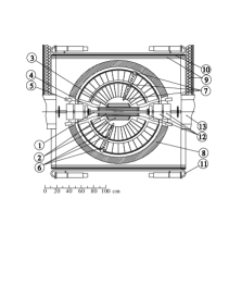
The SND detector [3, 4] (Fig. 1) consists of two cylindrical drift chambers for charge particle tracking, calorimeter, and a muon system.

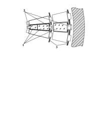
The main part of the detector is a three-layer spherical calorimeter, based on NaI(Tl) crystals. The pairs of counters of the two inner layers, with thickness of 2.9 and 4.8 $X_{0}$ respectively, where $X_{0}=2.6~{}\mathrm{cm}$ is a radiation length, are sealed in thin aluminum containers, fixed to an aluminum supporting hemisphere. Behind it, the third layer of NaI(Tl) crystals, 5.7 $X_{0}$ thick, is placed (Fig. 2). The total thickness of the calorimeter for particles, originating from the center of the detector, is equal to 34.7 cm (13.4 $X_{0}$). The total number of counters is 1632, the number of crystals per layer varies from 520 to 560. The angular dimensions of the most of crystals are $\Delta\phi=\Delta\theta=9^{\circ}$, the total solid angle is $90\%$ of $4\pi$.

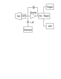
The electronics channel (Fig. 3) consists of:

1. phototriode with an average quantum efficiency of the photocathode for the NaI(Tl) emission spectrum of about $15\%$ and gain of about 10 [5]. The light collection efficiency varies from 7 to 15 $\%$ for different calorimeter layers,

2. charge sensitive preamplifier (CSA) with a conversion coefficient of  0.7 V/pC,

3. 12-channel shaping amplifier (SHA) with a remote controlled gain that can be set to any value in the range from 0 to a maximum with a resolution of 1/255.

4. 24-channel 12 bit analog to digital converter (ADC) with a maximum input signal $U_{\mathrm{max}}=2\mathrm{V}$,

5. in addition the SHA produces special signals for the first level trigger, the most important of which is the analog sum of all calorimeter channels — the total energy deposition.

Each calorimeter channel can be tested using a precision computer controlled calibration generator. The amplitude of its signal can be set to any value from 0 to 1 V with a resolution of 1/4096. The equivalent electronics noise of individual calorimeter counters lies within a range of 150-350 keV.

3 Algorithm of the detector calibration with cosmic muons

The calibration procedure is based on the comparison of experimental energy depositions in the calorimeter crystals for cosmic muons with Monte Carlo simulation. The simulation was carried out by means of the UNIMOD2 [6] code, developed for simulation of $e^{+}e^{-}$ colliding beam experiments. Simulated were muons crossing the sphere with a radius of 80 cm, centered at the beam crossing point, and containing all calorimeter crystals. The cosmic muon generation program is based on data from [7]. Experimental data on the energy and angular spectra of cosmic muons were approximated using the following formula:

$${\partial N\over\partial p\partial\theta}=F_{0}\cdot\cos^{k}\theta\cdot\exp\biggl{[}-{\ln^{2}(p/p_{0})\over 2\sigma^{2}}\biggr{]},$$ (1)

where $F_{0}=3\cdot 10^{-6}{\mathrm{cm}}^{-2}{\mathrm{s}}^{-1}{\mathrm{ster}}^{-1}{\mathrm{(MeV/c)}}^{-1}$ — the flux of muons with a momentum of $p=p_{0}=500\mathrm{MeV/c}$ at $\theta=0$, $\theta$ — angle between the muon momentum and vertical direction, $k=2.86$, $\sigma=(2.86-\cos\theta))/1.54$. The data from [7], on the relative abundances of positive and negative muons, were approximated using the following expression:

$$N_{+}/N_{-}=1,0+0,35\cdot\exp\biggl{[}-0,22\ln^{2}\biggl{(}{p\over 7\mathrm{GeV/c}}\biggr{)}\biggr{]}.$$ (2)

The passage of particles through the detector was simulated by means of the UNIMOD2 code. As a result the energy depositions in the calorimeter crystals were calculated in each event. A total of 1 000 000 cosmic events were simulated.

The simulated events were processed as follows. The track of cosmic muon was fitted to the hit crystals and expected track lengths in each crystal were calculated. Energy depositions $E_{\mathrm{i}}$ and track lengths $l_{\mathrm{i}}$ were summed over event sample for each crystal separately and for each crystal their ratio was calculated: $C_{\mathrm{mc}}(\mathrm{MeV/cm})=\langle E(\mathrm{MeV})\rangle/\langle l(\mathrm{cm})\rangle$. Brackets denote averaging over event samples. Then the calorimeter channels were calibrated electronically, using the generator. In order to account for the electronics nonlinearity, the calibration data were taken at two significantly different values of SHA gain and wide range of calibration generator amplitudes, covering the whole dynamic range of the ADCs. In addition, data were taken at a working value of the SHA gain.

Using all these data and assuming that the dependence of the ADC counts $S_{\mathrm{adc}}$ on the generator amplitude $U_{\mathrm{gen}}$ is described by a second order polynomial, and that the generator amplitude itself linearly depends on generator code, one can obtain $a,~{}b,~{}c,~{}p,~{}K_{\mathrm{u}}$ constants, defined by the following expressions:

$$S_{\mathrm{adc}}=aU_{\mathrm{gen}}^{2}+bU_{\mathrm{gen}}+c~{}~{}~{}\mathrm{and}~{}~{}~{}U_{\mathrm{gen}}=K_{\mathrm{u}}(G+p),$$ (3)

where $G$ and $p$ are a generator code and pedestal respectively, $K_{\mathrm{u}}$ - the relative SHA gain. The next step is to obtain from these intermediate results the final constants $A$, $B$, and $C$ for the working values of SHA gain, from the knowledge of which one can calculate the equivalent generator code $G$ for any measured ADC count:

$$G=AS_{\mathrm{adc}}^{2}+BS_{\mathrm{adc}}+C.$$ (4)

It relates an ADC count to a corresponding generator code, which allows the linearization of the ADC response.

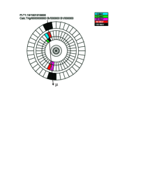
The next stage is processing of the experimental events. About 1.5 million events (Fig. 4) are needed to be collected in special data taking runs with total duration of 4.5 hours. The processing itself is the same as that of the simulated events, but now the initial ADC counts are first transformed into equivalent generator codes. As a result, values of $C_{\mathrm{exp}}(\mathrm{Gen/cm})=\langle G(\mathrm{Gen})\rangle/\langle l(\mathrm{cm})\rangle$ for each crystal are obtained. The meaning of $C_{\mathrm{exp}}$ is a code, which should be written into the generator to produce signals on CSA input, equivalent to an average input signal produced by a 1 cm long muon track.

Using $C_{\mathrm{exp}}(\mathrm{Gen/cm})$ and $C_{\mathrm{mc}}(\mathrm{MeV/cm})$, for each crystal we can calculate

$$C_{\mathrm{cal}}(\mathrm{MeV/Gen})=C_{\mathrm{mc}}(\mathrm{MeV/cm})/C_{\mathrm{exp}}(\mathrm{Gen/cm})~{}~{}~{}\mbox{---}$$ (5)

an equivalent generator code, corresponding to an energy deposition of 1 MeV in a crystal. Then the gains of the SHA channels are adjusted to equalize contributions of different crystals into the total energy deposition signal and the final generator calibration pass is carried out. It yields the coefficients $a_{\mathrm{k}}$, $b_{\mathrm{k}}$, and $c_{\mathrm{k}}$, needed to transform $S_{\mathrm{adc}}$ into MeV according to the following formula:

$$E(\mathrm{Mev})=a_{\mathrm{k}}S_{\mathrm{adc}}^{2}+b_{\mathrm{k}}S_{\mathrm{adc}}+c_{\mathrm{k}}.$$ (6)

The use of the precision generator as a reference calibration source is very convenient not only because its linearity is much higher than that of the ADC, but it also simplifies the replacement of any element of the electronics channel, except the CPA or generator itself. All what is needed after that is to recalibrate the calorimeter with the generator.

4 The description of the event processing algorithm

The goal of the experimental and simulated events processing is to obtain the normalized ratios $C_{\mathrm{mc}}(\mathrm{MeV/cm})$ and $C_{\mathrm{exp}}(\mathrm{Gen/cm})$. The need for normalization of the energy deposition to the unit track length in a crystal arises from the fact that the raw energy deposition spectra in crystals are very wide and have very weakly pronounced maxima. On the other hand, such a normalization reduces systematic errors due to possible differences in the angular distributions of simulated and real muons, and differences in the directions of crystals axes over the calorimeter. The simulated and experimental events are processed using the same computer code. The only difference is that before processing of a simulated event it is checked for passing the experimental trigger. The following selection criteria are used for event selection: the total number of hit crystals must be from 5 to 25. Crystals with energy depositions smaller than the threshold value (currently 5 MeV) are discarded. Similarly discarded are crystals with ADC counts less than 20. An event is selected if more than four hit crystals survive these cuts. For those crystals a straight line is fitted, using a least squares method, i. e. the sum of squares of distances from the crystal centers to the line is minimized. The line is parametrized as:

$$\vec{r}=\vec{R}+\vec{v}t,$$ (7)

where $\vec{R}$ is an arbitrary point on the line, $\vec{v}$ is a unitary vector in the direction of the line, $t$ — parameter. Then, the squared distance from the center of i-th crystal to the line is:

$$L_{\mathrm{i}}^{2}=(\vec{X_{\mathrm{i}}}-\vec{R})^{2}-(\vec{v}(\vec{X_{\mathrm{i}}}-\vec{R}))^{2},$$ (8)

where $\vec{X_{\mathrm{i}}}$ is a radius-vector of the crystal center. The minimized function is:

$$F_{\mathrm{min}}(\vec{R},\vec{v})=\sum\limits_{\mathrm{i}}L_{\mathrm{i}}^{2}/\sigma_{\mathrm{i}}^{2},$$ (9)

where $\sigma_{\mathrm{i}}$ is assumed to be equal to a half height of an i-th crystal. One point on a line can be determined immediately:

$$\vec{R_{0}}={\sum\limits_{\mathrm{i}}\vec{X_{\mathrm{i}}}/\sigma_{\mathrm{i}}\over\sum\limits_{\mathrm{i}}1/\sigma_{\mathrm{i}}^{2}}.$$ (10)

The direction of vector $\vec{v}$, is determined by a maximum of the quadratic form $F(\vec{R_{0}},\vec{v})$.

$$F(\vec{R_{0}},\vec{v})=\sum\limits_{\mathrm{i}}(\vec{v}(\vec{X_{\mathrm{i}}}-\vec{R_{0}}))^{2}/\sigma_{\mathrm{i}}^{2}.$$ (11)

In other words, $\vec{v}$ must have the same direction as an eigenvector of $A$, matrix of this quadratic form, corresponding to its maximal eigenvalue. Here

$$A_{\mathrm{mn}}=\sum\limits_{\mathrm{i}}((X_{\mathrm{i}}^{\mathrm{m}}-R_{0}^{\mathrm{m}})(X_{\mathrm{i}}^{\mathrm{n}}-R_{0}^{\mathrm{n}})/\sigma_{\mathrm{i}}^{2}),$$ (12)

$\mathrm{m,~{}n}=1,2,3$ — coordinate indices. The equation for $\vec{v}$ was solved using an iterative procedure:

$$\vec{v}_{\mathrm{n+1}}=A\vec{v}_{\mathrm{n}}/|A\vec{v}_{\mathrm{n}}|.$$ (13)

As seed value the unitary vector in the direction of the line between the centers of the two most distant crystals in the event is used. On each iteration step the presence of hit crystals at distances greater than $2\sigma_{\mathrm{i}}$ from the line is checked. If such crystals exist, two options are considered. The first one is to remove the most distant crystal from the list, the second one is to remove the crystal, most distant from the point $\vec{R_{0}}$. For both cases the fitting of the line is repeated and the final choice is based on the minimal value of $F_{\mathrm{min}}(\vec{R_{0}},\vec{v})$. If there are more than one crystal to be discarded then the event is rejected completely. From the remaining events only those are selected where $F_{\mathrm{min}}(\vec{R_{0}},\vec{v})$ divided by the number of hit crystals is less than 0.7 (Fig. 6).

After that, the expected lengths of the muon track $l_{\mathrm{ij}}$ in each crystal are calculated and averaged over the whole event sample together with the energy depositions $E_{\mathrm{ij}}$. The values of average track lengths $\langle l_{\mathrm{i}}\rangle$ and energy depositions $\langle E_{\mathrm{i}}\rangle$ are used then to calculate the energy deposition per unit track length $C_{\mathrm{i}}=\langle E_{\mathrm{i}}\rangle/\langle l_{\mathrm{i}}\rangle$. Here $i$ and $j$ are the crystal and the event numbers, respectively.

To estimate the statistical error in $C_{\mathrm{i}}$, the event sample is divided into groups of 50 events each and within each group the ratio $R_{i}=\langle E_{i}\rangle/\langle l_{i}\rangle$ is calculated. Then, the error $\sigma_{\mathrm{Ri}}$ in $C_{\mathrm{i}}$ can be estimated as $\sigma_{\mathrm{Ri}}=(\langle R_{\mathrm{i}}^{2}\rangle-\langle R_{\mathrm{i}}\rangle^{2})^{1/2}/\sqrt{N}$, where $N$ is a number of groups.

The total CPU time, required for processing of $1.5\cdot 10^{6}$ cosmic events is 2.5 hours on VAXstation 4000/60.

5 Events processing results. Comparison of experimental and simulated distributions

The mean $\langle C_{\mathrm{mc}}\rangle$ and their RMS values are shown in the Table 1. The necessity of normalization of energy depositions in crystals to a unitary track length was studied. To this end the events with muons going through drift chamber were processed, and the corresponding $C_{\mathrm{mc}}^{1}$ coefficients were calculated. The ratios of $\langle C_{\mathrm{mc}}/C_{\mathrm{mc}}^{1}\rangle$ and their RMS are also presented in the Table 1 together with the corresponding ratios of mean energy depositions $\langle E/E^{1}\rangle$. The data show, that the normalization significantly reduces the dependence of coefficients on the angular distribution of muons.

The distributions of experimental events over number of hit crystals with energy depositions higher than threshold value and over $F_{\mathrm{min}}(\vec{R_{0}},\vec{v})$ are in good agreement with the simulated ones (Fig. 5, 6). Small differences between experimental and simulated distributions may be attributed to inaccuracies in the angular and energy spectra of the primary particles and first level trigger simulation. This also may cause small differences in the distributions over the angle relative to vertical direction (Fig. 7). Shown in Fig. 8 are distributions over total energy deposition in the detector, normalized to a unitary track length also agree well.

A comparison of average track lengths of muons in the calorimeter crystals for the experimental and simulated events was carried out. The results are listed in Table 2. The statistical uncertainty of the $C_{\mathrm{exp}}$ coefficients is less than $1~{}\%$ for all three layers of the calorimeter. At the same time the uncertainties of the corresponding coefficients for simulated events are determined by simulation statistics.

6 Energy resolution of the calorimeter. Implementation of the calibration procedure

The energy resolution of the calorimeter was studied using $e^{+}e^{-}\rightarrow e^{+}e^{-}$ and $e^{+}e^{-}\rightarrow\gamma\gamma$ processes. The energy distributions for electrons are depicted in Fig. 9. The events with polar angles of the particles in the range $45\leq\theta\leq 135$ degrees and acollinearity angle less than 10 degrees were selected. To estimate the energy resolution quantitatively, the spectra in Fig. 9 were fitted by a function

$$F(E)=A\cdot\exp\biggl{\{}-{1\over 2}\cdot\biggl{[}\biggl{(}{\ln(\eta)\over t_{\mathrm{x}}}\biggr{)}^{2}+t_{\mathrm{x}}^{2}\biggr{]}\biggr{\}},$$ (14)

$$\eta=1+{t_{\mathrm{x}}(E-E_{\mathrm{m}})\over\sigma}\cdot{\sinh(t_{\mathrm{x}}\sqrt[]{\ln 4})\over t_{\mathrm{x}}\sqrt[]{\ln 4}},$$

where $E$ is a particle energy, $E_{\mathrm{m}}$ — the position of maximum, $A$ — normalization coefficient, $t_{\mathrm{x}}$ - the asymmetry parameter, $\sigma$ is a full width of the distribution at half maximum divided by 2.36. $A$, $E_{\mathrm{m}}$, $\sigma$, and $t_{\mathrm{x}}$ were treated as free parameters during fitting. Energy resolution was defined as $\sigma_{\mathrm{E}}/E=\sigma/E_{\mathrm{m}}$.

Experimental and Monte Carlo resolutions of the calorimeter at 500 MeV are respectively $3.7~{}\%$ and $5.5~{}\%$ for photons and $3.5~{}\%$ and $5.2~{}\%$ for electrons. Peak and mean values of the experimental and simulated distributions agree to a level of about $1~{}\%$, but the widths of experimental distributions are significantly larger. The possible explanation of the broadening of the experimental spectra could be electronics instability, systematic errors in calibration procedure and nonuniformity of light collection efficiency over the crystal volume.

Study of the electronics and photodetector stability showed, that it can attribute to a maximum of $1~{}\%$ shifts for the time duration of the collection of energy deposition spectra. Systematic biases were estimated by comparison of the calibration coefficients with those obtained using a special procedure based on minimization of the width of the energy deposition spectrum in the calorimeter for $e^{+}e^{-}$ events. Such a calibration was carried out using experimental statistics collected in 1996 [8]. The average bias of coefficients relatively to those obtained with cosmic calibration was $3~{}\%$ for the first layer. No statistically significant bias was found in other two layers. The RMS difference in calibration coefficients, obtained using cosmic and $e^{+}e^{-}$ calibration procedures is close to $3\div 5~{}\%$. The resulting energy resolution after $e^{+}e^{-}$ calibration was close to $5.0~{}\%$ for photons and $4.6~{}\%$ for electrons, which is still worse than that expected from Monte Carlo simulation.

A Monte Carlo simulation was carried out taking into account a nonuniformity of light collection efficiency over the crystal volume. The results are shown in Fig. 10 together with the experimental distribution. The energy resolution for simulated events decreased to $4.1~{}\%$. It shows that the broadening of experimental spectra was mainly determined by the nonuniformity of light collection efficiency over the crystal volume.

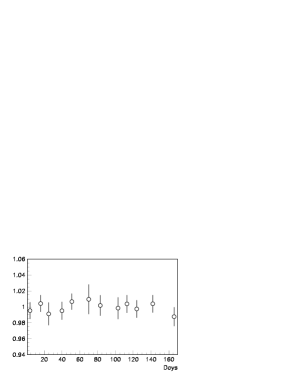
The cosmic calibration procedure was used during a five month experiment with SND at VEPP-2M in 1996 [8]. Relative shifts in calibration coefficients are shown in Fig. 11. It can be seen, that for a one week period between consecutive calibrations, the mean shift of the coefficients is less than $2~{}\%$ and RMS of their random spread is $1\div 2~{}\%$.

7 Conclusion

With the help of the described procedure of SND calorimeter calibration a statistical accuracy of $1~{}\%$ in calibration coefficients and energy resolution of $5.5~{}\%$ for 500 MeV electromagnetic showers was achieved. Mean energy depositions agree with simulation at a level better than $1~{}\%$. The total time, required for calorimeter calibration is not more than 5 hours.

Table 1: $C_{\mathrm{mc}}$ coefficients. Comparison of calibration results based on different muon samples (MC).

Layer number	$C_{\mathrm{mc}}$	$\sigma_{\mathrm{C}}(\mathrm{MeV/cm})$	$\langle C_{\mathrm{mc}}/C_{\mathrm{mc}}^{1}\rangle$	$\sigma$	$\langle E/E^{1}\rangle$	$\sigma$
I	5.38	0.14	0.99	0.02	0.83	0.04
II	5.43	0.09	0.96	0.03	0.71	0.05
III	5.61	0.08	0.99	0.03	0.68	0.05

Table 2: Comparison of mean track lengths of muons in calorimeter crystals for the experimental and simulated events. The statistical uncertainty of $C_{\mathrm{mc}}$.

Layer number	$\langle\langle l_{\mathrm{mc}}\rangle/\langle l_{\mathrm{exp}}\rangle\rangle$	$\sigma$	$\sigma_{\mathrm{Ri}}/\sqrt[]{N}$
I	1.01	0.02	$1.4\%$
II	1.00	0.01	$1.0\%$
III	1.00	0.01	$0.9\%$

Figure 1: SND detector, section along the beams; 1 — beam pipe, 2 — drift chambers, 3 — scintillation counters, 4 — light guides, 5 — PMTs, 6 — NaI(Tl) crystals, 7 — vacuum phototriodes, 8 — iron absorber, 9 — streamer tubes, 10 — 1cm iron plates, 11 — scintillation counters, 12 and 13 — elements of collider magnetic system.

Figure 2: NaI(Tl) crystals layout inside the calorimeter: 1 — NaI(Tl) crystals, 2 — vacuum phototriodes, 3 — aluminum supporting hemispheres.

Figure 3: Electronics channel of the SND calorimeter: NaI — NaI(Tl) scintillator, VPT — vacuum phototriode, Preamp — charge sensitive preamplifier, Att — computer controlled attenuator, Shaper — shaping amplifier, Generator — calibration generator, ADC — analog to digital converter, Trigger — first level trigger.

Figure 4: Example of cosmics event selected by calibration procedure.

Figure 5: Distributions over number of hit crystals for the events with energy depositions above certain threshold. N — number of hit crystals. Circles — experimental events, histogram — MC simulation.

Figure 6: Distribution over residual values of minimized function in experimental and simulated events.

Figure 7: Distribution over the track angle with respect to a vertical direction.

Figure 8: Total energy depositions in the calorimeter per unit track length in experimental and simulated events.

Figure 9: Energy spectra for 500 MeV electrons. $E$ is a measured energy, $E_{0}$ is the beam energy.

Figure 10: Energy spectra for 500 MeV electrons. The nonuniformity of light collection efficiency over the crystal volume was taken into account in Monte Carlo simulation. $E$ is the electron measured energy, $E_{0}$ is the beam energy.

Figure 11: The calibration coefficients spread. Points — average ratio of the current calibration results to the preceding ones, error bars — FWHM of the distributions of these ratios over the whole calorimeter layer divided by 2.36. Horizontal axis shows the number of days elapsed from the first calibration. Shown are the results for the second layer. Other calorimeter layers behave similarly.

References

- [1] M.N.Achasov et al., in Proceedings of Workshop of the Sixth International Conference on Instrumentation for Experiments at e+e- Colliders, Novosibirsk, Russia, February 29 - March 6, 1996, Nucl Instr and Meth., A379(1996),p.505.
- [2] J.A.Bakken et al., Nucl. Instr. and Meth., A275(1989), p.81.
- [3] V.M.Aulchenko et al., in Proceedings of Workshop on Physics and Detectors for DANE,Frascati, April 1991 p.605.
- [4] V.M.Aulchenko et al., The 6th International Conference on Hadron Spectroscopy, Manchester, UK, 10th-14th July 1995, p.295.
- [5] P.M.Beschastnov et al., Nucl Instr and Meth., A342(1994), p.477.
- [6] A.D.Bukin, et al., in Proceedings of Workshop on Detector and Event Simulation in High Energy Physics, The Netherlands, Amsterdam, 8-12 April 1991, NIKHEF, p.79.
- [7] Muons, A.O.Vajsenberg, Amsterdam:North-Holland, 1967.
- [8] M.N.Achasov et al., Status of the experiments with SND detector at collider VEPP-2M in Novosibirsk, Novosibirsk, Budker INP 96-47, 1996.