OPTICAL MICROSPHERE RESONATORS: OPTIMAL COUPLING TO HIGH-Q WHISPERING-GALLERY MODES
Abstract
A general model is presented for coupling of high- whispering-gallery modes in optical microsphere resonators with coupler devices possessing discrete and continuous spectrum of propagating modes. By contrast to conventional high-Q optical cavities, in microspheres independence of high intrinsic quality-factor and controllable parameters of coupling via evanescent field offer variety of regimes earlier available in RF devices. The theory is applied to the earlier-reported data on different types of couplers to microsphere resonators and complemented by experimental demonstration of enhanced coupling efficiency (about 80%) and variable loading regimes with fused silica microspheres.
I INTRODUCTION
High- optical microsphere resonators currently attract growing interest in experimental cavity QED [1, 2, 3], measurement science, [4, 5] frequency stabilization and other photonics applications [6, 7]. Stemming from extensive studies of Mie resonances in microdroplets of aerosols [8](observed via elastic and inelastic scattering of free-space beams), further studies of laboratory-fabricated solid-state microspheres focus on the properties and applications of highly-confined whispering-gallery (WG) modes. The modes of this type possess negligible electrodynamically-defined radiative losses (the corresponding radiative quality factors and higher), and are not accessible by free-space beams and therefore require employment of near-field coupler devices. By present moment, in addition to the well known prism coupler with frustrated total internal reflection [9, 10], demonstrated coupler devices include sidepolished fiber coupler [5, 11, 12] and fiber taper [13]. The principle of all these devices is based on providing efficient energy transfer to the resonant circular total-internal-reflection-guided wave in the resonator (representing WG mode) through the evanescent field of a guided wave or a TIR spot in the coupler.
It is evident a priori that efficient coupling maybe expected upon fulfillment of two main conditions: 1)phase synchronism and 2)significant overlap of the two waves modelling the WG mode and coupler mode respectively. Although reasonable coupling efficiency has been demonstrated with three types of devices (up to few tens of percents of input beam energy absorbed in a mode upon resonance), no systematic theoretical approach has been developed to quantify the performance of coupler devices. It still remained unclear whether it is possible at all and what are conditions to provide complete exchange of energy between a propagating mode in a coupler device and the given whispering gallery mode in high- microsphere. Answers to these questions are of critical importance for photonics applications and also for the proposed cavity QED experiments with microspheres.
In this paper, we present a general approach to describe the near-field coupling of high- whispering-gallery mode to a propagating mode in dielectric prism, slab or waveguide structure. Theoretical results present a complete description and give a recipe to obtain optimal coupling with existing devices. We emphasize the importance of the introduced loading quality-factor parameter and its relation with the intrinsic -factor of WG modes as crucial condition to obtain optimal coupling. Theoretical consideration is complemented by experimental tests of variable loading regimes and demonstration of improved coupling efficiency with prism coupler.
II GENERAL CONSIDERATIONS
Let us examine excitation of a single high- whispering gallery mode with high quality-factor by () travelling modes in an evanescent wave coupler. This coupler can either have infinite number of spatial modes (, as in prism coupler [9, 10] and slab) or only one mode (, as in tapered fiber[13] and integrated channel waveguide).
We shall start with simple description of the system using lumped parameters and quasigeometrical approximation.
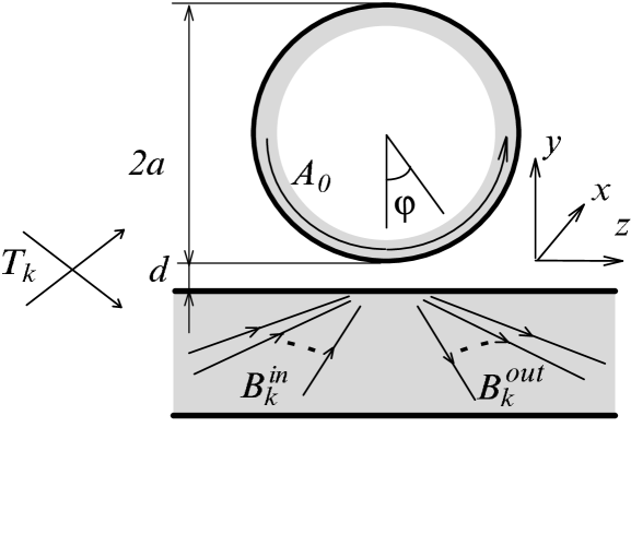
Let be the amplitude of a circulating mode of total internal reflection in the resonator (see Fig.1) to model the whispering-gallery mode. Let the pump power be distributed in the coupler between its modes so that is the amplitude of mode () and is the slow varying amplitude with equal to total pump power. Let us assume for simplicity that coupling between different modes is absent without the resonator.
Assuming that the coupling zone is much smaller than the diameter of the resonator, we can introduce local real amplitude coefficients of transmittance to describe the coupling of the resonator with all modes of the coupler (either guided or leakage ones) and the internal reflectivity coefficient . We shall denote arrays of transmittance coefficients and amplitudes as vectors and respectively. If the quality-factor of the resonator mode is high enough, then a single circle gives only small contribution to the mode buildup and therefore . In this case (neglecting for simplicity absorption and scattering losses in the coupler ) we obtain
| (1) |
The equation for the mode of the resonator will be the following:
| (2) | |||||
| (3) |
where is the circulation time for the mode travelling inside the sphere, is approximately equal to the circumference of the sphere, is the wavelength, is the refraction index, is the speed of light and is the linear attenuation in the resonator caused by scattering, absorption and radiation.
In the above representation the microsphere is equivalent to a ring resonator formed by mirrors with transmittances and filled with lossy medium, or, in case of single-mode coupling, as pointed in [11], to a Fabry-Perot resonator of the length with totally reflecting rear mirror.
If propagation losses are small, then near the resonance frequency , , where is integer, by expanding from (3) we obtain:
| (4) |
where
| (5) |
We introduce here another important coefficient:
| (6) |
This coefficient describes mode matching and shows how close the field in the couplers matches the near field of resonator mode.
The term originates from intrinsic quality factor while describes loading i.e. mode energy escape to all modes of the coupler. Hereafter we shall mark all values associated with coupler by index ‘’ and values associated with microsphere by index ‘’.
Equation (4) is a classical equation for the amplitude of the resonator pumped by harmonical field.
As will be shown below, coefficients can be calculated as normalized overlap integrals of the fields of the microsphere mode and modes of the coupler. The difference from Fabry-Perot resonator is that for the microsphere, coefficients are not fixed parameters but instead, strongly depend on geometry of coupling (e.g. exponentially on the value of the gap between microsphere and coupler) and are therefore in hands of experimentalist. As we already emphasized in [9], it is the controllable relation between and that defines coupling efficiency upon given configuration (accounting both for mode overlap and synchronism and optimized loading to provide energy exchange between resonator and coupler). Stationary solution for (4) has the typical form:
| (7) |
Field amplitude in the resonator will be maximal at (intrinsic quality-factor equals the loaded ). The output stationary amplitudes are
| (8) |
and total output intensity in this case has lorentzian shape:
| (9) |
It can be easily seen from this equation that the output signal can be considered as the result of interference of the input and the ”re-emission” from the resonator. Note that mode distribution of the second term in (8) (resonator mode emission pattern) does not depend on the input distribution.
The most important case of (8) is the regime of ideal matching (), obtained with when the fraction of the input power fed into the resonator mode is maximal. (Single-mode coupler is always ”mode-matched”.) In this case, provided , output intensity turns to zero i.e. the entire input power is lost inside the resonator. This regime is usually called critical coupling. Sometimes coupling is characterized by the fractional depth of the resonance dip in intensity transmittance observed upon varying the frequency of exciting wave in the coupler; from (9) can be expressed as follows
| (10) | |||
| (11) |
In case of critical coupling (100%). In case of nonideal matching, critical coupling may be observed until (partial matching) if the output is mode-filtered to pick up only part of the coupler modes. In this case leakage into other modes may be considered as additional internal losses, and critical coupling is obtained with lower loaded quality factor when . If (overcoupling) then for matched coupling the output wave in resonance has the sign opposite to that out of resonance i.e. the resonator shifts phase by . It is appropriate to note here that in traditional high-Q optical resonators comprised of mirrors, the quality-factor is limited by the mirrors’ finesse i.e. by loading. With microspheres, the situation is opposite, and the primary role belongs to the intrinsic quality-factor.
III DIRECTIONAL COUPLER APPROACH
The goal of this section is to determine parameters of the coupler-resonator system from the electrodynamical point of view. In the recent paper [15] by D.R.Rowland and J.D.Love, famous for their popular book on the theory of optical waveguides [16], the problem of coupling with whispering-gallery modes is addressed on the basis of the model of distributed coupling between a travelling surface mode in cylindrical resonator and a given mode in a planar (slab) waveguide. In this approach, the coupling problem leads to the necessity to solve a system of differential equations, which in our designations looks as follows:
| (12) | |||||
| (13) |
Coefficients and (describing perturbation of wave numbers and of modes of the resonator and the coupler) and distributed coupling coefficients can be calculated explicitly as field cross-section integrals (see [15] and references therein).
| (14) | |||
| (15) |
Here and are equivalent waveguide modes of the resonator and of the coupler respectively, normalized vs. power; the integration is done over cross-sections. Indexes and denote that the integration is done inside the microsphere and coupler respectively. In principle, conservation of energy requires that the two integrals in expression for be equal and this is frequently postulated. However, in common approximation that we also use here the above equality is secured only for phase-matched or identical waveguides, while in the opposite case the dependence of the two integrals on the gap is different. Nevertheless, to provide efficient coupling, this equality must be satisfied.
Parameters (15) are nonzero only in the coupling zone. It may seem that the coupler transmission matrix (CTM) and, subsequently, the above introduced lumped coefficients can be found from equations (13). However, analytical derivation of the output field amplitudes cannot be found from (13) with exception of few simple cases. It was perhaps due to this fact that the authors of [15] presented only numerical solution for their particular case. Moreover, in general case CTM is a complex 2x2 matrix and cannot be characterized by one real parameter.
Fortunately, the situation is more favorable for optical microsphere resonators with high loaded quality-factor , when . Indeed, from (5) it follows that . In a fused silica resonator with the diameter () and heavily loaded (intrinsic - factor can be of the order of in this case) . In practice is usually of the order of . It means that the field amplitude changes insignificantly over the coupling zone and can therefore be assumed constant in the second equation of (13), and the stationary amplitude . Therefore an approximate solution can be obtained:
| (16) | |||||
| (17) |
where
| (18) |
Equations (17) are practically identical to (3) if is closed into a ring. In the second equation of (17) we neglected small second-order terms while, however, keeping them in the first equation as they describe the coupler-induced shift in resonant frequency and the reduction of by loading.
| (19) | |||
| (20) |
IV VARIATIONAL APPROACH
Directional coupler approach can be easily generalized for multimode coupler. However expressions for the coupling parameters better suited for couplers with dense mode spectrum can be found in a more rigorous way directly from Maxwell equations using variational methods. Electric field in the resonator perturbed by coupler may be written in the form:
| (21) |
where are orthonormalized eigenmodes of the unperturbed lossless resonator without coupler
| (22) |
( is Kronecker symbol here). Rigorously speaking this normalization meets some difficulties for open dielectric resonators with finite radiative quality-factor [17]. In our consideration, however, we can avoid them by assuming eigenfrequences of interest to be purely real. For this we neglect the imaginary part that describes radiation losses and choose as the integration volume the sphere with a diameter much less than . Amplitudes are slowly varying and differ from circulating amplitude introduced before only in terms of normalization. One can easily see that
| (23) |
The equation for the field in the coupled sphere will have the form:
| (24) |
where the second term in brackets is additional polarization due to presence of the coupler, the third one describes damping associated with intrinsic losses in the resonator, and the right part is the polarization caused by the pump wave. Dielectric susceptibilities are equal to inside and unity outside the spherical resonator and the coupler correspondingly. Substituting (21) into (24) and multiplying this equation by , after integration over the entire volume and omitting small terms we obtain:
| (25) |
where and
| (26) |
is the new resonance frequency shifted due to the coupler, in total agreement with (20). Let us express the field in the coupler as expansion in travelling modes in direction:
| (27) |
Guided localized modes of the coupler in this description can also be easily taken into account if we choose as
| (28) |
The coupler modes are normalized in such a way that
| (29) |
(here is delta-function and is the magnetic field corresponding to the mode). Integration is performed over the cross-section orthogonal to -axis. Amplitudes (slowly varying with and ) describe distribution of the pump wave in coupler modes. Substituting (27) into the wave equation:
| (30) |
we obtain
| (31) |
The second term in brackets (30) determines the change of the wavenumber (phase velocity) for the given mode in the coupling zone. Taking vector product of this equation with and integrating over the cross-section, we obtain formal solutions for slowly varying amplitudes:
| (32) | |||||
| (33) |
Substituting (27) into (25) using (33) and omitting , we finally obtain the following equation for the amplitude of the mode in the resonator:
| (34) |
and
| (35) | |||||
| (36) |
in natural agreement with (20). Total agreement with (4-8) becomes apparent if we put
| (37) |
For high- WG modes , and as the field drops outside the resonator approximately as (), the dependence of on can be approximated as follows: . If the coupler is straight in direction (as in most demonstrated couplers to date), we obtain:
| (38) |
V APPLICATION TO DEMONSTRATED COUPLERS
Let us now use the developed approach for the analysis of coupling of whispering-gallery modes with optical fiber. As soon as according to (refkcoupl), possibility of efficient coupling critically depends on the value of the loading quality-factor and its relation with the intrinsic , in this section we shall focus on calculation of and discuss briefly methods to achieve phase synchronism and mode matching with different couplers.
To date, two types of optical fiber coupler to WG modes in microsphere were demonstrated. The first one is the eroded fiber coupler [5, 11, 12], where evanescent field of a propagating waveguide mode becomes accessible due to partial removal of the cladding in a bent section of the fiber. The recently demonstrated second type of the fiber coupler is based on the stretched section of a single mode fiber employing the mode conversion of the initial guided wave into waveguide modes of cladding tapered to the diameter of few microns [13].
The most interesting type of strong confinement modes of the sphere - with radius (where radial index is small) and the mode in the fiber of radius can be approximated as follows [18, 16]:
| (41) | |||||
| (44) |
where
| (45) | |||||
| (46) |
Using (20) and several approximations, we can now calculate
| (47) |
where is the gap between the resonator and the fiber and . To obtain optimal coupling, one has to require matching the propagation constants in the argument of the second exponent of (47) () as in [13]. In this case, using approximations for eigenfrequences in the resonator, one can obtain optimal radius of the fiber and the loaded .
| (48) | |||
| (49) |
Using the above expressions, we can try to compare our calculations with the experimental data reported in [13] for , and . The measured was with . Using (11) we can obtain and . Calculations with (49) give – in agreement with the experiment.
It is appropriate to note here that in principle, as follows from (47), the minimum of does not correspond to phasematching () and is shifted to smaller . This minimum is also not very sharp ( - several percents of ). However this case deserves special consideration, because for smaller the approximations we use here will give larger (more than 10%) error. It is also important that the loaded increases very quickly with the size of the resonator (as ), and in this way the range of possible applications of such coupler becomes restricted. Even for very small fused-silica spheres, optimal radius of most common silica fiber does not correspond to single-mode operation implying further technical complications in using this type of coupler.
The conclusions of our theory also correlate with the data on limited efficiency of sidepolished optical fiber couplers [5, 11, 12]. Indeed, with the typical monomode fibers having core index equal or smaller than that of the spheres (made from polystyrene or silica correspondingly in [5, 11, 12], with small microspheres one cannot satisfy phasematching because of relatively large diameter of standard cores, and with larger spheres coupling coefficient is too small (coupling -factor too high) to provide efficient power insertion into the resonator.
Efficient coupling (tens of %) with high-Q microspheres has been demonstrated with the planar (slab) waveguides [19]. This type of the coupler provides additional freedom compared to fiber waveguides because it allows free manipulation of the two-dimensional optical beams. Optimal width for mode is . In the meantime requirement of phase matching for efficient coupling implies optimization of the slab waveguide thickness . Using the same approach as above, we obtain:
| (50) |
It is appropriate to note here that either fibers or planar waveguides can also effectively excite modes with if the wavevector is inclined to the “equator” plane of the sphere (symmetry plane of the residual ellipticity) by angle . This conclusion becomes evident if we remember that the mode with is equivalent to a precessing inclined fundamental mode [10].
Prism coupler has been analyzed in our previous papers [9, 10] together with precession approach to the description of WG modes and theoretical and experimental investigation of the far field patterns. By contrast to waveguide couplers, where practical realization of high efficiency implies either precise engineering of the waveguide parameters, or the step-by-step search of the optimal contact point to the fiber taper, prism coupler allows systematic procedure of coupling optimization by manipulating the external beams. The two steps to achieve efficient coupling are 1)adjustment of the incidence angle of the input Gaussian beam inside the coupler prism and 2) adjustment of the angular size of the beam and to provide mode matching with far field of the WG mode in the prism ( factor).
| (51) |
The loading with the prism coupler is as follows:
| (52) |
Fig.2 summarizes the calculations of the loading quality-factor for different types of couplers (with optimized parameters) in form of the plots of under zero gap . The results in Fig.2 allow to quickly evaluate possibility to achieve critical coupling with the given size and intrinsic Q of the sphere, along the lines summarized in Sec.2 (11).
In our experiments employing high- WG microsphere resonators, we used prism coupler in most cases and believe that it remains the most flexible device as it provides ability of fine adjustment of both phase synchronism and mode matching via convenient manipulation of the apertures and incidence angles of free beams. Also, as seen in Fig.2, it provides a significant margin to obtain critical coupling with the spheres of various size and intrinsic Q. As a result, we routinely obtained coupling efficiencies to silica microspheres about with standard right-angle BK7 glass prisms limited by restricted mode overlap due to input refraction distortions of the symmetrical Gaussian beams. Use of cylindrical optics or higher refraction prisms to eliminate the mode mismatch () can significantly improve coupling efficiency and approach full exchange of energy under critical regime. (About coupling efficiency is demonstrated further in the experimental Sec.7).
To conclude this section, let us also note here that the critical coupling (that is characterized by maximal absorption of the input power in the resonator) is in fact useless for such applications as cavity QED or quantum-nondemolition experiments, because no recirculated power escapes the cavity mode. To be able to utilize the recirculated light, one has to provide the inequality (strong overcoupling). In other words, the intrinsic quality-factor has to be high enough to provide reserve for sufficient loading by the optimal coupler.
VI PRISM COUPLER: EXPERIMENTAL EFFICIENCY AND VARIABLE LOADING REGIMES
In order to illustrate the results of our analysis, we performed measurements to characterize coupling efficiency of the prism coupler with high-Q fused silica microspheres. As in our previous experiments, we used microspheres fabricated of high-purity silica preforms by fusion in a hydrogen-oxygen microburner (see description of the technique in [20]). The focus of present experiment was to obtain enhanced coupling by maximizing the mode matching
| (53) |
along with the lines briefly described in Sec.2. In our experiment, to diminish astigmatic distortions of the input gaussian beam at the entrance face of the coupler prism, we used equilateral prism of flint glass (SF-18, refraction index n= 1.72). As usual, the input beam (a symmetrical gaussian beam from a single-mode piezo-tunable He-Ne laser) was focused onto the inner surface of the prism, at the proximity point with the microsphere. The angle of incidence and the cross-section of the input beam were then optimized to obtain maximum response of a chosen WG mode. Initial alignment was done on the basis of direct observation of resonance interference in the far field, with the frequency of the laser slowly swept across the resonance frequency of the mode. With the given choice of prism material, optimal angle of incidence for excitation of whispering-gallery modes (close to critical angle of total internal refraction at the silica-glass interface) was approximately equal to 60 degrees so that astigmatic distortions of the input beam at the entrance face of the prism were minimized.
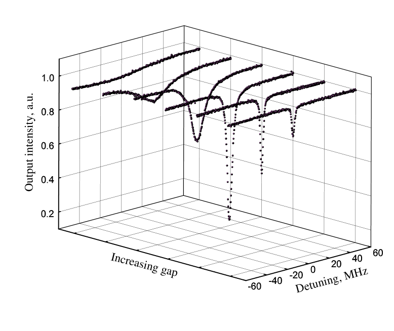
After preliminary alignment, the coupling efficiency was further maximized on the basis of direct observation of the resonance absorption dip: full intensity of the beam after the coupler prism was registered by linear photodetector and monitored on digital oscilloscope. Results obtained with a mode (possessing strongest confinement of the field in meridional direction) are presented in Fig.3 in form of the resonance curves observed upon successively decreasing coupling (stepwise increasing gap). Fig.3 illustrates good agreement of theory with experiment: indeed, resonance transmission decreases with loading until the quality-factor becomes twice smaller than the intrinsic ; after that, intensity contrast of the resonance decreases. Fig.4 presents explicitly the plot of the fitted experimental intensity dip versus the loaded quality-factor , which yields satisfactory agreement with parabolic prediction from the generalized expression (11). Maximal contrast of the resonance obtained in our experiment was (the ”deepest” curve in Fig.3).
VII CONCLUSION
We have presented a general approach to describe the near-field coupling of high- whispering-gallery modes in optical microsphere resonators to guided or free-space travelling waves in coupler devices with continuous and discrete spectrum of propagating modes.
A convenient formalism of the loaded quality-factor to describe the energy exchange between coupler modes and the resonator provides a quick algorithm to determine the efficiency of the given type of the coupler, under given value of the intrinsic quality-factor of WG modes.
Variable relation between the intrinsic -factor and loading losses (described by ) through energy escape to coupler modes is a distinctive new property of whispering-gallery resonators compared to conventional Fabry-Perot cavities: the latter are characterized by fixed coupling through the reflectivities of comprising low-loss mirrors. This unique ability to control the and coupling via WG mode evanescent field allows to obtain new regimes in the devices, analogous to those available in lumped-element RF and microwave engineering.
Theoretical estimates on the basis of the suggested theory are in good agreement with the reported data on the efficiency of different coupler devices including tapered, sidepolished fiber and slab waveguide.
Original experimental results include direct demonstration of variable loading and enhanced efficiency (up to about ) in prism coupler. Ease of control of phase synchronism and mode overlap between coupler and microsphere mode by adjusting the input beam parameters make the prism coupler versatile and efficient for various applications of high-Q microsphere resonators.
In conclusion, let us note that the near-field coupling may be not a unique method to efficiently excite highly confined whispering-gallery modes in microspheres. Simple estimates show that for example, recent advances in optical fiber grating fabrication methods [21] may allow to ”imprint” a Bragg-type critical coupler for high-Q WG modes directly on a sphere made of low-loss germanosilicate glass. This configuration might be of special interest for atomic cavity-QED experiments, where presence of bulky external couplers may destroy the field symmetry, complicate laser cooling of atoms etc.
ACKNOWLEDGMENTS
This research was supported in part by the Russian Foundation for Fundamental Research grant 96-15-96780.
REFERENCES
- [1] V.B.Braginsky, M.L.Gorodetsky, V.S.Ilchenko, ”Quality-factor and nonlinear properties of optical whispering-gallery modes”, Phys.Lett. A137, pp.393-6, 1989.
- [2] H.Mabuchi, H.J.Kimble, ”Atom galleries for whispering atoms: binding atoms in stable orbits around a dielectric cavity” Opt.Lett., 19, pp.749-751, 1994.
- [3] V.Sandoghdar, F.Treussart, J.Hare, V.Lefèvre-Seguin, J.-M.Raimond, S.Haroche, ”A very low threshold whispering gallery mode microsphere laser”, Phys.Rev. B54, pp.R1777-R1780, 1996.
- [4] S.Schiller, and R.L.Byer, ”High-resolution spectroscopy of whispering gallery modes in large dielectric spheres”, Opt.Lett.,16, pp.1138-1140, 1991.
- [5] A.Serpengüzel, S.Arnold, G.Griffel, ”Excitation of resonances of microspheres on an optical fiber”, Opt.Lett., 20, pp.654-656, 1994.
- [6] V.V.Vasiliev, V.L.Velichansky, M.L.Gorodetsky, V.S.Ilchenko, L.Hollberg, A.V.Yarovitsky, Quantum Electronics, High-coherence diode laser with optical feedback via a microcavity with ’whispering gallery’ modes”, Quantum Electronics,26,pp. 657-8 (1996)
- [7] L.Collot, V.Lefèvre-Seguin, M.Brune, J.-M.Raimond, S.Haroche, ”Very high- whispering gallery modes resonances observed on fused silica microspheres”, Europhys.Lett. 23(5), 327-333, 1993.
- [8] P.W.Barber, R.K.Chang, Optical effects associated with small particles, World Scientific, Singapore, 1988.
- [9] S.P.Vyatchanin, M.L.Gorodetsky, and V.S.Ilchenko, ”Tunable narrowband optical filters with whispering gallery modes” Zh.Prikl.Spektrosk.,56, pp.274-280, 1992 (in Russian).
- [10] M.L.Gorodetsky, V.S.Ilchenko, ”High-Q optical whispering gallery microresonators: precession approach for spherical mode analysis and emission patterns”, Opt.Comm., 113, 133-143, 1994.
- [11] G.Griffel, S.Arnold, D.Taskent, A.Serpengüzel, J.Connoly, and N.Morris, ”Morphology-dependent resonances of a microsphere-optical fiber system”, Opt.Lett.,21, pp.695-697, 1995.
-
[12]
N.Dubreuil, J.C.Knight, D.Leventhal, V.Sandoghdar, J.Hare, and V.Lefévre-Seguin,
J.M.Raimond, and S.Haroche, ”Eroded monomode optical fiber for whispering-gallery mode excitation in fused-silica microspheres”, Opt.Lett. 20, 1515, 1995. - [13] J.C.Knight, G.Cheung, F.Jacques and T.A.Birks, ”Phase-Matched excitation of whispering gallery mode resonances using a fiber taper” Opt.Lett., 22, pp.1129-1131,1997.
- [14] M.L.Gorodetsky, A.A.Savchenkov, V.S.Ilchenko, ”On the ultimate Q of optical microsphere resonators” Opt.Lett.,21, 453-455, 1996.
- [15] D.R.Rowland, J.D.Love, ”Evanescent wave coupling of whispering gallery modes of a dielectric cyllinder”,IEE Proc. J. 140, pp.177-188, 1993.
- [16] A.W.Snyder, J.D.Love, Optical waveguide theory, Chapman and Hall, London, 1983.
- [17] H.M.Lai, P.T.Leung, K.Young, P.W.Barber, and S.C.Hill, ”Time-independent perturbation for leaking electromagnetic modes in open systems with application to resonances in microdroplets”, Phys. Rev. A, 41, pp.5187-5198, 1990.
- [18] S.Shiller, ”Asymptotic expansion of morphological resonance frequencies in Mie scattering”, Appl.Opt.,32, pp.2181-2185, 1993.
- [19] N.Dubreuil, 1997 (private communication).
- [20] M.L.Gorodetsky and V.S.Ilchenko, ”Thermal nonlinear effects in optical whispering-gallery microresonators”, Laser Physics, 2, pp.1004-1009, 1992.
- [21] D.S.Starodubov, V.Grubsky, J.Feinberg, B.Kobrin, S.Juma, ”Bragg grating fabrication in germanosilicate fibers by use of near-UV light: a new pathway for refractive index changes”,Opt. Lett., 22, pp.1086-1088, 1997.