Statistical Mechanics in a Nutshell

1 Some Probability Theory

1.1 Constrained distributions

A random experiment has $n$ possible results at each trial; so in $N$ trials there are $n^{N}$ conceivable outcomes. (We use the word “result” for a single trial, while “outcome” refers to the experiment as a whole; thus one outcome consists of an enumeration of $N$ results, including their order. For instance, ten tosses of a die ($n=6,N=10$) might have the outcome “1326642335.”) Each outcome yields a set of sample numbers $\{N_{i}\}$ and relative frequencies $\{f_{i}=N_{i}/N,i=1\ldots n\}$. In many situations the outcome of a random experiment is not known completely: One does not know the order in which the individual results occurred, and often one does not even know all $n$ relative frequencies $\{f_{i}\}$ but only a smaller number $m$ ($m<n$) of linearly independent constraints

$$\sum_{i=1}^{n}G^{i}_{a}f_{i}=g_{a}\quad,\quad a=1\ldots m\,.$$ (1)

As a simple example consider a loaded die. Observations on this badly balanced die have shown that $6$ occurs twice as often as $1$; nothing peculiar was observed for the other faces. Given this information only and nothing else, i.e., not making use of any additional information that we might get from inspection of the die or from past experience with dice in general, all we know is a single constraint of the form (1) with

$$G_{1}^{i}=\left\{\begin{array}[]{rl}2:&i=1\\ 0:&i=2\ldots 5\\ -1:&i=6\end{array}\right.$$ (2)

and $g_{1}=0$.

The available data –in the form of linear constraints– are generally not sufficient to reconstruct unambiguously the relative frequencies $\{f_{i}\}$. These frequencies may be regarded as Cartesian coordinates of a point in an $n$-dimensional vector space. The $m$ linear constraints, together with $f_{i}\in[0,1]$ and the normalization condition $\sum f_{i}=1$, then just restrict the allowed points to some portion of an $(n-m-1)$-dimensional hyperplane.

1.2 Concentration theorem

Given an a priori probability distribution $\{p_{i}\}$ for the results $i=1\ldots n$, the probability that $N$ trials will yield the –generally different– relative frequencies $\{f_{i}\}$ is

$$\mbox{prob}(\{f_{i}\}|\{p_{i}\},N)={N!\over N_{1}!\ldots N_{n}!}\,p_{1}^{N_{1}}\ldots p_{n}^{N_{n}}\quad.$$ (3)

Here the second factor is the probability for one specific outcome with sample numbers $\{N_{i}\}$, and the first factor counts the number of all outcomes that give rise to the same set of sample numbers. With the definition

$${I}_{p}(f):=-\sum_{i}f_{i}\ln{f_{i}\over p_{i}}$$ (4)

and the shorthand notations $f=\{f_{i}\}$, $p=\{p_{i}\}$ we can also write

$$\mbox{prob}(f|p,N)=\mbox{prob}(f|f,N)\exp[N{I}_{p}(f)]\quad.$$ (5)

In particular, for two different data sets $\{f_{i}\}$ and $\{f^{\prime}_{i}\}$ the ratio of their respective probabilities is given by

$${\mbox{prob}(f|p,N)\over\mbox{prob}(f^{\prime}|p,N)}={\mbox{prob}(f|f,N)\over\mbox{prob}(f^{\prime}|f^{\prime},N)}\,\exp[N({I}_{p}(f)-{I}_{p}(f^{\prime}))]$$ (6)

where, by virtue of Stirling’s formula

$$x!\approx\sqrt{2\pi x}\,x^{x}e^{-x}\quad,$$ (7)

it is asymptotically

$${\mbox{prob}(f|f,N)\over\mbox{prob}(f^{\prime}|f^{\prime},N)}\approx\sqrt{\prod_{i}{f^{\prime}_{i}\over f_{i}}}\quad.$$ (8)

As the latter ratio is independent of $N$, for large $N$ and nearby distributions $f^{\prime}\approx f$ the variation of $\mbox{prob}(f|p,N)/\mbox{prob}(f^{\prime}|p,N)$ is completely dominated by the exponential:

$${\mbox{prob}(f|p,N)\over\mbox{prob}(f^{\prime}|p,N)}\approx\exp[N({I}_{p}(f)-{I}_{p}(f^{\prime}))]\quad.$$ (9)

Hence the probability with which any given frequency distribution $f$ is realized is essentially determined by the quantity ${I}_{p}(f)$: The larger this quantity, the more likely the frequency distribution is realized.

Consider now all frequency distributions allowed by $m$ linearly independent constraints. As we discussed earlier, the allowed distributions can be visualized as points in some portion of an $(n-m-1)$-dimensional hyperplane. In this hyperplane portion there is a unique point at which the quantity ${I}_{p}(f)$ attains a maximum $I_{p}^{\rm max}$; we call this point the “maximal point” $f^{\rm max}$. (That the maximal point is indeed unique can be seen as follows: Suppose there were not one but two maximal points corresponding to frequency distributions $f^{(1)}$ and $f^{(2)}$. Then the mixture $\bar{f}=(f^{(1)}+f^{(2)})/2$ would have ${I}_{p}(\bar{f})>I_{p}^{\rm max}$, which would be a contradiction.) It is possible to define new coordinates $\{x_{1}\ldots x_{n-m-1}\}$ in the hyperplane such that

• they are linear functions of the $\{f_{i}\}$;

• the origin ($\vec{x}=0$) is at the maximal point; and

• in the vicinity of the maximal point

  $$I_{p}(\vec{x})=I_{p}^{\rm max}-ar^{2}+O(r^{3})\quad,\quad a>0\quad,$$ (10)

  where

  $$r:=\sqrt{\sum_{j=1}^{n-m-1}x_{j}^{2}}\quad.$$ (11)

Frequency distributions that satisfy the given constraints (1) and whose $I_{p}(\vec{x})$ differs from $I_{p}^{\rm max}$ by more than $\Delta\!I$ thus lie outside a hypersphere around the maximal point, the sphere’s radius $R$ being given by $aR^{2}=\Delta I$. The probability that $N$ trials will yield such a frequency distribution outside the hypersphere is

$$\mbox{prob}(I_{p}<(I_{p}^{\rm max}-\Delta\!I)|m\,\mbox{constraints})={\int_{R}^{\infty}dr\,r^{n-m-2}\exp(-Nar^{2})\over\int_{0}^{\infty}dr^{\prime}\,{r^{\prime}}^{n-m-2}\exp(-Na{r^{\prime}}^{2})}\quad.$$ (12)

Here the factors $r^{n-m-2}$ in the integrand are due to the volume element, while the exponentials $\exp(-Nar^{2})=\exp(N(I_{p}(\vec{x})-I_{p}^{\rm max}))$ stem from the ratio (9). Substituting $t=Nar^{2}$, defining

$$s:=(n-m-3)/2$$ (13)

and using

$$\Gamma(s+1)=\int_{0}^{\infty}dt\,t^{s}\exp(-t)$$ (14)

one may also write

$$\mbox{prob}(I_{p}<(I_{p}^{\rm max}-\Delta\!I)|m\,\mbox{constraints})={1\over\Gamma(s+1)}{\int_{N\Delta I}^{\infty}dt\,t^{s}\exp(-t)}\quad;$$ (15)

which for large $N$ ($N\gg s/\Delta I$) can be approximated by

$$\mbox{prob}(I_{p}<(I_{p}^{\rm max}-\Delta\!I)|m\,\mbox{constraints})\approx{1\over\Gamma(s+1)}(N\Delta I)^{s}\exp(-N\Delta I)\,.$$ (16)

As the number $N$ of trials increases, this probability rapidly tends to zero for any finite $\Delta I$. As $N\to\infty$, therefore, it becomes virtually certain that the (aside from $m$ constraints) unknown frequency distribution has an $I_{p}$ very close to $I_{p}^{\rm max}$. Hence not only does the maximal point represent the frequency distribution that is the most likely to be realized (cf. Eq. (9)); but in addition, as $N$ increases, all other –theoretically allowed– frequency distributions become more and more concentrated near this maximal point. Any frequency distribution other than the maximal point becomes highly atypical of those allowed by the constraints.

1.3 Frequency estimation

We have seen that the knowledge of $m$ ($m<n$) “averages” (1) constrains, but fails to specify uniquely, the relative frequencies $\{f_{i}\}$. In view of this incomplete information the relative frequencies must be estimated. Our previous considerations suggest that the most reasonable estimate is the maximal point: that distribution which, while satisfying all the constraints, maximizes $I_{p}(f)$. This leads to a variational equation

$$\delta\left[\sum_{i}f_{i}\ln{f_{i}\over p_{i}}+\eta\sum_{i}f_{i}+\sum_{a}\lambda^{a}\sum_{i}G^{i}_{a}f_{i}\right]=0$$ (17)

where the constraints, as well as the normalization condition $\sum_{i}f_{i}=1$, have been implemented by means of Lagrange multipliers. Its solution is of the form

$$f_{i}^{\rm max}={1\over Z}\exp\left(\ln p_{i}-\langle\ln p\rangle_{p}-\sum_{a}\lambda^{a}G_{a}^{i}\right)$$ (18)

with

$$Z=\sum_{i}\exp\left(\ln p_{i}-\langle\ln p\rangle_{p}-\sum_{a}\lambda^{a}G_{a}^{i}\right)\quad.$$ (19)

The term

$$\langle\ln p\rangle_{p}:=\sum_{j}p_{j}\ln p_{j}$$ (20)

has been introduced by convention; it cancels from the ratio in (18) and so does not affect the frequency estimate. The expression in the exponent simplifies if and only if the a priori distribution $\{p_{i}\}$ is uniform: In this case,

$$\ln p_{i}-\langle\ln p\rangle_{p}=0\quad.$$ (21)

The $m$ Lagrange parameters $\{\lambda^{a}\}$ must be adjusted such as to yield the correct prescribed averages $\{g_{a}\}$. They can be determined from

$${\partial\over\partial\lambda^{a}}\ln Z=-g_{a}\quad,$$ (22)

a set of $m$ simultaneous equations for $m$ unknowns. Finally, inserting (18) into the definition of $I_{p}(f)$ gives

$$I_{p}^{\rm max}=\langle\ln p\rangle_{p}+\ln Z+\sum_{a}\lambda^{a}g_{a}\quad.$$ (23)

There remains the task of specifying the –possibly nonuniform– a priori probability distribution $\{p_{i}\}$. The $\{p_{i}\}$ are those probabilities one would assign before having asserted the existence of the constraints (1); i.e., being still in a state of ignorance. This “ignorance distribution” can usually be determined on the basis of symmetry considerations: If the problem at hand is a priori invariant under some characteristic group then the $\{p_{i}\}$, too, must exhibit this same group invariance. For example, if a priori we do not know anything about the properties of a given die then our prior ignorance extends to all faces equally. The problem is therefore invariant under a relabelling of the faces, which trivially implies $\{p_{i}=1/6\}$. In more complicated random experiments, especially those involving continuous and hence coordinate-dependent distributions, the task of specifying the a priori distribution may be less straightforward.

For illustration let us return to the example of the loaded die, characterized solely by the single constraint (2). What estimates should we make of the relative frequencies $\{f_{i}\}$ with which the different faces appeared? Taking the a priori probability distribution –assigned to the various faces before one has asserted the die’s imperfection– to be uniform, $\{p_{i}=1/6\}$, the best estimate (18) for the frequency distribution reads

$$f_{i}^{\rm max}=\left\{\begin{array}[]{rl}Z^{-1}\exp(-2\lambda^{1}):&i=1\\ Z^{-1}:&i=2\ldots 5\\ Z^{-1}\exp(\lambda^{1}):&i=6\end{array}\right.$$ (24)

with only a single Lagrange parameter $\lambda^{1}$ and

$$Z=\exp(-2\lambda^{1})+4+\exp(\lambda^{1})\quad.$$ (25)

The Lagrange parameter is readily determined from

$${\partial\over\partial\lambda^{1}}\ln Z=-g_{1}=0\quad,$$ (26)

with solution

$$\lambda^{1}=(\ln 2)/3\quad.$$ (27)

This in turn gives the numerical estimates

$$f_{i}^{\rm max}=\left\{\begin{array}[]{rl}0.107:&i=1\\ 0.170:&i=2\ldots 5\\ 0.214:&i=6\end{array}\right.$$ (28)

with an associated

$$I_{p}^{\rm max}=\ln(1/6)+\ln Z=-0.019\quad.$$ (29)

The above algorithm for estimating frequencies can be iterated. Suppose that beyond the $m$ constraints (1) we learn of $l$ additional, linearly independent constraints

$$\sum_{i=1}^{n}G^{i}_{a}f_{i}=g_{a}\quad,\quad a=(m+1)\ldots(m+l)\,.$$ (30)

In order to make an improved estimate that takes these additional data into account we can either, (i) starting from the same a priori distribution $p$ as before, apply the algorithm to the total set of $(m+l)$ constraints; or (ii) iterate: use the previous estimate (18), which was based on the first $m$ constraints only, as a new a priori distribution $f^{\rm max}\mapsto p^{\prime}$, and then repeat the algorithm just for the $l$ additional constraints. Both procedures give the same improved estimate ${f^{\rm max}}^{\prime}$. Associated with this improved estimate is

$${I_{p}^{\rm max}}^{\prime}=I_{p}^{\rm max}+I_{f^{\rm max}}({f^{\rm max}}^{\prime})\quad.$$ (31)

1.4 Hypothesis testing

Now we consider random experiments for which complete frequency data are available. Suppose that, based on some insight we have into the systematic influences affecting the experiment, we conjecture that the observed relative frequencies can be fully characterized by a set of constraints of the –by now familiar– form (1), and that hence the observed relative frequencies can be fitted with a maximal distribution (18). This maximal distribution contains $m$ fit parameters $\{\lambda^{a}\}$ (the Lagrange parameters) whose specific values depend on the averages $\{g_{a}\}$, which in turn are extracted from the data. It represents our theoretical model or hypothesis.

In general, the experimental frequencies $f$ and the theoretical fit $f^{\rm max}$ do not agree exactly. Must the hypothesis therefore be rejected, or is the deviation merely a statistical fluctuation? The answer is furnished by the concentration theorem: Let $N$ be the number of trials performed to establish the experimental distribution, let

$$\Delta I=I_{p}^{\rm max}-I_{p}(f)$$ (32)

and $s=(n-m-3)/2$. For large $N$ ($N\gg s/\Delta I$) the probability that statistical fluctuations alone yield an $I_{p}$-difference as large as $\Delta I$ is given by (16); typically the hypothesis is rejected whenever this probability is below $5\%$,

$$\mbox{prob}(I_{p}<(I_{p}^{\rm max}-\Delta\!I)|m\,\mbox{constraints})<5\%\quad.$$ (33)

Rejecting a hypothesis means that the chosen set of constraints was not complete, and hence that important systematic effects have been overlooked. These must be incorporated in the form of additional constraints. In this fashion one can proceed iteratively from simple to ever more sophisticated models until the deviation of the fit from the experimental data ceases to be statistically significant.

1.5 Jaynes’ analysis of Wolf’s die data

The above prescription for testing hypotheses and –if rejected– for iteratively improving them by enlarging the set of constraints has been lucidly illustrated by E. T. Jaynes in his analysis of Wolf’s die data. Rudolph Wolf (1816–1893), a Swiss astronomer, had performed a number of random experiments, presumably to check the validity of statistical theory. In one of these experiments a die (actually two dice, but only one of them is of interest here) was tossed $20,000$ times in a way that precluded any systematic favoring of any face over any other. The observed relative frequencies $\{f_{i}\}$ and their deviations $\{\Delta_{i}=f_{i}-p_{i}\}$ from the a priori probabilities $\{p_{i}=1/6\}$ are given in Table 1. Associated with the observed distribution is

$$I_{p}(f)=-0.006769\quad.$$ (34)

$i$	$f_{i}$	$\Delta_{i}$
1	0.16230	-0.00437
2	0.17245	+0.00578
3	0.14485	-0.02182
4	0.14205	-0.02464
5	0.18175	+0.01508
6	0.19960	+0.02993

Table 1: Wolf’s die data: frequency distribution $f$ and its deviation $\Delta$ from the uniform distribution.

Our “null hypothesis” H0 is that the die is ideal and hence that there are no constraints needed to characterize any imperfection ($m=0$); the deviation of the experimental from the uniform distribution, with associated

$$I_{p}^{\rm max(H0)}=I_{p}(p)=0\quad,$$ (35)

is merely a statistical fluctuation. However, the probability that statistical fluctuations alone yield an $I_{p}$-difference as large as

$$\Delta I^{\rm H0}=I_{p}^{\rm max(H0)}-I_{p}(f)=0.006769$$ (36)

is practically zero: Using Eq. (16) with $N=20,000$ and $s=3/2$ we find

$$\mbox{prob}(I_{p}<(I_{p}^{\rm max}-\Delta\!I^{\rm H0})|0\,\mbox{constraints})\sim 10^{-56}\quad.$$ (37)

Therefore, the null hypothesis is rejected: The die cannot be perfect.

Our analysis need not stop here. Not knowing the mechanical details of the die we can still formulate and test hypotheses as to the nature of its imperfections. Jaynes argued that the two most likely imperfections are:

• a shift of the center of gravity due to the mass of ivory excavated from the spots, which being proportional to the number of spots on any side, should make the “observable”

  $$G_{1}^{i}=i-3.5$$ (38)

  have a nonzero average $g_{1}\neq 0$; and

• errors in trying to machine a perfect cube, which will tend to make one dimension (the last side cut) slightly different from the other two. It is clear from the data that Wolf’s die gave a lower frequency for the faces (3,4); and therefore that the (3-4) dimension was greater than the (1-6) or (2-5) ones. The effect of this is that the “observable”

  $$G_{2}^{i}=\left\{\begin{array}[]{rl}1:&i=1,2,5,6\\ -2:&i=3,4\end{array}\right.$$ (39)

  has a nonzero average $g_{2}\neq 0$.

Our hypothesis H2 is that these are the only two imperfections present. More specifically, we conjecture that the observed relative frequencies are characterized by just two constraints ($m=2$) imposed by the measured averages

$$g_{1}=0.0983\quad\mbox{and}\quad g_{2}=0.1393\quad;$$ (40)

and that hence the observed relative frequencies can be fitted with a maximal distribution

$$f_{i}^{\rm max(H2)}={1\over Z}\exp\left(-\sum_{a=1}^{2}\lambda^{a}G_{a}^{i}\right)\quad.$$ (41)

In order to test our hypothesis we determine

$$Z=\sum_{i=1}^{6}\exp\left(-\sum_{a=1}^{2}\lambda^{a}G_{a}^{i}\right)\quad,$$ (42)

fix the Lagrange parameters by requiring

$${\partial\over\partial\lambda^{a}}\ln Z=-g_{a}$$ (43)

and then calculate

$$I_{p}^{\rm max(H2)}=\ln(1/6)+\ln Z+\sum_{a=1}^{2}\lambda^{a}g_{a}\quad.$$ (44)

With this algorithm Jaynes found

$$I_{p}^{\rm max(H2)}=-0.006534$$ (45)

and thus

$$\Delta I^{\rm H2}=I_{p}^{\rm max(H2)}-I_{p}(f)=0.000235\quad.$$ (46)

The probability for such an $I_{p}$-difference to occur as a result of statistical fluctuations is (with now $s=1/2$)

$$\mbox{prob}(I_{p}<(I_{p}^{\rm max}-\Delta\!I^{\rm H2})|2\,\mbox{constraints})\approx 2.5\%\quad,$$ (47)

much larger than the previous $10^{-56}$ but still below the usual acceptance bound of 5%. The more sophisticated model H2 is therefore a major improvement over the null hypothesis H0 and captures the principal features of Wolf’s die; yet there are indications that an additional very tiny imperfection may have been present.

Jaynes’ analysis of Wolf’s die data furnishes a useful paradigm for the experimental method in general. All modern experiments at particle colliders (CERN, Desy, Fermilab…), for example, yield data in the form of frequency distributions over discrete “bins” in momentum space, for each of the various end products of the collision. The search for interesting signals in the data (new particles, new interactions, etc.) essentially proceeds in the same manner in which Jaynes revealed the imperfections of Wolf’s die: by formulating physically motivated hypotheses and testing them against the data. Such a test is always statistical in nature. Conclusions (say, about the presence of a top quark, or about the presence of a certain imperfection of Wolf’s die) can never be drawn with absolute certainty but only at some –quantifiable– confidence level.

1.6 Conclusion

In all our considerations a crucial role has been played by the quantity $I_{p}$: The algorithm that yields the best estimate for an unknown frequency distribution is based on the maximization of $I_{p}$; and hypotheses can be tested with the help of Eq. (16), i.e., by simply comparing the experimental and theoretical values of $I_{p}$. We shall soon encounter the quantity $I_{p}$ again and see how it is related to one of the most fundamental concepts in statistical mechanics: the “entropy.”

2 Macroscopic Systems in Equilibrium

2.1 Macrostate

For complex systems with many degrees of freedom (like a gas, fluid or plasma) the exact microstate is usually not known. It is therefore impossible to assign to the system a unique point in phase space (classical) or a unique wave function (quantal), respectively. Instead one must resort to a statistical description: The system is described by a classical phase space distribution $\rho({\bf{\pi}})$ or an incoherent mixture

$$\hat{\rho}=\sum_{i}f_{i}|i\rangle\langle i|$$ (48)

of mutually orthogonal quantum microstates $\{|i\rangle\}$, respectively. (Where the distinction between classical and quantal does not matter we shall use the generic symbol $\rho$.) Probabilities must be real, non-negative, and normalized to one; which implies the respective properties

$$\rho({\bf{\pi}})^{*}=\rho({\bf{\pi}})\quad,\quad\rho({\bf{\pi}})\geq 0\quad,\quad\int d{\bf{\pi}}\,\rho({\bf{\pi}})=1$$ (49)

or

$$\hat{\rho}^{\dagger}=\hat{\rho}\quad,\quad\hat{\rho}\geq 0\quad,\quad\mbox{tr}\,\hat{\rho}=1\quad.$$ (50)

In this statistical description every observable $A$ (real phase space function or Hermitian operator, respectively) is assigned an expectation value

$$\langle A\rangle_{\rho}=\int d{\bf{\pi}}\,\rho({\bf{\pi}})A({\bf{\pi}})$$ (51)

or

$$\langle A\rangle_{\rho}=\mbox{tr}(\hat{\rho}\hat{A})\quad,$$ (52)

respectively.

Typically, not even the distribution $\rho$ is a priori known. Rather, the state of a complex physical system is characterized by very few macroscopic data. These data may come in different forms:

• as data given with certainty, such as the type of particles that make up the system, or the shape and volume of the box in which they are enclosed. These exact data we take into account through the definition of the phase space or Hilbert space in which we are working;

• as prescribed expectation values

  $$\langle G_{a}\rangle_{\rho}=g_{a}\quad,\quad a=1\ldots m$$ (53)

  of some set $\{G_{a}\}$ of selected macroscopic observables. Examples might be the average total energy, average angular momentum, or average magnetization. Such data, which are of a statistical nature, impose constraints of the type (1) on the distribution $\rho$; or

• as additional control parameters on which the selected observables $\{G_{a}\}$ may explicitly depend, such as an external electric or magnetic field.

According to our general considerations in Section 1.3 the best estimate for the thus characterized macrostate is a distribution of the form (18). In the classical case this implies

$$\rho({\bf{\pi}})={1\over Z}\exp\left(\ln\sigma({\bf{\pi}})-\langle\ln\sigma\rangle_{\sigma}-\sum_{a}\lambda^{a}{G}_{a}({\bf{\pi}})\right)$$ (54)

with

$$Z=\int d{\bf{\pi}}\,\exp\left(\ln\sigma({\bf{\pi}})-\langle\ln\sigma\rangle_{\sigma}-\sum_{a}\lambda^{a}{G}_{a}({\bf{\pi}})\right)\quad;$$ (55)

while for a quantum system

$$\hat{\rho}={1\over Z}\exp\left(\ln\hat{\sigma}-\langle\ln\sigma\rangle_{\sigma}-\sum_{a}\lambda^{a}\hat{G}_{a}\right)$$ (56)

and

$$Z=\mbox{tr}\,\exp\left(\ln\hat{\sigma}-\langle\ln\sigma\rangle_{\sigma}-\sum_{a}\lambda^{a}\hat{G}_{a}\right)\quad.$$ (57)

In both cases $\sigma$ denotes the a priori distribution. The auxiliary quantity $Z$ is referred to as the partition function.

The phase space integral or trace in the respective expressions for $Z$ depend on the specific choice of the phase space or Hilbert space; hence they may depend on parameters like the volume or particle number. Furthermore, there may be an explicit dependence of the observables $\{G_{a}\}$ or of the a priori distribution $\sigma$ on additional control parameters. Therefore, the partition function generally depends not just on the Lagrange multipliers $\{\lambda^{a}\}$ but also on some other parameters $\{h^{b}\}$. In analogy with the relation (22) one then defines new variables

$$\gamma_{b}:={\partial\over\partial h^{b}}\ln Z\quad.$$ (58)

(In contrast to (22) there is no minus sign.) The $\{g_{a}\}$, $\{\lambda^{a}\}$, $\{h^{b}\}$ and $\{\gamma_{b}\}$ are called the thermodynamic variables of the system; together they specify the system’s macrostate. The thermodynamic variables are not all independent: Rather, they are related by (22) and (58), that is, via partial derivatives of $\ln Z$. One says that $h^{b}$ and $\gamma_{b}$, or $g_{a}$ and $\lambda^{a}$, are conjugate to each other.

Some combinations of thermodynamic variables are of particular importance, which is why the associated distributions go by special names. If the observables that characterize the macrostate –in the form of sharp values given with certainty, or in the form of expectation values– are all constants of the motion then the system is said to be in equilibrium. Associated is an equilibrium distribution of the form (54) or (56), with all $\{G_{a}\}$ being constants of the motion. Such an equilibrium distribution is itself constant in time, and so are all expectation values calculated from it. The set of constants of the motion always includes the Hamiltonian (Hamilton function or Hamilton operator, respectively) provided it is not explicitly time-dependent. If its value for a specific system, the internal energy, and the other macroscopic data are all given with certainty then the resulting equilibrium distribution is called microcanonical; if just the energy is given on average, while all other data are given with certainty, canonical; and if both energy and total particle number are given on average, while all other data are given with certainty, grand canonical.

Strictly speaking, every description of the macrostate in terms of thermodynamic variables represents a hypothesis: namely, the hypothesis that the sets $\{G_{a}\}$ and $\{h^{b}\}$ are actually complete. This is analogous to Jaynes’ model for Wolf’s die, which assumes that just two imperfections (associated with two observables $G_{1},G_{2}$) suffice to characterize the experimental data. Such a hypothesis may well be rejected by experiment. If so, this does not mean that our rationale for constructing $\rho$ –maximizing $I_{\sigma}$ under given constraints– was wrong. Rather, it means that important macroscopic observables or control parameters (such as “hidden” constants of the motion, or further imperfections of Wolf’s die) have been overlooked, and that the correct description of the macrostate requires additional thermodynamic variables.

2.2 First law of thermodynamics

Changing the values of the thermodynamic variables alters the distribution $\rho$ and with it the associated

$$I_{\sigma}^{\rm max}\equiv I_{\sigma}(\rho)=\langle\ln\sigma\rangle_{\sigma}+\ln Z+\sum_{a}\lambda^{a}g_{a}\quad.$$ (59)

By virtue of Eqs. (22) and (58) its infinitesimal variation is given by

$${d}I_{\sigma}^{\rm max}=d\langle\ln\sigma\rangle_{\sigma}+\sum_{a}\lambda^{a}{d}g_{a}+\sum_{b}\gamma_{b}{d}h^{b}\quad.$$ (60)

As the set of constants of the motion always contains the Hamiltonian its value for the given system, the internal energy $U$, and the associated conjugate parameter, which we denote by $\beta$, play a particularly important role. Depending on whether the energy is given with certainty or on average, the pair $(U,\beta)$ corresponds to a pair $(h,\gamma)$ or $(g,\lambda)$. For all remaining variables one then defines new conjugate parameters

$$l^{a}:=\lambda^{a}/\beta\quad,\quad m_{a}:=\gamma_{a}/\beta$$ (61)

such that in terms of these new parameters the energy differential reads

$${d}U={\beta^{-1}{d}(I_{\sigma}^{\rm max}-\langle\ln\sigma\rangle_{\sigma})}{-\sum_{a}l^{a}{d}g_{a}-\sum_{b}m_{b}{d}h^{b}}\quad.$$ (62)

A change in internal energy that is effected solely by a variation of the parameters $\{g_{a}\}$ or $\{h^{b}\}$ is defined as work

$$\delta W:={-\sum_{a}l^{a}{d}g_{a}-\sum_{b}m_{b}{d}h^{b}}\quad;$$ (63)

some commonly used pairs $(g,l)$ and $(h,m)$ of thermodynamic variables are listed in Table 2. If, on the other hand, these parameters are held fixed (${d}g_{a}=dh^{b}=0$) then the internal energy can still change through the addition or subtraction of heat

$$\delta Q:={1\over k\beta}\,k\,{d}(I_{\sigma}^{\rm max}-\langle\ln\sigma\rangle_{\sigma})\quad.$$ (64)

Here we have introduced an arbitrary constant $k$. Provided we choose this constant to be the Boltzmann constant

$$k=1.381\times 10^{-23}\mbox{J/K}\quad,$$ (65)

we can identify the temperature

$$T:={1\over k\beta}$$ (66)

and the entropy

$$S:=k\,(I_{\sigma}^{\rm max}-\langle\ln\sigma\rangle_{\sigma})$$ (67)

to write $\delta Q$ in the more familiar form

$$\delta Q={T{d}S}\quad.$$ (68)

The entropy is related to the other thermodynamic variables via Eq. (59), i.e.,

$$S=k\,\ln Z+k\sum_{a}\lambda^{a}g_{a}\quad.$$ (69)

The relation

$$dU=\delta Q+\delta W\quad,$$ (70)

which reflects nothing but energy conservation, is known as the first law of thermodynamics.

$(g,l)$	$(h,m)$	names
	$(V,p)$	volume, pressure
$(N,-\mu)$	$(N,-\mu)$	particle number, chemical potential
$(M,-B)$	$(B,M)$	magnetic induction, magnetization
$(P,-E)$	$(E,P)$	electric field, electric polarization
$(\vec{p},-\vec{v})$		momentum, velocity
$(\vec{L},-\vec{\omega})$		angular momentum, angular velocity

Table 2: Some commonly used pairs of thermodynamic variables. In cases where two pairs are given, e. g., $(M,-B)$ and $(B,M)$, the proper choice depends on the specific situation: For example, the pair $(M,-B)$ is adequate if the magnetization $M$ is a constant of the motion whose value is given on average; while the pair $(B,M)$ should be used if there is an externally applied magnetic field $B$ which plays the role of a control parameter.

2.3 Example: Ideal quantum gas

We consider a gas of non-interacting bosons or fermions. We suppose that the total particle number is not given with certainty (but possibly on average, as in the grand canonical ensemble) so the system must be described in Fock space. We further suppose that the observables $\{\hat{G}_{a}\}$ whose expectation values are furnished as macroscopic data are all of the single-particle form

$$\hat{G}_{a}=\sum_{i}G_{a}^{i}\hat{N}_{i}\quad,$$ (71)

where the $\{G_{a}^{i}\}$ are arbitrary ($c$-number) coefficients and the $\{\hat{N}_{i}\}$ denote number operators pertaining to some orthonormal basis $\{|i\rangle\}$ of single-particle states. Provided the a priori distribution $\sigma$ is uniform, the best estimate for the macrostate has the form

$$\hat{\rho}={1\over Z}\exp\left(-\sum_{i}\alpha^{i}\hat{N}_{i}\right)$$ (72)

with

$$\alpha^{i}=\sum_{a}\lambda^{a}G_{a}^{i}\quad.$$ (73)

For example, in the grand canonical ensemble (energy and total particle number given on average) the parameters $\{\alpha^{i}\}$ are functions of the single-particle energies $\{\epsilon^{i}\}$, the inverse temperature $\beta$ and the chemical potential $\mu$:

$$\alpha^{i}=\beta(\epsilon^{i}-\mu)\quad.$$ (74)

The partition function

$$Z=\mbox{tr}\,\exp\left(-\sum_{i}\alpha^{i}\hat{N}_{i}\right)=\sum_{{\rm configurations\ }\{N_{1},N_{2},\ldots\}}\prod_{i}\left(e^{-\alpha^{i}}\right)^{N_{i}}$$ (75)

factorizes, for we work in Fock space where we sum freely over each $N_{i}$:

$$Z=\prod_{i}\sum_{N_{i}}\left(e^{-\alpha^{i}}\right)^{N_{i}}=:\prod_{i}Z_{i}\quad.$$ (76)

The sum over $N_{i}$ extends from $0$ to the maximum value allowed by particle statistics: $\infty$ for bosons, $1$ for fermions. Consequently, each factor $Z_{i}$ reads

$$Z_{i}=\left(1\mp e^{-\alpha^{i}}\right)^{\mp 1}\quad,$$ (77)

the upper sign pertaining to bosons and the lower sign to fermions. This gives

$$\ln Z=\mp\sum_{i}\ln\left(1\mp e^{-\alpha^{i}}\right)$$ (78)

and hence the average occupation

$$n_{i}\equiv\langle{N}_{i}\rangle_{\rho}=-{\partial\over\partial\alpha^{i}}\ln Z=\left(e^{\alpha^{i}}\mp 1\right)^{-1}$$ (79)

of any single-particle state $i$. Using the inverse relation

$$\alpha^{i}=\ln(1\pm n_{i})-\ln n_{i}$$ (80)

together with the specific realization of Eq. (69),

$$S=k\,\ln Z+k\sum_{i}\alpha^{i}n_{i}\quad,$$ (81)

we find for the entropy

$$S=-k\sum_{i}\left[n_{i}\ln n_{i}\mp(1\pm n_{i})\ln(1\pm n_{i})\right]\quad.$$ (82)

2.4 Thermodynamic potentials

Like the partition function, thermodynamic potentials are auxiliary quantities used to facilitate calculations. One example is the (generalized) grand potential

$$\Omega(T,l^{a},h^{b}):=-{1\over\beta}\ln Z\quad,$$ (83)

related to the internal energy $U$ via

$$\Omega=U-TS+\sum_{a}l^{a}g_{a}\quad.$$ (84)

Its differential

$${d}\Omega=-S{d}T+\sum_{a}g_{a}{d}l^{a}-\sum_{b}m_{b}{d}h^{b}$$ (85)

shows that $S$, $g_{a}$ and $m_{b}$ can be obtained from the grand potential by partial differentiation; e.g.,

$$S=-\left({\partial\Omega\over\partial T}\right)_{l^{a},h^{b}}\quad,$$ (86)

where the subscript means that the partial derivative is to be taken at fixed $l^{a},h^{b}$. In addition to the grand potential there are many other thermodynamic potentials: Their definition and properties are best summarized in a Born diagram (Fig. 1). In a given physical situation it is most convenient to work with that potential which depends on the variables being controlled or measured in the experiment. For example, if a chemical reaction takes place at constant temperature and pressure (controlled variables $T$, $\{m_{b}\}=\{p\}$), and the observables of interest are the particle numbers of the various reactants (measured variables $\{g_{a}\}=\{N_{i}\}$) then the reaction is most conveniently described by the free enthalpy $G(T,N_{i},p)$.

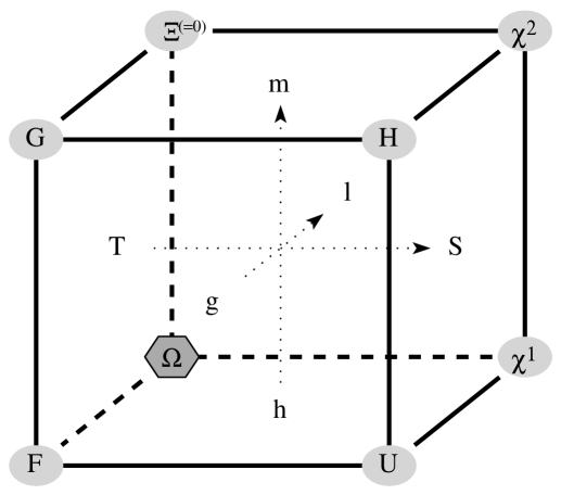
Figure 1: Born diagram. Corners correspond to thermodynamic potentials: the grand potential $\Omega$, the free energy $F$, the internal energy $U$, the enthalpy $H$, the free enthalpy $G$, the potential $\Xi$ (which vanishes for a homogeneous system), as well as two rarely used potentials $\chi^{1}$ and $\chi^{2}$. Sides of the cube correspond to thermodynamic variables: $T$, $S$, $g$, $l$, $h$ and $m$. Opposite sides are conjugate to each other, and associated with each conjugate pair is a dotted “basis vector.” Each corner is a function of the adjacent sides; e.g., the enthalpy $H$ is a function of $\{S,g,m\}$. Their conjugates $\{T,l,h\}$ can be obtained from $H$ by partial differentiation, the sign depending on whether the requested conjugate variable is at the head ($-$) or tail ($+$) of a basis vector; e.g., $T=+\partial H/\partial S$. One can go from one corner to the next by moving parallel or antiparallel to a basis vector, thereby (i) changing variables such as to get the correct dependence of the new potential, and (ii) adding (if moving parallel) or subtracting (if moving antiparallel) the product of the conjugate variables that are associated with the basis vector. For instance, in order to obtain the free enthalpy $G$ from the enthalpy $H$ one (i) uses $T=+\partial H/\partial S$ to solve for $S(T,g,m)$, since the free enthalpy will be a function of $\{T,g,m\}$ rather than $\{S,g,m\}$; and then (ii) subtracts the product $TS$ to get $G(T,g,m)=H(S(T,g,m),g,m)-TS(T,g,m)$. This procedure is known as a Legendre transformation. Successive application allows one to calculate all thermodynamic potentials from the grand potential $\Omega$ and hence, ultimately, from the partition function $Z$.

When a large system is physically divided into several subsystems then in these subsystems the thermodynamic variables generally take values that differ from those of the total system. In the special case of a homogeneous system all variables of interest can be classified either as extensive –varying proportionally to the volume of the respective subsystem– or intensive –remaining invariant under the subdivision of the system. Examples for the former are the volume itself, the internal energy or the number of particles; whereas amongst the latter are the pressure, the temperature or the chemical potential. In general, if a thermodynamic variable is extensive then its conjugate is intensive, and vice versa. If we assume that the temperature and the $\{l^{a}\}$ are intensive, while the $\{h^{b}\}$ and the grand potential are extensive, then

$$\Omega_{\rm hom}(T,l^{a},\tau h^{b})=\tau\cdot\Omega_{\rm hom}(T,l^{a},h^{b})\quad\forall\quad\tau>0$$ (87)

and hence

$$\Omega_{\rm hom}=-\sum_{b}m_{b}h^{b}\quad.$$ (88)

This implies the Gibbs-Duhem relation

$$S{d}T-\sum_{a}g_{a}{d}l^{a}-\sum_{b}h^{b}{d}m_{b}=0\quad.$$ (89)

For an ideal gas in the grand canonical ensemble, for instance, we have the temperature $T$ and the chemical potential $\{l^{a}\}=\{-\mu\}$ intensive, whereas the volume $\{h^{b}\}=\{V\}$ and the grand potential $\Omega$ are extensive; hence

$$\Omega_{\rm i.gas}(T,\mu,V)=-p(T,\mu)\,V\quad.$$ (90)

2.5 Correlations

Arbitrary expectation values $\langle A\rangle_{\rho}$ in the macrostate (54) or (56), respectively, depend on the Lagrange multipliers $\{\lambda^{a}\}$ as well as –possibly– on other parameters $\{h^{b}\}$. If the Lagrange multipliers vary infinitesimally while the $\{h^{b}\}$ are held fixed, the expectation value $\langle A\rangle_{\rho}$ changes according to

$${d}\langle A\rangle_{\rho}=-\sum_{a}\langle\delta G_{a};A\rangle_{\rho}{d}\lambda^{a}\quad.$$ (91)

Here $\langle;\rangle_{\rho}$ is the canonical correlation function with respect to the state $\rho$:

$$\langle A;B\rangle_{\rho}:=\int d{\bf{\pi}}\,\rho({\bf{\pi}})A({\bf{\pi}})^{*}B({\bf{\pi}})$$ (92)

in the classical case or

$$\langle A;B\rangle_{\rho}:=\int_{0}^{1}{d}\nu\,\mbox{tr}\left[\hat{\rho}^{\nu}\hat{A}^{\dagger}\hat{\rho}^{1-\nu}\hat{B}\right]$$ (93)

in the quantum case, respectively. The observable $\delta G_{a}$ is defined as

$$\delta G_{a}:=G_{a}-\langle G_{a}\rangle_{\rho}\quad.$$ (94)

The correlation matrix

$$C_{ab}:=\langle{\delta G_{a};\delta G_{b}}\rangle_{\rho}=-\left({\partial g_{b}\over\partial\lambda^{a}}\right)_{\lambda,h}=\left({\partial^{2}\over\partial\lambda^{a}\partial\lambda^{b}}\ln Z\right)_{\lambda,h}$$ (95)

thus relates infinitesimal variations of $\lambda$ and $g$:

$${d}g_{b}=-\sum_{a}{d}\lambda^{a}C_{ab}\quad,\quad{d}\lambda^{a}=-\sum_{b}{d}g_{b}(C^{-1})^{ba}\quad.$$ (96)

The subscripts $\lambda,h$ of the partial derivatives indicate that they must be taken with all other $\{\lambda^{a}\}$ and all $\{h^{b}\}$ held fixed. Returning to our example of the ideal quantum gas, we immediately obtain from (79) the correlation of occupation numbers

$$\langle{\delta N_{i};\delta N_{j}}\rangle_{\rho}=-{\partial n_{j}\over\partial\alpha^{i}}=\delta_{ij}\,n_{i}(1\pm n_{i})\quad.$$ (97)

3 Linear Response

3.1 Liouvillian and Evolution

The dynamics of an expectation value $\langle A\rangle_{\rho}$ is governed by the equation of motion

$${d\langle A\rangle_{\rho}\over dt}=\langle i{\cal L}A\rangle_{\rho}+\left\langle{\partial A\over\partial t}\right\rangle_{\rho}\quad.$$ (98)

Here we have allowed for an explicit time-dependence of the observable $A$. Classically, the Liouvillian ${\cal L}$ takes the Poisson bracket with the Hamilton function $H({\bf\pi})$,

$$i{\cal L}=\sum_{j}\left({\partial H\over\partial P_{j}}\,{\partial\over\partial Q^{j}}-{\partial H\over\partial Q^{j}}\,{\partial\over\partial P_{j}}\right)$$ (99)

in canonical coordinates ${\bf\pi}=\{Q^{j},P_{j}\}$; whereas in the quantum case it takes the commutator with the Hamilton operator $\hat{H}$,

$$i{\cal L}=(i/\hbar)\,[\hat{H},*]\quad.$$ (100)

An observable $A$ for which $i{\cal L}A+\partial A/\partial t=0$ is called a constant of the motion; a state $\rho$ for which ${\cal L}\rho=0$ is called stationary. Only for a stationary $\rho$ the Liouvillian is Hermitian with respect to the canonical correlation function,

$$\langle A;{\cal L}B\rangle_{\rho}=\langle{\cal L}A;B\rangle_{\rho}\quad\forall\,A,B\quad.$$ (101)

The evolver ${\cal U}$ is defined as the solution of the differential equation

$${\partial\over\partial t}{\cal U}(t_{0},t)={i}{\cal U}(t_{0},t){\cal L}$$ (102)

with initial condition ${\cal U}(t_{0},t_{0})=1$. As long as the Liouvillian ${\cal L}$ is not explicitly time-dependent, the solution has the simple exponential form

$${\cal U}(t_{0},t)=\exp[{i}(t-t_{0}){\cal L}]\quad;$$ (103)

however, we shall not assume this in the following. The evolver determines –at least formally– the evolution of expectation values via

$$\langle A\rangle_{\rho}(t)=\langle{\cal U}(t_{0},t)A\rangle_{\rho}(t_{0})\quad.$$ (104)

Multiplication with a step function

$$\theta(t-t_{0})=\left\{\begin{array}[]{ll}0&:\,t\leq t_{0}\\ 1&:\,t>t_{0}\end{array}\right.$$ (105)

yields the so-called causal evolver

$${\cal U}_{<}(t_{0},t):={\cal U}(t_{0},t)\cdot\theta(t-t_{0})$$ (106)

(where ‘$<$’ symbolizes ‘$t_{0}<t$’) which satisfies another differential equation

$${\partial\over\partial t}{\cal U}_{<}(t_{0},t)={i}{\cal U}_{<}(t_{0},t){\cal L}+\delta(t-t_{0})\quad.$$ (107)

If a (possibly time-dependent) perturbation is added to the Liouvillian,

$${\cal L}^{(V)}:={\cal L}+{\cal V}\quad,$$ (108)

then the perturbed causal evolver ${\cal U}^{(V)}_{<}$ is related to the unperturbed ${\cal U}_{<}$ by an integral equation

$${\cal U}^{(V)}_{<}(t_{0},t)={\cal U}_{<}(t_{0},t)+\int_{-\infty}^{\infty}{d}t^{\prime}\,{\cal U}^{(V)}_{<}(t_{0},t^{\prime})\,{i}{\cal V}(t^{\prime})\,{\cal U}_{<}(t^{\prime},t)\quad.$$ (109)

Iteration of this integral equation –re-expressing the ${\cal U}^{(V)}_{<}(t_{0},t^{\prime})$ in the integrand in terms of another sum of the form (109), and so on– yields an infinite series, the terms being of increasing order in ${\cal V}$. Truncating this series after the term of order ${\cal V}^{n}$ gives an approximation to the exact causal evolver in $n$-th order perturbation theory.

3.2 Kubo formula

The Kubo formula describes the response of a system to weak time-dependent external fields $\phi^{\alpha}(t)$. Before $t=0$ the external fields are zero and the system is assumed to be in an initial equilibrium state

$$\rho(0)={1\over Z}\exp\left(-\sum_{a}\lambda^{a}G_{a}[0]\right)$$ (110)

characterized by some set $\{G_{a}[0]\}$ of constants of the motion at zero field (and with the a priori distribution $\sigma$ taken to be uniform). Then the external fields are switched on:

$$\phi^{\alpha}(t)=\left\{\begin{array}[]{ll}0&:\,t\leq 0\\ \phi^{\alpha}(t)&:\,t>0\end{array}\right.\quad.$$ (111)

How does an arbitrary expectation value $\langle A\rangle(t)$ evolve in response to this external perturbation? The general solution is

$$\langle A\rangle(t)=\langle{\cal U}^{[\phi]}_{<}(0,t)A\rangle_{0}\quad,$$ (112)

where $\langle\rangle_{0}$ stands for the expectation value in the initial equilibrium state $\rho(0)$. We assume that the observable $A$ does not depend explicitly on time or on the fields $\phi^{\alpha}(t)$. The Hamiltonian $H[\phi]$ and with it the Liouvillian ${\cal L}[\phi]$, on the other hand, generally do depend on the external fields. Provided the fields are sufficiently weak, the Liouvillian may be expanded linearly:

$${\cal L}[\phi(t)]\approx{\cal L}[0]+\sum_{\alpha}\left.{\partial{\cal L}[\phi]\over\partial\phi^{\alpha}}\right|_{\phi=0}\phi^{\alpha}(t)\quad.$$ (113)

The zero-field Liouvillian ${\cal L}[0]$ is assumed to be not explicitly time-dependent; the linear correction to it generally is, and may be regarded as a time-dependent perturbation ${\cal V}(t)$. Application of first order time-dependent perturbation theory then yields the evolver ${\cal U}^{[\phi]}_{<}$ in terms of ${\cal V}(t)$ and the zero-field evolver ${\cal U}_{<}$. Assuming for simplicity that $\langle A\rangle_{0}=0$ we thus find

$$\langle A\rangle(t)=\sum_{\alpha}\int_{-\infty}^{\infty}{d}t^{\prime}\,\left\langle{i}\left.{\partial{\cal L}[\phi]\over\partial\phi^{\alpha}}\right|_{\phi=0}{\cal U}_{<}(t^{\prime},t)A\right\rangle_{0}\phi^{\alpha}(t^{\prime})\quad.$$ (114)

With the help of the mathematical identity (prove it!)

$$\langle{i}{\cal L}[\phi]B\rangle_{0}=\sum_{a}\langle{i}{\cal L}[\phi]G_{a}[0];B\rangle_{0}\lambda^{a}\quad\forall\,\,B$$ (115)

we can also write

$$\langle A\rangle(t)=\sum_{\alpha}\int_{-\infty}^{\infty}{d}t^{\prime}\sum_{a}\lambda^{a}\left\langle{i}\left.{\partial{\cal L}[\phi]\over\partial\phi^{\alpha}}\right|_{\phi=0}G_{a}[0];{\cal U}_{<}(t^{\prime},t)A\right\rangle_{0}\phi^{\alpha}(t^{\prime})\quad.$$ (116)

In general, the constants of the motion depend explicitly on the external fields. They satisfy

$${\cal L}[\phi]G_{a}[\phi]=0\quad\forall\,\phi\quad,$$ (117)

yet generally ${\cal L}[\phi^{\prime}]G_{a}[\phi]\neq 0$ for $\phi^{\prime}\neq\phi$. Together with the Leibniz rule this implies

$$\left.{\partial{\cal L}[\phi]\over\partial\phi^{\alpha}}\right|_{\phi=0}G_{a}[0]=-{\cal L}[0]\left.{\partial G_{a}[\phi]\over\partial\phi^{\alpha}}\right|_{\phi=0}\quad,$$ (118)

which we use to obtain

$$\langle A\rangle(t)=-\sum_{\alpha}\int_{-\infty}^{\infty}{d}t^{\prime}\sum_{a}\lambda^{a}\left\langle{i}{\cal L}[0]\left.{\partial{G_{a}}[\phi]\over\partial\phi^{\alpha}}\right|_{\phi=0};{\cal U}_{<}(t^{\prime},t)A\right\rangle_{0}\phi^{\alpha}(t^{\prime})\quad.$$ (119)

The right-hand side of this equation has the structure of a convolution, so in the frequency representation we obtain an ordinary product

$$\langle A\rangle(\omega)=\sum_{\alpha}\chi_{\alpha}^{A}(\omega)\phi^{\alpha}(\omega)\quad.$$ (120)

The coefficient

$$\chi_{\alpha}^{A}(\omega)=-\sum_{a}\lambda^{a}\int_{0}^{\infty}dt\,\exp(i\omega t)\left\langle{i}{\cal L}[0]\left.{\partial{G_{a}}[\phi]\over\partial\phi^{\alpha}}\right|_{\phi=0};A(t)\right\rangle_{0}$$ (121)

with $A(t):={\cal U}_{<}(0,t)A$ is called the dynamical susceptibility. The above expression for the dynamical susceptibility is known as the Kubo formula.

3.3 Example: Electrical conductivity

The conductivity $\sigma^{ik}(\omega)$ determines the linear response of the current density $\vec{j}$ to a (possibly time-dependent) homogeneous external electric field $\vec{E}$. We identify

$$\phi^{\alpha}\to E_{i}\quad,\quad A\to j^{k}\quad,\quad\chi_{\alpha}^{A}(\omega)\to\sigma^{ik}(\omega)\quad.$$ (122)

Since a conductor is an open system with the number of electrons fixed only on average, its initial state must be described by a grand canonical ensemble: $\{G_{a}[\phi]\}\to\{H[\vec{E}],N\}$, with associated Lagrange parameters $\{\lambda^{a}\}\to\{\beta,-\beta\mu\}$. In principle, the formula for the conductivity then contains both $\partial H/\partial E_{i}$ and $\partial N/\partial E_{i}$; but the latter vanishes, and there remains only

$${\partial H\over\partial E_{i}}=-eQ^{i}\quad,$$ (123)

with $Q^{i}$ denoting the $i$-th component of the position observable and $e$ the electron charge. We use the general formula (121) for the susceptibility to obtain

$$\sigma^{ik}(\omega)=e\beta\int_{0}^{\infty}dt\,\exp(i\omega t)\langle{i}{\cal L}[0]Q^{i};j^{k}(t)\rangle_{0}\quad.$$ (124)

The current density is related to the velocity $V^{k}$ by

$$j^{k}=enV^{k}\quad,$$ (125)

where $n$ is the number density of electrons. Furthermore, ${i}{\cal L}[0]Q^{i}=V^{i}$. Hence the conductivity is proportional to the velocity-velocity correlation:

$$\sigma^{ik}(\omega)=e^{2}n\beta\int_{0}^{\infty}dt\,\exp(i\omega t)\langle V^{i};V^{k}(t)\rangle_{0}\quad.$$ (126)

This result is rather intuitive. In a dirty metal or semiconductor, for instance, the electrons will often scatter off impurities, thereby changing their velocities. As a result, the velocity-velocity correlation function will decay rapidly, leading to a small conductivity. In a clean metal with fewer impurities, on the other hand, the velocity-velocity correlation function will decay more slowly, giving rise to a correspondingly larger conductivity.