Simulations of a single membrane between two walls
using a Monte Carlo method

Abstract

Quantitative theory of interbilayer interactions is essential to interpret x-ray scattering data and to elucidate these interactions for biologically relevant systems. For this purpose Monte Carlo simulations have been performed to obtain pressure $P$ and positional fluctuations $\sigma$. A new method, called Fourier Monte-Carlo (FMC), that is based on a Fourier representation of the displacement field, is developed and its superiority over the standard method is demonstrated. The FMC method is applied to simulating a single membrane between two hard walls, which models a stack of lipid bilayer membranes with non-harmonic interactions. Finite size scaling is demonstrated and used to obtain accurate values for $P$ and $\sigma$ in the limit of a large continuous membrane. The results are compared with perturbation theory approximations, and numerical differences are found in the non-harmonic case. Therefore, the FMC method, rather than the approximations, should be used for establishing the connection between model potentials and observable quantities, as well as for pure modeling purposes.

]

I Introduction

Recent research on lipid bilayers[1] has contributed to the important biological physics goal of understanding and quantifying the interactions between membranes by providing high resolution x-ray scattering data. From these data the magnitude of fluctuations in the water spacing between membranes in multilamellar stacks is obtained. This enables extraction of the functional form of the fluctuational forces, originally proposed by Helfrich [2] for the case of hard confinement. For systems with large water spacings, the Helfrich theory has been experimentally confirmed [3]. For lecithin lipid bilayers, however, the water spacing is limited to $20\AA$ or less. For this important biological model system, our data show that a theory of soft confinement with a different functional form is necessary; this is not surprising because interbilayer interactions consist of more than hard-wall, i.e., steric interactions.

The theory of soft confinement is even more difficult than the original Helfrich theory of hard confinement. Progress has been made by modeling the stack of interacting flexible membranes by just one flexible membrane between two rigid walls[4, 5]. Even with this simplification, however, the theory involves an uncontrolled approximation using first order perturbation theory and a self-consistency condition in order that the interbilayer interaction may be approximated by a harmonic potential[5]. We have obtained inconsistent results when applying this theory to our data (unpublished). Possible reasons are (i) the theory is quantitatively inaccurate or (ii) the single membrane model is too simple. The immediate motivation for this paper is to test possibility (i).

In order to obtain accurate results for a system with realistic non-harmonic potentials, we use Monte-Carlo (MC) simulations. The particular MC method developed in this paper will be called the FMC method because it uses the Fourier representation for the displacement of the membrane rather than the customary pointwise representation, which will be called the PMC method. The main advantage of the FMC method is that the optimal step sizes do not decrease as more and more amplitudes are considered. In contrast, in PMC simulations, the optimal step sizes decrease as the inverse of the density of points in one dimension, because the bending energy becomes large when single particle excursions make the membrane rough. Because of this, relatively large moves of the whole membrane are possible with the FMC method, but not the PMC method. This produces rapid sampling of the whole accessible phase space, while respecting the membrane’s smoothness. The resulting time series have moderate auto-correlation times [6] that do not increase substantially as the membrane gets larger and/or more amplitudes are taken into account. Even though each Monte Carlo step takes longer, FMC still outperforms PMC by a wide margin. It then becomes possible to carry out substantial simulations on a standalone workstation rather than a supercomputer[7] and to obtain accurate results for a single membrane subject to realistic potentials with walls, and even for a stack of such membranes (to be described in a future paper) [8].

Section II defines the membrane model and the physical quantities simulated in the paper. Section III describes the FMC method and also gives some important details that are used to speed up the code. In Section IV the method is tested on an exactly solvable model, namely, one that has only harmonic interactions with the walls. This test also allows examination of the system properties and the convergence of FMC results for an infinitely large, continuous membrane. In section V the FMC method is applied to a single membrane with realistic, non-harmonic interactions with the walls. Section VI makes a detailed comparison of the FMC method and the standard PMC method. This section shows that the FMC method not only converges faster to average values for continuous membranes, but also gives smaller stochastic errors. Finally, section VII compares simulation results with those obtained using the analytic first-order theory of Podgornik and Parsegian[5] and from experiment[1].

II Single Membrane System

FIG. 1.: A fluctuating single membrane, constrained between two hard walls.

At the atomic scale a lipid membrane is composed of complex lipid molecules and many simulations are performed at this scale [9, 10, 11]. However, for modeling the structure factor for low angle x-ray scattering (in contrast to modeling the form factor), it is customary and appropriate [12, 13, 14, 15] to model the membrane as an infinitely thin flexible sheet as shown in Fig.1.

The membrane undulates with instantaneous fluctuations in the $z$-direction, given by $u(x,y)$, subject to periodic boundary conditions. The model energy $W$ is a sum of bending energy with a bending modulus $K_{c}$ and an energy of interaction with the walls,

$$W=\frac{K_{c}}{2}\int({\Delta}u)^{2}dx\ dy+\int w_{a}(u)dx\ dy.$$ (1)

Since each wall is a surrogate for a neighboring membrane in a stack, and since it is desired to obtain physical properties per membrane, the interaction potential is given by the average $w_{a}(u)=(V(a+u)+V(a-u))/2$ of the interactions $V$ with each wall and the corresponding volume of the system per membrane is then $aL^{2}$. For a separation $z$ between a wall and the membrane the interaction potential will be based on the standard form

$$V(z)=A\lambda e^{-z/\lambda}-\frac{H}{12{\pi}z^{2}},$$ (2)

where the first term on the right hand side is a repulsive hydration potential [5] and the last term is an approximate, attractive van der Waals potential. The divergence in the van der Waals potential as $z{\rightarrow}0$ in Eq.(2) is quite artificial; physically, it is masked by stronger steric repulsions at small $z$ [16]. This is corrected in this paper by including only a finite number of terms $m_{max}$ in a power series expansion of $1/z^{2}$ about $u=0$. It is shown later that a wide range of $m_{max}$ give nearly the same result, so $m_{max}$ is not a critical parameter and power series suffice to represent the van der Waals potential satisfactorily for the most probable values of $z$ but avoid including artificial traps near the walls. Other forms besides Eq.(2) can be treated as well.

The first important quantity, obtained directly from the simulation, is the mean square fluctuation ${\sigma}^{2}$ in the water spacing. In Fig.1, $\sigma^{2}=\overline{u^{2}(x,y)}$, where the average is over both space and time. The second physical quantity is the pressure $P$ that must be exerted on the walls to maintain the average water spacing $a$. The pressure is a sum of two components: $P_{1}$, caused by collisions and equal to a temporal average of a delta-function-like instantaneous pressure, and $P_{2}$, which is due to non-contact interactions with the walls, and that varies smoothly with time and position. A virial theorem argument can be used to compute $P_{1}$. The general result is

$$P = \left[\frac{N^{2}k_{B}T-2\bar{U}}{2aL^{2}}-\frac{1}{2aL^{2}}\overline{\int u\frac{{\partial}w}{{\partial}u}dx\ dy}~{}\right]-$$ (4)

$$\overline{\frac{{\partial}w(u,a)}{{\partial}a}},$$

where $P_{1}$ is the term in square brackets. The relative importance of $P_{1}$ and $P_{2}$ depends on the potential. If the potential is completely steric (hard wall), then $P_{2}=0$. However, we have found that for the more realistic potentials considered in this paper $P_{1}$ is very small compared to $P_{2}$ because there are very few hard collisions.

III Fourier Monte Carlo (FMC) Method

The membrane displacement $u(x,y)$ is represented by its Fourier amplitudes $u(\vec{Q})$, where $\vec{Q}=(2{\pi}m/L,2{\pi}n/L)$, $N$ is the total number of modes in each dimension and $-N/2+1{\leq}m,n{\leq}N/2$. Reality of the displacement $u(x,y)$ is guaranteed by requiring $u(-{\vec{Q}})=u^{\ast}({\vec{Q}})$. Also, note that $u(\vec{Q}=0){\neq}0$ allows the center of gravity to fluctuate away from the midplane between the walls.

Using the standard Metropolis algorithm, the simulation attempts to vary one Fourier amplitude, picked randomly, at a time. The initial step sizes, which depend upon $\vec{Q}$, are determined using a simplified form of the analytic theory [5]. After a certain number of Monte Carlo steps (MCS), step sizes are adjusted using Dynamically Optimized Monte-Carlo(DOMC) [17]. Step size optimization results in an acceptance-rejection ratio of about 1/2, thereby minimizing the autocorrelation time $\tau$. In practice, because the initial values are already based on a reasonably good approximation, DOMC adjustment does not significantly improve the efficiency.

The change in bending energy in Eq.(1) after attempting a step in $u(\vec{Q})$ is $K_{c}L^{2}Q^{4}/2$ times the change in $|u(\vec{Q}|^{2}$, which requires little time to compute. In contrast, calculating the change in the interaction energy with the walls requires a real space representation of $u(x,y)$. However, it is not necessary to use a fast Fourier transform (FFT) routine because the linearity of the Fourier transform requires only recomputing one Fourier term in order to update $u(x,y)$. The time this takes is only $O(N^{2})$ compared to $O(N^{2}\ln N)$ for a standard FFT routine. Incremental addition errors are negligible for the longest runs when double precision is used; alternatively, one could perform FFT at long intervals to control such an error. The natural choice is made to approximate the interaction integral over the membrane by a sum over a set of equally spaced points $(Li/N,Lj/N)$, with $0{\leq}i,j<N$.

IV Harmonic Interactions and Finite-size Scaling

To test the simulation code and investigate convergence to an infinite, continuous membrane, it is useful to consider a harmonic interaction energy. It is also useful to relate the parameters in the harmonic potential to those in Eq.(1) by expanding $w_{a}(u)$ to second order about $u=0$,

$$w_{a} = A{\lambda}\exp(-a/\lambda)\left(1+\frac{z^{2}}{2\lambda^{2}}\right)-$$ (6)

$$-\frac{H}{12{\pi}a^{2}}\left(1+3\frac{z^{2}}{\lambda^{2}}\right),$$

so that the realistic Eq.(1) then takes the completely harmonic form

$$W_{0} = \frac{K_{c}}{2}\int({\nabla}^{2}u(r))^{2}d^{2}r+$$ (8)

$$\frac{B(a)}{2}\int u^{2}(r)d^{2}r+w_{0}(a)L^{2}.$$

where $B=(A/\lambda)e^{-a/\lambda}-H/(2{\pi}a^{4})$ and $w_{0}(a)=A{\lambda}e^{-a/\lambda}-H/(12{\pi}a^{2})$. The exact solution (valid for finite $L$ and $N/L$) for this harmonic model is

$$\sigma^{2}=\frac{T}{L^{2}}\sum_{q_{x},q_{y}}\frac{1}{K_{c}(q_{x}^{2}+q_{y}^{2})^{2}+B},$$ (9)

and

$$P=Ae^{-a/\lambda}\left[1+\frac{\sigma^{2}}{2\lambda^{2}}\right].$$ (10)

Equations (9) and (10) are useful in two ways. First, the harmonic approximation given by Eq.6 is good if $\sigma{\ll}\lambda$. That provides a test of the correctness of the code, which is written for the general case of realistic potentials and can then be applied when $\sigma{\ll}\lambda$. As an example, consider a membrane with parameters $N=4$, $L=700\AA$ and a non-harmonic potential with $A=1$, $H=100$ ($m_{max}=2$), $\lambda=10\AA$, $K_{c}=1$, $T=323K$, $a=20\AA$, where [18] gives the units for $A$, $H$ and $K_{c}$ used in this paper. The simulation gives $\sigma=0.3394{\pm}0.0004\AA$ and $P=1.2877{\cdot}10^{7}{\pm}200erg/cm^{3}$. In this case, $\sigma_{exact}=0.33954\AA$, and

$$P = Ae^{-a/\lambda}\left[1+\frac{\sigma^{2}}{2\lambda^{2}}\right]-\frac{H}{6{\pi}a^{3}}\left[1+6\frac{\sigma^{2}}{\lambda^{2}}\right]=$$ (12)

$$1.28774{\cdot}10^{7}erg/cm^{3},$$

again showing that simulation results are precise.

The second usage of Eqs. (9) and (10) is to obtain $\sigma$ and $P$ as functions of $N$ and $L$ through the finite sums over $\vec{Q}$. Simulations are always done with a finite number of Fourier amplitudes and a finite-sized membrane. However, real membranes are continuous and the relevant size may be larger than $1{\mu}m$. So it is important to see how the results for finite systems can be used to obtain quantities for dense ($N{\rightarrow}\infty$) and large ($L{\rightarrow}\infty$, $N/L=const$) systems. Eqs. (9) and (10) can be used to compute $\sigma(N,L)$ and $P(N,L)$ numerically to examine the asymptotic behavior of these functions. The result of such analysis is an asymptotic relation

$$\sigma{\approx}\sigma_{\infty}-C_{1}\left(\frac{L}{N}\right)^{2}-C_{2}\frac{1}{L^{2}},$$ (13)

where typically $C_{1}\sim 10^{-5}\AA^{-1}$ and $C_{2}\sim 10^{3}\AA^{3}$. The variability caused by the $C_{2}$ term is very small; typically about 0.2% when $L{\geq}700\AA$. However, the $C_{1}$ term causes $\sigma$ for a finite membrane to vary with $N$ as much as 20%.

V Obtaining Results for Realistic Interaction Potentials

Table I shows results for two selected non-harmonic potentials and a variety of sizes. One may first note that the autocorrelation times $\tau_{\sigma^{2}}$ and $\tau_{P}$ are nearly constant with system size. Next, convergence with increasing $N$ and constant $L$ is shown in Fig.2 when the vdW interaction is absent. This behavior is similar to that of a harmonic interaction. The limiting values can be estimated by fitting the curve $y=y_{\infty}+C_{2}/N^{2}+C_{3}/N^{3}$. The fits, shown as solid lines on Fig.2, lead to $\sigma_{\infty}=4.394{\pm}0.004\AA$ and $P_{\infty}=202400{\pm}700erg/cm^{3}$.

TABLE I.: Representative simulation results for two interactions.

N	$L[\AA]$	$\sigma[\AA]$	$P[\frac{erg}{cm^{3}}]$	MCS,$10^{3}$	$\tau_{\sigma^{2}}$	$\tau_{P}$
$A=1$, $H=0$, $K_{c}=1$ [18], $\lambda=1.8\AA$, $T=323K$, $a=20\AA$
4	700	4.0774${\pm}$0.0018	123010${\pm}$170	500	1.59	1.35
6	700	4.2767${\pm}$0.0034	156100${\pm}$400	100	1.44	1.18
8	700	4.3376${\pm}$0.0028	173700${\pm}$400	100	1.19	0.96
8	700	4.3366${\pm}$0.0013	173470${\pm}$170	500	1.21	0.98
12	700	4.359${\pm}$0.008	187000${\pm}$1300	10	1.16	0.97
16	700	4.3792${\pm}$0.0034	193800${\pm}$600	50	1.08	0.88
24	700	4.3864${\pm}$0.0024	197920${\pm}$430	30	0.946	0.768
32	700	4.399${\pm}$0.011	201500${\pm}$1900	6260	1.43	1.41
32	700	4.3976${\pm}$0.0030	200600${\pm}$500	20000	0.955	0.741
$A=1$, $H=3$, $m_{max}=4$, $K_{c}=0.1$, $\lambda=1.4\AA$, $T=323K$, $a=17\AA$
4	350	6.0902${\pm}$0.0027	28000${\pm}$900	500	2.46	1.03
6	525	6.1097${\pm}$0.0029	34400${\pm}$900	200	2.74	0.96
8	700	6.1225${\pm}$0.003	38500${\pm}$1000	100	2.7	0.97
12	1050	6.128${\pm}$0.005	40800${\pm}$1500	20	2.73	1.05
16	1400	6.1270${\pm}$0.0026	40000${\pm}$600	30	2.35	0.86
32	2800	6.136${\pm}$0.003	42000${\pm}$600	6	2.65	0.89

FIG. 2.: $\sigma$ and $P$ vs. $1/N^{2}$ for $A=1$, $H=0$, $\lambda=1.8\AA$, $a=20\AA$, $K_{c}=1$, $T=323K$ and $L=700\AA$.

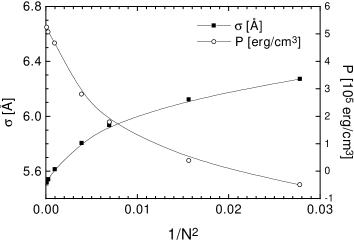
FIG. 3.: $\sigma$ and $P(1/N^{2},L=const=700\AA)$ for $A=1$, $H=3$, $m_{max}=4$, $\lambda=1.4$, $a=17$ and $K_{c}=0.1$. The lines are drawn to guide the eye.

Unfortunately, one does not obtain the same asymptotic behavior as in Fig.2 when the attractive force is large enough that the total potential has a maximum rather than a minimum when in the middle of the space between the walls. For instance, when $H{\neq}0$, $\sigma$ first decreases with $N$, although later it gradually levels off and appears to have a minimum. It is interesting that, while $\sigma$ may change in an unexpected way as $N$ increases, for the interaction considered, the pressure is still a smooth quasi-linear function of $1/N^{2}$ ($N{\rightarrow}\infty$), as shown in Fig. 3, and its limiting value as $N{\rightarrow}\infty$ can still be estimated by extrapolation. Despite these variations in convergence behavior, the associated changes in $\sigma$ become very small and are certainly less than the desired accuracy of 1-2%, so we suggest that it is sufficient to increase $N$ only to the point where further increases result in changes in $\sigma$ and $P$ that are less than the target precision.

The other variable that is potentially significant is the size of the membrane. Any physical quantity may depend on how large the membrane is, attaining a certain limiting value as $L{\rightarrow}\infty$. By increasing $L$ while keeping the “density” $N/L=const$, the membrane size is determined for which $\sigma$ and $P$ approach their limiting values sufficiently closely. As in the case of harmonic interaction, the changes in these quantities are relatively small as $L$ is increased. Indeed, when there is no attractive force, the changes are so small that they cannot be resolved reliably even when the estimated statistical errors are of order of $3{\cdot}10^{-3}\AA$. When the interaction is smaller, the trends become more pronounced and similar to those seen for the harmonic potential. An example is given in Fig.4 which shows that for a moderate sized membrane the results approach smoothly and closely those for an infinite membrane($L{\rightarrow}\infty$). For $L=700\AA$ the difference between the estimated limiting value of $\sigma$ and the observed one at $700\AA$ is less than 0.5%, while for the pressure the same difference is less than 5% which is about the same as the experimental uncertainty in $P$.

FIG. 4.: $\sigma$ and $P$ vs. $1/L^{2}$ with $N/L=8/700\AA$ for $A=1$, $H=3$, $K_{c}=0.1$ [18], $m_{max}=4$, $\lambda=1.4$ and $a=17$.

In summary, of the two factors that could affect convergence of simulation results, i.e. $N$ and $L$, $N$ is most important. $L$ is therefore fixed, typically at $700\AA$. $N$ is increased until the changes in quantities of interest are less than the target precision. We then fit a simple function such as $y=y_{\infty}+c_{2}/N^{2}+c_{3}/N^{3}$ to the sequence of finite $N$ results to estimate $y_{\infty}$.

VI Comparison of FMC and Standard PMC Methods

A Basics of the PMC Simulation Method

The standard way to simulate membranes [7] will be called the pointwise MC (PMC) method in which the potential of the system is given in discretized form

$$W = \frac{K_{c}}{2}\frac{N^{2}}{L^{2}}\sum_{ij}(\sum_{nn}u-4u_{ij})^{2}+$$ (15)

$$\frac{L^{2}}{N^{2}}\sum_{ij}w(u_{ij}),$$

where $\sum_{nn}u$ is the sum of displacements of nearest neighbors of site $(i,j)$. For a harmonic potential, $w(u)=w_{0}+Bu^{2}/2$, and for periodic boundary conditions the exact solution for the mean square displacement is

$$\sigma^{2} = \frac{k_{B}T}{L^{2}}\sum_{\vec{Q}}(B+4K_{C}\frac{N^{4}}{L^{4}}(\cos(Q_{x}\frac{L}{N})+$$ (17)

$$\cos(Q_{y}\frac{L}{N})-2)^{2})^{-1},$$

where $Q_{x,y}=2{\pi}n/L$, $-\frac{N}{2}+1{\leq}n{\leq}\frac{N}{2}$. As with the FMC method, such an exact solution is useful in checking correctness of the simulation code.

The standard Metropolis algorithm is used, moving one point at a time in the PMC method. To start the simulation, an effective B is estimated using perturbation theory[5]. It is then used in a formula that gives the mean-square fluctuation of a point (assuming harmonic potential) about its equilibrium position, determined by its environment:

$$\sigma_{local}=\sqrt{\frac{k_{B}T}{BL^{2}/N^{2}+20K_{c}N^{2}/L^{2}}}$$ (18)

Eq.(18) gives the initial step size. After a certain number of steps, DOMC[17] is used to compute the optimal step size, which is used thereafter. Some results using the PMC method are presented in Table II.

TABLE II.: Real space simulations of membranes with different density of points, constrained by a harmonic potential with $B=8.303{\cdot}10^{11}erg/cm^{4}$ obtained from $A=1$, $H=0$, $K_{c}=1$ [18], $\lambda=1.8\AA$, $a=20\AA$. $T=323K$, $L=700\AA$. Simulation lengths are measured in $10^{6}$ MCS.

N	$\sigma[\AA]$	MCS	MCS0.1%∗	$\tau_{\sigma^{2}}$
4	8.390${\pm}$0.005	1	0.41	4.36
6	8.481${\pm}$0.008	1	0.98	13.8
8	8.332${\pm}$0.031	0.2	2.77	41.9
8	8.347${\pm}$0.032	0.2	2.94	42.3
8	8.305${\pm}$0.010	2	2.73	39
12	8.073${\pm}$0.016	4	14.9	203
12	8.070${\pm}$0.015	4	14.6	198
16	8.00${\pm}$0.06	1	66	782
16	8.07${\pm}$0.06	1	59	709

^∗ A simulation of approximately such length would have to be done to attain 0.1% accuracy for $\sigma$.

B Comparison of the FMC and PMC methods

The time required to obtain a target error is one of the issues determining the viability of any simulation technique. It is impacted by two separate factors: the relative magnitude of random errors, and the speed at which various quantities, obtained for a finite system, converge to their values for the continuous infinite system. These factors are now considered in detail, to demonstrate the improvements of the FMC method.

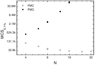
FIG. 5.: Variation with N of the simulation length $MCS_{0.1\%}$, required for 0.1% precision of $\sigma$, for a PMC simulation of a harmonic potential with $A=1$, $H=0$, $K_{c}=1$, $\lambda=1.8\AA$, $a=20\AA$, $T=323K$ and $L=700\AA$ and for an FMC simulation for a realistic model potential with the same parameters.

The random errors in estimated averages depend on the autocorrelation times of generated time series. These times are an indication of how “natural” the chosen basis is for the simulated system. In the case of harmonic interactions, the variables used by FMC are exactly independent and therefore it is possible to vary each of them separately over its whole range. Although they do become correlated for realistic interactions, one would still hope that their dependencies are not great, and so they still represent a good basis. For PMC simulations, however, the motion of any point is constrained by its environment, so one would expect the quality of time series to deteriorate as the “density” of the membrane and the importance of the local environment increase. These assertions are supported by Tables I and II, which show that for FMC the autocorrelation times remain roughly constant with increasing $N$, whereas for PMC ${\tau}_{\sigma}$ increases as $N^{4}$. A related question is how the simulation length (in MCS) required to obtain a certain accuracy (chosen to be 0.1%) varies with N. A straight line fit to $\ln(MCS_{0.1\%})$ vs. $\ln N$ dependence for PMC has a slope of approximately 4 (Fig.5). Therefore, the amount of time required to obtain $\sigma$ with the same precision grows as $N^{6}$ for PMC method. A somewhat surprising result is that the length required to achieve a given error estimate with FMC decreases with N (Fig.5). The precise law governing this decrease is unclear because of the difficulty of estimating autocorrelation times; one guess, supported by the four points in the middle ($N=8$ through 24) is that the length decreases as $1/\sqrt{N}$; however, the hypothesis of the length staying asymptotically constant cannot be ruled out either. Because 1 MCS (for FMC) takes the amount of time $O(N^{4})$, the computational complexity of the process generated by a Fourier-space simulation is only $N^{3.5}$ or $N^{4}$, assuming that the same error estimate is achieved. This is a significant improvement over the $N^{6}$ law for the real-space simulations.

The second factor favoring FMC concerns how closely the bending energy is approximated by the discrete approximation in Eq.(15). This can be evaluated by the exact result for $\sigma$ for a harmonic model. Fig.6 shows that one requires larger $N$ to obtain the same precision with the discrete approximation to the bending energy required by the PMC method in Eq.(15) than for the true continuum model that can be treated naturally by the FMC method.

FIG. 6.: Exactly computed $\sigma(N,L=700\AA)$ for Fourier-space (Eq.(9)) and real-space (Eqs.(15) and (17)) models of a harmonic potential with $B=8.303{\cdot}10^{11}erg/cm^{4}$. The other parameters are $K_{c}=1$, $T=323K$ and $L=700\AA$.

A specific example illustrates the preceding principles and also gives some typical computer times for these simulations. The example is the harmonic model with parameters given in Fig.6. For the PMC simulation, $N=46$ was chosen so that $\sigma_{exact}(46,L=700\AA)=7.7898$ was within 0.5% of its value $7.7478\AA$ for a continuous membrane. A simulation of 800,000 MCS took 9.5 hours on an SGI workstation with MIPS R5000 1.0 CPU and 128 Mb of RAM, running IRIX 6.2 and resulted in ${\sigma}=7.33{\pm}0.19$. So, 9.5 hours were insufficient to obtain $\sigma$ with 0.5% accuracy, and about $9.5{\cdot}(0.19/(0.005{\cdot}7.75))^{2}{\approx}229$ hours would be required to achieve that precision. Turning to FMC, for $N=16$ the exact $\sigma=7.7111\AA$. A run of 10,000 MCS yielded $\sigma=7.7184{\pm}0.0165$ and required only 240 seconds on the same computer as the PMC simulation. One may also compare the time it takes to obtain the same estimates of random errors for the same $N$ for the two methods. To do this, $N=16$ and a target error of about 1% were chosen for the same interaction as before. A PMC simulation for 300000 MCS took 1174 seconds on an SGI workstation with a similar configuration to the one used in the previous test and resulted in $\sigma=8.032{\pm}0.082\AA$ ($\tau_{E}=14.7$, $\tau_{\sigma^{2}}=441$), a slightly bigger error than desired. In contrast, an FMC simulation (also with $N=16$) for 2000 MCS took only 63 seconds on the same computer, and resulted in $\sigma=7.674{\pm}0.070\AA$ ($\tau_{E}=2.19$, $\tau_{\sigma^{2}}=1.44$), the random error in $\sigma$ now being slightly better than the target. So, in addition to a much faster convergence of the expected value to one for a continuous membrane, the FMC method is also the faster one to obtain a given estimate of stochastic errors.

VII Results and Implications

A Distribution of the membrane displacements

The functional form of the probability density function (pdf) is a central assumption in the perturbation theory [5]. Also, the behavior of the pdf near the walls is significant in discussing the formal divergence of the van der Waals potential and the importance of the hard wall collision pressure $P_{1}$. If the pdf does not decay to zero sufficiently quickly near the walls, then the value of $m_{max}$ used in the power series expansion would be a sensitive parameter and one would expect many hard collisions with the walls. The inset to Fig.7 shows that the pdf decays to zero near the walls in much the way that is postulated by theory[5]. This is consistent with our results that $P_{1}$ is small and $m_{max}$ is an insensitive parameter. This latter point is explicitly illustrated in Fig.8 which shows that the results for $\sigma$ plateau for $6<m_{max}<40$; a similar plateau occurs for $P$. Finally, Fig.7 shows that, away from the walls, the pdf is noticeably different from the theoretically assumed pdf[5] and it is generally different from a Gaussian.

FIG. 7.: Membrane pdf for a realistic constraining potential. $A=0.2$, $H=0.5$, $\lambda=1.3\AA$, $m_{max}=3$, $T=323K$, $K_{c}=0.1$, $a=22\AA$, $N=32$ and $L=700\AA$. Also shown are the Gaussian pdf, corresponding to $\sigma=8.0196\AA$ and the approximate pdf for the case of pure steric constraint proposed in [5](Eq.(20)).

FIG. 8.: The relationship between the number of terms in the expansion approximating van der Waals potential and $\sigma$, for the parameter set $a=1$, $H=6$, $\lambda=1.8$, $K_{c}=0.2$, $T=323$, $a=13$, $L=700$. The line is drawn to guide the eye.

B $P$ and $\sigma$

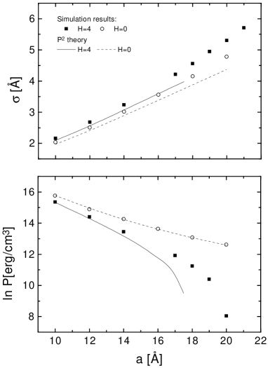
FIG. 9.: $\sigma(a)$ and $\ln P(a)$, obtained from a simulation for $A=1$, $H=4$, $\lambda=1.8$, $K_{c}=0.2$ and also for H=0 (all other parameters being the same) and corresponding results from the perturbation theory[5].

For any kind of interaction, the main results to compare to experiment are the relationships between $\ln P$ and $a$, and $\sigma$ and $a$. Figure 9 shows $\ln P$ and $\sigma$ for several values of $a$. Two interaction types are considered: $A=1$, $H=4$, $\lambda=1.8$, $K_{c}=0.2$ and the same set with $H=0$. These figures also show the results obtained from the first-order perturbation theory [5]. The largest differences with the simulations occur at larger $a$ and when $H$ is non-zero. In particular, the theory under-predicts the value of $a$ at $P=0$ when no osmotic pressure is applied. Overall, however, the theory predicts trends quite well.

C Comparison to Experiment

Recently, it has been proposed that the pressure due to fluctuations, $P_{fl}$, can be obtained from x-ray line shape data [1]. The derivation involves the use of harmonic Caille theory[12, 15], which yields

$$P_{fl}=-\left(\frac{4}{\pi}\frac{k_{B}T}{8}\right)^{2}\frac{1}{K_{c}}\frac{d{\sigma}^{-2}}{da},$$ (19)

where $\sigma$ is obtained from

$$\sigma^{2}={\eta}_{1}D^{2}/{\pi}^{2},$$ (20)

where $\eta_{1}$ is the Caille parameter determined by the line shape. The experimental data for three different lipids indicated that $P_{fl}$ could be represented by an exponential $exp(-a/{\lambda}_{fl})$, in agreement with the result of perturbation theory [5], but that ${\lambda}_{fl}$ was significantly greater than $2\lambda$ instead of exactly $2\lambda$ given by perturbation theory. Since neither the perturbation theory nor the harmonic interpretation of the data are necessarily correct, it is valuable to test these predictions using simulations.

Figure 10 shows two ways of obtaining $P_{fl}$ from the simulations. The first way uses the definition

$$P=P_{fl}+P_{b},$$ (21)

where $P$ is the total osmotic pressure and $P_{b}$ is the pressure with no fluctuations, i.e. for the membrane exactly in the middle of the space between the two walls with $u(x,y)=0$. The second way uses Eq.(19). Fig.10 shows that the simulated $P_{fl}$ can be reasonably represented by an exponential using either method of computation, thereby supporting both theory and experiment. Either method gives decay lengths ${\lambda}_{fl}$ that exceed $2\lambda$, thereby supporting experiment. The two results for $P_{fl}$ in Fig.10 do not, however, agree perfectly, and the discrepancy grows for larger values of $a$. This is not surprising because the harmonic approximation is better for small $a$ and progressively breaks down, especially when the bare potential no longer has a minimum at $z=0$. This discrepancy suggests that one should expect some error when subtracting $P_{fl}$ obtained from Eq.(19) from $P$ in Eq.(21) to obtain $P_{b}$, although the error is encouragingly small. Nevertheless, future work in this direction can employ simulations to correct this discrepancy and to allow a better estimate of $P_{b}$ from which $P_{h}$, $\lambda$ and $H$ are obtained [1].

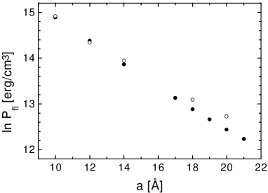
FIG. 10.: Simulation results for $P_{fl}$ vs. $a$ for $A=1$, $H=4$, $K_{c}=0.5$ [18], $\lambda=1.8\AA$. Solid circles show $P_{fl}$ obtained from Eq.(21) with a slope ${\lambda}_{fl}=4.1\AA$. Open circle show $P_{fl}$ obtained from Eq.(19) with a slope ${\lambda}_{fl}=4.6\AA$.

VIII Conclusions

This paper solves accurately a model of constrained single membrane fluctuations. The new FMC simulation method provides a way to simulate accurately, with modest computer resources, the pressure and mean square fluctuation of a simple membrane between two hard walls with realistic potentials. This method is clearly superior to the more conventional PMC simulation method. Used with typical values of interaction parameters, it supports the idea of the exponential decay of fluctuational pressure, lending credibility to a simplified interpretation of X-ray scattering data in [1]. Finally, the method, with minor modification, may be applied to studies of more complicated models, such as a stack of membranes or models of charged lipids and more sophisticated data analysis.

Acknowledgments: We thank Horia Petrache for useful discussions and acknowledge Prof. R. H. Swendsen for his illuminating expositions of Monte Carlo technique. This research was supported by the U. S. National Institutes of Health Grant GM44976.

REFERENCES

- [1] H. I. Petrache, N. Gouliaev, S. Tristram-Nagle, R. Zhang, R. M. Suter, and J. F. Nagle, submitted to Phys. Rev. E.
- [2] W. Helfrich, Z. Naturforsch. 33a, 305 (1978).
- [3] C. R. Safinya, E. B. Sirota, D. Roux and G. S. Smith, Phys. Rev. Lett. 62, 1134 (1989), although a considerable numerical discrepancy with MC simulations has remained unresolved, see, e.g., R. R. Netz, Phys. Rev. E 51, 2286 (1995).
- [4] D. Sornette and N. Ostrowsky, J. Chem. Phys. 84, 4062 (1986).
- [5] R. Podgornik and V. A. Parsegian, Langmuir 8, 557 (1992).
- [6] The duration of a simulation is measured in Monte-Carlo steps (MCS). 1 MCS is defined as such a sequence of “moves” that, on average, changes the variable corresponding to each degree of freedom once. One MCS is equivalent to changes of randomly chosen amplitudes for FMC simulations and for PMC simulations it is equivalent to moves of randomly chosen points. The auto-correlation times [19], denoted with subscripts referring to physical quantities are also measured in MCS.
- [7] R. Lipowsky, B. Zielinska, Phys. Rev. Letts., 62, 1572 (1989)
- [8] In contrast to the soft confinement regime, extensive simulations have been performed for single membranes and for short stacks in the hard confinement regime using the PMC method. Some general reviews include W. Janke, Int. J. Mod. Physics B 4, 1763 (1990), G. Gompper and M. Schick, Phase Transitions and Critical Phenomena, Vol. 16 (Academic Press, 1994), eds. C. Domb and J. L. Lebowitz and R. Lipowsky, Handbook of Biological Physics, Vol. I, Chapter 11 (Elsevier, 1995), eds. R. Lipowsky and E. Sackmann.
- [9] S. E. Feller, R. M. Venable and R. W. Pastor, Langmuir 13, 6555 (1997)
- [10] L. Perera, U. Essmann and M. L. Berkowitz, Progr. Colloid. Polym. Sci. 103, 107 (1997)
- [11] K. Tu, D. J. Tobias and M. L. Klein, Biophys. J. 69, 2558 (1995)
- [12] A. Caille, C. R. Acad. Sc. (Paris) Serie B 174, 891 (1972).
- [13] J. Als-Nielsen, J. D. Litster, R. J. Birgeneau, M. Kaplan, C. R. Safinya, A. Lindegaard-Anderson and R. Mathiesen, Phys. Rev. B 22, 312 (1980).
- [14] R. Holyst, Phys. Rev. A44, 3692 (1991).
- [15] R. Zhang, R. M. Suter and J. F. Nagle, Phys. Rev. E 50, 5047 (1994).
- [16] T. J. McIntosh, A. D. Magid, and S. A. Simon, Biochemistry 26, 7325 (1987).
- [17] D. Bouzida, S. Kumar and R. H. Swendsen, Phys. Rev. A, 45, 8894 (1992)
- [18] In this paper, the following units for the interaction parameters will be used for brevity: , , .
- [19] H. Müller-Krumbhaar and K. Binder, J. Stat. Phys, 8, 1 (1973)