Raman cooling of atoms below the gravitational limit

Abstract

Raman cooling of non-zero-spin atoms in the presence of gravitational and external magnetic fields is investigated. The magnetic field is adjusted so as to compensate for the gravitational force acting on ground-state atoms. The dark state (DS) is created and supported in momentum space with additional velocity-selective two-photon transitions. The minimum allowed temperature is found to be determined only by the width of velocity selection and therefore can be much less than the gravitational limit. A complete set of analytical formulas describing cooling of a dilute atomic sample is derived. They serve as the basis for numerical simulations which are carried out in the one-dimensional (1D) case.

I INTRODUCTION

Methods of laser cooling of atoms have progressed dramatically in recent years. There are three typical temperature scales characterizing various methods. The first one is specific to the most common scheme in which Doppler shift causes the radiation pressure force to be velocity dependent, thus damping atomic motion when the laser frequency is tuned below an atomic resonance. The minimum temperature $T_{D}$ for atoms cooled in such a way is known as the ”Doppler limit”. It is proportional to the natural width of the laser-driven transition $\gamma$ [1], $k_{B}T_{D}=\hbar\gamma/2$, and for the $D$ line of Na the Doppler limit is approximately 240 $\mu$K.

Schemes based on dissipation of atomic energy via interaction with the vacuum modes of electromagnetic field have a lower limit on the achievable temperature defined by the minimum of recoil energy which an atom obtains after spontaneous photon emission. The corresponding scale is known as the recoil limit $k_{B}T_{R}=(\hbar k)^{2}/2M$, where $k$ is the wave number of emitted light, and $M$ is the atomic mass. For Na it approximately equals to 1 $\mu$K.

To overcome this limit two subrecoil cooling methods have been developed and demonstrated: velocity selective coherent population trapping (VSCPT) [2] and Raman cooling [3]. Both methods imply the existence of the so-called dark state, which does not interact with light, has a long lifetime and occupies only a few modes in momentum space [4]. During the cooling cycle atoms diffuse into this state due to random recoil induced by spontaneous emission and accumulate in it. Since DS has a vanishing absorption rate of light, the final temperature is restricted not by the recoil limit but by the time of cooling which, however, cannot be greater than the lifetime of DS.

In the absence of Earth gravity, infinitely long cooling times would be possible. In practice the gravitational field pushes atoms from DS, reducing its lifetime dramatically. For any 3D configuration this defines the third characteristic temperature scale [5] $k_{B}T_{G}=Mg/k$, the gravitational limit. It lies below the recoil limit for most atoms, e.g., $T_{G}=0.07T_{R}$ for Rb, and $T_{G}=0.003T_{R}$ for Na.

Two ways are envisioned to prepare a stable quantum state of matter in the gravitational field: to bound particles or to suspend them free in an inhomogeneous magnetic field using Stern-Gerlach effect. In the first approach atoms are confined by a conservative trapping potential which can be realized, e.g., in a far-off-resonance or a dipole trap, where an intensity gradient provides a spatially dependent ac Stark shift. In momentum space, up to now only the existence of an approximate dark state has been demonstrated [6], characterized by a decay rate in a special 1D atomic and laser field configuration much smaller than that of all other states in the trap. The finite lifetime of approximate DS evidently restricts the cooling possibilities in a trap, leaving the question about going below the gravitational limit to be clarified. However, a scheme [7] which is based on the creation of a dark state in position space with the help of an appropriate spatial profile of the cooling laser, e.g., in a doughnut mode, seems to be much more efficient, allowing to cool a significant fraction of atoms to the ground state of the trapping potential.

Another approach may be applied to atoms possessing a magnetic moment. Superimposing a weakly inhomogeneous magnetic field onto the path of pre-polarized particles and appropriately adjusting the field gradient it is possible to compensate the effects of gravity for a definite internal atomic state. However, the magnetic field induces spatially dependent shifts of the Zeeman levels, which lead to unwanted residual excitation from the DS in the framework of any traditional subrecoil cooling method. Moreover, in the case of VSCPT the dark state cannot be an eigenvector of the total Hamiltonian since only one of the internal states forming the superposition which is not coupled to the laser field may escape gravity. Thus, both VSCPT and Raman cooling mechanisms in their standard form are incompatible with the last approach.

To resolve this problem we suggest a modification of Raman cooling method, in which the ground-level atoms are made motionally free with the Stern-Gerlach effect and the DS is created and supported in momentum space of these atoms with additional velocity-selective two-photon transitions. The transitions couple external momentum states of the same ground internal level and are organized in such a manner that DS cyclically occupies different thin sets of velocity modes while remaining unreachable for the Raman excitation-repumping pulse sequences at all times.

In Sec.  II a detailed qualitative treatment of the suggested scheme is given. For reasonable experimental conditions all the stages of the scheme admit analytical descriptions which are presented in Sec.  III - Sec.  V. Specifically, the formulas describing a coherent two-photon transition when an atom is placed in a superposition of two plain electromagnetic waves with arbitrary directions of the wave vectors are presented in Sec. III. In Sec.  IV Raman excitation to the closest hyperfine level is investigated in the regime in which the photon spontaneous emission may be neglected. Both the exact quadrature and convenient approximate expressions are derived. In Sec. V the optical pumping of atoms back to the ground state is considered for short times of light pulse, i.e., when the external potential field does not affect the atomic motion substantially. A numerical simulation of 100 cooling sequences in one dimension is given in Sec. VI. Section VII concludes with a summary of the obtained results.

II QUALITATIVE TREATMENT

Consider for definiteness an atom with a $J=\frac{1}{2}$ to $J=\frac{3}{2}$ transition, e.g., sodium or cesium. The magnetic field ${\bf{B}}({\bf{r}})$ applied to compensate the gravity is supposed to contain a homogeneous component ${\bf{B}}_{0}$ directed along the gravity acceleration ${\bf{B}}_{0}\uparrow\uparrow{\bf{g}}$. The remaining inhomogeneous part of the field ${\bf{B}}_{1}({\bf{r}})={\bf{B}}({\bf{r}})-{\bf{B}}_{0}$ should be small compared to this component,

$$|{\bf{B}}_{1}({\bf{r}})|\ll B_{0}=|{\bf{B}}_{0}|.$$ (1)

As we will see below, to fulfil this condition it is necessary to take $B_{0}$ in the range $10^{3}\div 10^{4}$ G. In practice such a field is strong enough to induce Zeeman shifts which considerably exceed the hyperfine splitting intervals $\sim\hbar\omega_{\rm HFS}$ (but not the multiplet ones). Therefore an internal atomic eigenstate $|J,I,M_{J},m_{I}\rangle$ may be well described using the set of quantum numbers consisting of the angular momenta of the electronic shell $J$ and the nucleus $I$, and their local projections $M_{J}$, $m_{I}$ on the direction of the magnetic field.

In the framework of perturbation theory, $|J,I,M_{J},m_{I}\rangle$ represents a combination of eigenstates $|J,I,M_{J},m_{I}\rangle^{(0)}$ related to the atomic Hamiltonian without the hyperfine interaction,

$$|J,I,M_{J},m_{I}\rangle= |J,I,M_{J},m_{I}\rangle^{(0)}+\frac{a}{2\mu_{B}g_{L}B_{0}}$$ (6)

$$\times\left\{[(J+M_{J})(J-M_{J}+1)]^{1/2}[(I+m_{I}+1)(I-m_{I})]^{1/2}\right.$$

$$\times|J,I,M_{J}-1,m_{I}+1\rangle^{(0)}$$

$$-[(J+M_{J}+1)(J-M_{J})]^{1/2}[(I+m_{I})(I-m_{I}+1)]^{1/2}$$

$$\times\left.|J,I,M_{J}+1,m_{I}-1\rangle^{(0)}\right\},$$

where $a$ is the hyperfine coupling constant ($a\propto\hbar\omega_{\rm HFS}$, e.g., for Na $a/\hbar=885.8$ MHz) and $g_{L}$ denotes the Lande factor. The corresponding energy eigenvalue is determined not only by the multiplet level $E_{J}$ but also by the magnetic field $B({\bf{r}})=|{\bf{B}}({\bf{r}})|$ and therefore is spatially dependent

$$E_{|J,I,M_{J},m_{I}\rangle}({\bf{r}})= E_{J}+aM_{J}m_{I}$$ (8)

$$+(\mu_{B}g_{L}M_{J}-\mu_{\rm nuc}m_{I})B({\bf{r}}),$$

where $\mu_{\rm nuc}$ is the nuclear magnetic moment. Because of the condition (1) such a spatial dependence, however, mainly arises from the longitudinal ($B^{\parallel}_{1}({\bf{r}})={\bf{B}}_{0}\cdot{\bf{B}}_{1}({\bf{r}})/B_{0}$), rather than the transverse (${\bf{B}}^{\perp}_{1}({\bf{r}})$) component of the vector ${\bf{B}}_{1}({\bf{r}})$, provided that the components are defined relative to ${\bf{B}}_{0}$. This is evident from the expression

$$B({\bf{r}})= \sqrt{\left[B_{0}+B^{\parallel}_{1}({\bf{r}})\right]^{2}+\left[{\bf{B}}^{\perp}_{1}({\bf{r}})\right]^{2}}$$ (10)

$$\simeq B_{0}+B^{\parallel}_{1}({\bf{r}})+\left[{\bf{B}}^{\perp}_{1}({\bf{r}})\right]^{2}/(2B_{0}),$$

where the term containing ${\bf{B}}^{\perp}_{1}({\bf{r}})$ is small and can be neglected. Consequently, by adjusting the gradient of the field $B^{\parallel}_{1}({\bf{r}})$ one can achieve translational invariance of the ground state $|1\rangle=|1/2,I,-1/2,I\rangle$ in three dimensions:

$$E_{|1\rangle}({\bf{r}})-M{\bf{g}}\cdot{\bf{r}}=\mbox{\rm const}.$$ (11)

For example, to balance the gravitational force in this way for sodium it is necessary to create a gradient $\nabla B^{\parallel}_{1}({\bf{r}})=b_{1}{\bf{g}}/|{\bf{g}}|$, where $b_{1}=-4.033$ G$/$cm. This condition does not contradict the Maxwell equation $\nabla\cdot{\bf{B}}_{1}({\bf{r}})=0$, because variation of ${\bf{B}}^{\perp}_{1}({\bf{r}})$ is not restricted. Note also that the choice $B_{0}=10^{3}\div 10^{4}$ G maintains the condition (1) very well within a spatial region of the size $\sim 10$ cm.

All the other levels are affected by the residual external potential. In particular, after a transition from $|1\rangle$ to the neighboring state $|2\rangle=|1/2,I,-1/2,I-1\rangle$ the atom experiences a force

$${\bf{f}}_{2}=\frac{M\mu_{\rm nuc}{\bf{g}}}{(1/2)\mu_{B}g_{L}+\mu_{\rm nuc}I}.$$ (12)

In our scheme, we use pulses of laser light at frequencies $\omega_{1}$ and $\omega_{2}$ which are roughly tuned to the $|1\rangle\to|3\rangle$ and $|2\rangle\to|3\rangle$ transitions, where $|3\rangle=|3/2,I,-3/2,I\rangle$ is an excited state with the lowest energy. The typical size $2L$ of atomic sample is restricted by the condition $L\ll a/(Mg)$, which allows to regard $E_{|3\rangle}({\bf{r}})$ as the closest to resonance excited level within the whole interaction domain. Indeed, the force ${\bf{f}}_{3}$ acting on the atoms in the state $|3\rangle$ may be estimated from Eqs.  (8) and (11) as $|{\bf{f}}_{3}|\sim Mg$. The maximal spatial shift of the level $\sim MgL$ which it induces is much less than the hyperfine splitting intervals ($MgL\ll a\sim\hbar\omega_{\rm HFS}$), and the hierarchy of detunings is retained. Therefore an atom initially in $|1\rangle$ or $|2\rangle$ state behaves as a three-level system with respect to the processes with stimulated emission of photons.

Since the atomic dipole momentum operator $\hat{\bf{d}}$ is diagonal in quantum numbers $I$ and $m_{I}$ in the basis $|J,I,M_{J},m_{I}\rangle^{(0)}$, the transitions which change $m_{I}$, e.g., $|2\rangle\to|3\rangle$, are allowed only due to hyperfine interaction, as is seen from Eq. (6). The value of any matrix element like $|\langle 3|\hat{\bf{d}}|2\rangle|$ is approximately $\propto\eta_{\rm HF}|\langle 3|\hat{\bf{d}}|1\rangle|$, where $\eta_{\rm HF}=a/(2\mu_{B}g_{L}B_{0})\ll 1$. As a consequence, the upper state $|3\rangle$ decays to the lower ones preferentially in the channel $|3\rangle\to|1\rangle$ (with the rate $\gamma$). This circumstance makes it possible to deal with an atom as a three-level system even if spontaneous photon emission takes place.

When the atom is irradiated with two laser beams at frequencies $\omega_{1}$ and $\omega_{2}$, the two-photon Raman transition from $|1\rangle\to|2\rangle$ has twice the Doppler sensitivity of a single-photon transition provided that $\omega_{1}-\omega_{2}\sim\omega_{\rm HFS}$ and the beam wave vectors ${\bf{k}}_{1}$, ${\bf{k}}_{2}$ are opposite [3]. However, if we take into account the force (12), a wide set of atomic momenta ${\bf{p}}$ may satisfy the resonance condition, as follows from the energy conservation:

$$\hbar\Delta_{1}-2{\bf{p}}\cdot{\bf{\Delta}}_{p}/M=\hbar\Delta_{2}-{\bf{f}}_{2}\cdot{\bf{r}}+2\Delta_{p}^{2}/M.$$ (13)

Here detunings $\Delta_{m}\equiv\omega_{m}+[E_{|m\rangle}(0)-E_{|3\rangle}(0)]/\hbar$, $m=1,2$, are defined in the center of atom-laser interaction region (${\bf{r}}=0$), ${\bf{\Delta}}_{p}=\hbar({\bf{k}}_{1}-{\bf{k}}_{2})/2$, and $\Delta_{p}=|{\bf{\Delta}}_{p}|$. The dip in the velocity dependence of absorption rate broadens so that the width of the trapping zone [8] becomes

$$\delta v\sim L|{\bf{f}}_{2}|/(2\Delta_{p}).$$ (14)

As a consequence, since the sample of unconfined particles considered in this paper may spread up to $L\sim 1$ cm during the cooling, the effective temperature of atoms left in the state $|1\rangle$, which constitutes $\sim M(\delta v)^{2}/(2k_{B})$, generally lies far above the gravitational limit. For example, in the case of sodium, where $\Delta_{p}/\hbar=1.07\times 10^{5}$ cm^-1 and $|{\bf{f}}_{2}|/\hbar=7.3\times 10^{4}$ cm^-1 s^-1, such a temperature may reach $6.4T_{G}$.

Despite insufficient velocity selectivity of the $|1\rangle\to|2\rangle$ transition, state $|2\rangle$ may be used in Raman excitation cycle. To avoid unwanted radiation impact on the selected group of particles, which are referenced here as the DS atoms, one should move them in momentum space to another place, where the resonance condition (13) brakes down. It can be achieved by means of a two-photon $|1\rangle\to|1\rangle$ transition while the atom is irradiated with two noncolinear laser beams at the same frequency $\omega_{1}$.

If the ground-level initial momentum distribution along the direction of vector ${\bf{\Delta}}_{p}$ were as shown in Fig. 1(a), such a transition would have selectively brought particles concentrated near the point $-\Delta_{p}$ (the DS, as we will see below) to the point $\Delta_{p}$, and vice versa. To prove this imagine an atom with momentum ${\bf{p}}$ passing through a superposition of two laser beams. The superposition may be treated as a diffraction grating in the case ${\bf{k}}_{1}\uparrow\downarrow{\bf{k}}_{2}$ (standing wave) [9, 10], or as an effective atomic hologram when directions of the wave vectors are arbitrary [11]. At low laser light intensity and large detuning $\Delta_{1}$ only the first-order Bragg scattering is of importance [12]. In this case, two diffraction modes with indices 0 and 1 resonantly couple with each other [10, 13]. Physically, the first-order Bragg resonance corresponds to an absorption and stimulated photon emission process from one laser beam to another. As a consequence of the atomic kinetic energy conservation one gets the Bragg resonance condition

$$\pm{\bf{p}}\cdot{\bf{\Delta}}_{p}=\Delta_{p}^{2},$$ (15)

which is satisfied for any momentum with the component $p=\pm\Delta_{p}$ along the vector ${\bf{\Delta}}_{p}$. Figure 1(b) contains the final distribution, the peak around $\Delta_{p}$ being the moved DS. So the first step of our scheme consists in the momentum transfer of DS as it is indicated with arrows in Fig. 1(a).

In the second step of cooling, the Raman excitation cycle [3] takes place. In accordance with Eq. (13), atoms with any negative $p$ can be transferred to state $|2\rangle$ by varying the difference of beam frequencies. Due to the finite width of trapping zone atoms with positive $p<M\delta v$ also have a chance to undergo transition. The DS, being hidden near the point $p=\Delta_{p}>M\delta v$, does not take part in this process, as illustrated in Fig. 1(b).

In the third step, an optical pumping pulse at frequency $\omega_{2}$ is used to return the atoms back to the state $|1\rangle$. It is important that the ground level appears to be far off resonance and laser light does not affect DS directly. The population of DS rises during the spontaneous emission process, which randomizes the atomic momenta [see Fig. 1(c)].

Then the sequence of steps 1 – 3 is repeated with opposite directions of ${\bf{k}}_{1}$ and ${\bf{k}}_{2}$ involving residual positive-momentum atoms of the ground level in DS filling and finishing a 1D cooling cycle along ${\bf{\Delta}}_{p}$. After this stage the DS occupies its initial place near the point $-\Delta_{p}$.

By choosing linearly independent vectors ${\bf{\Delta}}_{p}^{m}$ in a set of two ($m=1,2$) or three ($m=1,2,3$) 1D cooling cycles one can proceed with decreasing the temperature in two or three dimensions by repeatedly applying such sets.

To increase the efficiency of DS filling one can admit several Raman and optical pumping pulses, i.e., a number of steps 2 and 3, between two consecutive first steps. It can be done, for example, as in the classical method [3], where every Raman transition is followed by the optical repumping, or by applying a series of cycles, each including multiple Raman and one optical pumping pulses.

Since the time necessary to collect all the atoms in DS is, generally speaking, infinitely long, it may be useful to separate the DS from background with the final first-step transitions (on one for each dimension) so that the DS and background atoms will move in opposite directions and eventually will not spatially overlap. In particular, when vectors ${\bf{\Delta}}_{p}^{m}$, $m=1,2,3$, form an orthogonal basis, our scheme will produce a cooled atomic beam with the average momentum ${\bf{\Delta}}_{p}^{1}+{\bf{\Delta}}_{p}^{2}+{\bf{\Delta}}_{p}^{3}$ as follows from Eq. (15). The minimum allowed temperature (but not the intensity) of such a beam is obviously determined by the width of velocity selection specific to first-step transitions and therefore can be much less than the gravitational limit.

III GROUND-STATE TWO-PHOTON TRANSITIONS

In contrast to the case of Bragg scattering [10, 12], where diffracted modes are assumed to be spatially resolvable at some distance from the light standing wave, the present paper deals with short interaction times when an atom moves inside a superposition of two laser beams from the beginning to the end. This allows one to represent each beam as a plane electromagnetic wave ($m=1,2$)

$${\bf{E}}_{m}({\bf{r}},t)={\bf{E}}_{m}\exp(i{\bf{k}}_{m}\cdot{\bf{r}}-i\omega_{m}t)+c.c.,$$ (16)

where ${\bf{E}}_{m}$ stands for the complex amplitude, and $\omega_{2}=\omega_{1}$.

To simplify the consideration the coherent scattering processes are assumed to dominate the spontaneous emission, i.e., the regime $|\Delta_{1}|\gg\gamma$ is kept [14]. Under such a condition the one-particle density matrix [12] has an obvious time evolution

$$\rho_{ab}({\bf{p}}_{1},{\bf{p}}_{2},t)= \int d{\bf{p}}^{\prime}_{1}\int d{\bf{p}}^{\prime}_{2}\sum_{a^{\prime}b^{\prime}}G_{aa^{\prime}}({\bf{p}}_{1},{\bf{p}}^{\prime}_{1},t)$$ (18)

$$\times G^{*}_{bb^{\prime}}({\bf{p}}_{2},{\bf{p}}^{\prime}_{2},t)\rho_{a^{\prime}b^{\prime}}({\bf{p}}^{\prime}_{1},{\bf{p}}^{\prime}_{2},t=0),$$

where indices $a,b\dots$ denote the internal atomic states and $G_{aa^{\prime}}({\bf{p}}_{1},{\bf{p}}^{\prime}_{1},t)$ is the Green function of the two-component Shrödinger equation describing atomic dynamics during the $|1\rangle\leftrightarrow|3\rangle$ transitions.

In the rotating wave approximation the equation for slowly varying in time ground- and excited-level wave functions $\psi_{1}({\bf{p}},t)$ and $\psi_{3}({\bf{p}},t)$ takes the form

$$i\frac{\partial}{\partial t}\psi_{1}({\bf{p}},t)= [t({\bf{p}})+\Delta_{1}]\psi_{1}({\bf{p}},t)-\Omega^{*}_{1}\psi_{3}({\bf{p}}+\hbar{\bf{k}}_{1},t)$$ (21)

$$-\Omega^{*}_{2}\psi_{3}({\bf{p}}+\hbar{\bf{k}}_{2},t),$$

$$i\frac{\partial}{\partial t}\psi_{3}({\bf{p}},t)= [t({\bf{p}})-i{\bf{f}}_{3}\cdot\nabla]\psi_{3}({\bf{p}},t)-\Omega_{1}\psi_{1}({\bf{p}}-\hbar{\bf{k}}_{1},t)$$ (23)

$$-\Omega_{2}\psi_{1}({\bf{p}}-\hbar{\bf{k}}_{2},t),$$

where $\Omega_{m}=\langle 3|\hat{\bf{d}}\cdot{\bf{E}}_{m}|1\rangle/\hbar$, $m=1,2$, are the Rabi frequencies, and the terms $t({\bf{p}})={\bf{p}}^{2}/(2M\hbar)$ and $-i{\bf{f}}_{3}\cdot\nabla$ arise in momentum space from the kinetic and potential energy ($-{\bf{f}}_{3}\cdot{\bf{r}}$) correspondingly.

For the situation at hand, the upper electronic state can be adiabatically eliminated from Eqs.  (21), (23) provided that the detuning $\Delta_{1}$ is large enough [10, 15, 16]

$$|\Delta_{1}|\gg|\Omega_{1}|,|\Omega_{2}|,|{\bf{f}}_{3}|L/\hbar.$$ (24)

The route by which one can do it implies a self-consistent assumption $|\psi_{3}|\ll|\psi_{1}|$ leading to the zero-order solution of the Eq.  (21): $\psi_{1}({\bf{p}},t)\simeq\exp\{-i[t({\bf{p}})+\Delta_{1}]t\}\psi_{1}({\bf{p}},t=0)$. After substitution of this expression into Eq. (23) the latter may be solved in the framework of perturbation theory developed with respect to the potential energy term. In this case, the excited-level wave function acquires a representation

$$\psi_{3}({\bf{p}},t)\simeq \frac{\Omega_{1}\psi_{1}({\bf{p}}-\hbar{\bf{k}}_{1},t)}{t({\bf{p}})-t({\bf{p}}-\hbar{\bf{k}}_{1})-\Delta_{1}}$$ (26)

$$+\frac{\Omega_{2}\psi_{1}({\bf{p}}-\hbar{\bf{k}}_{2},t)}{t({\bf{p}})-t({\bf{p}}-\hbar{\bf{k}}_{2})-\Delta_{1}}+\ldots,$$

where the dots denote omitted terms which include a small ($\propto|{\bf{f}}_{3}|L/|\hbar\Delta_{1}|$) first-order correction to $\psi_{3}({\bf{p}},t)$ and also summands which oscillate with the non-resonant frequency $t({\bf{p}})$ and therefore give a negligible contribution when one uses the above expression within the context of Eq. (21).

For an ultracold atomic sample one can further neglect the kinetic energy terms in the denominators of Eq. (26) so that after introducing of a new set of functions ($n\in Z$)

$$\psi^{(n)}({\bf{p}},t)\equiv\psi_{1}({\bf{p}}+(2n-1){\bf{\Delta}}_{p},t),$$ (27)

Eq.  (21) becomes equivalent to an infinite system of equations defined in the domain ${\cal D}=\{{\bf{p}}:|{\bf{p}}\cdot{\bf{\Delta}}_{p}|\leq\Delta_{p}^{2}\}$:

$$i\frac{\partial}{\partial t}\psi^{(n)}({\bf{p}},t)= t^{(n)}({\bf{p}})\psi^{(n)}({\bf{p}},t)$$ (29)

$$+g\psi^{(n+1)}({\bf{p}},t)+g^{*}\psi^{(n-1)}({\bf{p}},t),$$

where

$$t^{(n)}({\bf{p}})=t({\bf{p}}+(2n-1){\bf{\Delta}}_{p})+\Delta_{1}+\frac{|\Omega_{1}|^{2}}{\Delta_{1}}+\frac{|\Omega_{2}|^{2}}{\Delta_{1}},$$ (30)

and $g=\Omega^{*}_{1}\Omega_{2}/\Delta_{1}$ stands for the effective Rabi frequency.

At low $|g|$ only the two functions with $n=0$ and $n=1$ have a possibility to influence each other resonantly in the system (29) because only $t^{(0)}({\bf{p}})$ and $t^{(1)}({\bf{p}})$ may be equal when ${\bf{p}}\in{\cal D}$. If we take into account the coupling of other functions, all $\psi^{(n)}({\bf{p}},t)$ will get corresponding corrections $\propto\delta^{(n)}=|g|/(t^{(n)}({\bf{p}})-t^{(m)}({\bf{p}}))$, where $m=n\pm 1$, and $m+n\neq 1$. Therefore it is possible to truncate relations (29), having in mind that $\delta^{(n)}\ll 1$ when the effective Rabi frequency is small enough. In this case, the equations for $\psi^{(n)}({\bf{p}},t)$ with $n=0,1$ become homomorphic with the rate equations describing a two-level atom, and their solution is well known (see, e.g., [17]). The remaining non-resonance functions simply undergo a free evolution.

However, as a general rule, the original wave function $\psi_{1}({\bf{p}},t)$ reconstructed in accordance with the formula (27) appears to be discontinuous along the planes ${\bf{p}}\cdot{\bf{\Delta}}_{p}=0,\pm 2\Delta_{p}^{2}$. To recover a smooth behavior, one can modify the reconstruction prescription, e.g.,

$$\psi_{1}({\bf{p}},t)= \psi^{(0)}({\bf{p}}+{\bf{\Delta}}_{p},t)+\psi^{(1)}({\bf{p}}-{\bf{\Delta}}_{p},t)$$ (32)

$$-\exp[-it^{(0)}({\bf{p}}+{\bf{\Delta}}_{p})t]\psi_{1}({\bf{p}},t=0),$$

where the solutions $\psi^{(0,1)}({\bf{p}},t)$ of the truncated system (29) must be analytically continued into the whole momentum space. It is easy to check that $\psi_{1}({\bf{p}},t)$ built in such a way coincides with the exact representation via $\psi^{(n)}({\bf{p}},t)$ up to an error of order $\delta^{(0)}\simeq\delta^{(1)}\simeq|g|/t(2{\bf{\Delta}}_{p})$ and, consequently, obeys (with the same accuracy) the Eqs. (21) – (23).

As a result the ground-state component of the Green function is given by

$$G_{11}({\bf{p}},{\bf{p}}^{\prime},t)= \sum_{\sigma=0,\pm 1}\phi^{(\sigma)}({\bf{p}},t)\delta^{3}({\bf{p}}+2\sigma{\bf{\Delta}}_{p}-{\bf{p}}^{\prime})$$ (34)

$$\times\exp[i\omega_{1}t-(i/\hbar)E_{|3\rangle}(0)t],$$

where the following notations are used:

$$\phi^{(\pm 1)}({\bf{p}},t)=\frac{-ig^{(\pm 1)}}{d^{(\pm 1)}}\exp(-ib^{(\pm 1)}t)\sin(d^{(\pm 1)}t),$$ (35)

$$\phi^{(0)}({\bf{p}},t)= \sum_{\sigma=\pm 1}\left[\frac{ia^{(\sigma)}}{d^{(\sigma)}}\sin(d^{(\sigma)}t)+\cos(d^{(\sigma)}t)\right]$$ (38)

$$\times\exp(-ib^{(\sigma)}t)$$

$$-\exp[-it^{(0)}({\bf{p}}+{\bf{\Delta}}_{p})t].$$

In these formulas $g^{(+1)}=g$, $g^{(-1)}=g^{*}$,

$\displaystyle a^{(\pm 1)}=[t({\bf{p}}\pm 2{\bf{\Delta}}_{p})-t({\bf{p}})]/2,$

$\displaystyle b^{(\pm 1)}=a^{(\pm 1)}+t^{(0)}({\bf{p}}+{\bf{\Delta}}_{p}),$

and

$\displaystyle d^{(\pm 1)}=\sqrt{(a^{(\pm 1)})^{2}+|g|^{2}}.$

It is seen from Eqs. (34) – (38) that an atom with an initial momentum component (along ${\bf{\Delta}}_{p}$) $p\simeq\Delta_{p}$ will change it to $p\simeq-\Delta_{p}$ at a time $\tau_{n}$ (the time of the $n\pi$ pulse)

$$\tau_{n}=\frac{\pi}{2|g|}(2n+1),\quad n\in Z.$$ (39)

This transition is velocity-selective with the maximum efficiency determined by the Bragg resonance condition (15). The width of the peak in momentum distribution (the interval from the maximum to the first minimum) depends on the interaction time and for $t=\tau_{0}$ is

$$\delta p=\sqrt{3}\hbar|g|M/\Delta_{p}.$$ (40)

For a given $\Delta_{p}$ it decreases with $|g|$. Therefore one should use a large detuning and small Rabi frequencies to get a narrower peak.

IV RAMAN EXCITATION

Consider a three-level atom placed in the field of two plane electromagnetic waves (16) with different frequencies ($\omega_{1}-\omega_{2}\sim\omega_{\rm HFS}$). As before, the regime of large detunings is expected ($|\Delta_{\{1,2\}}|\gg\gamma$), which allows to neglect spontaneous emission and to use Eq. (18) for finding the density matrix evolution provided that $G_{aa^{\prime}}({\bf{p}}_{1},{\bf{p}}^{\prime}_{1},t)$ is interpreted as the Green function of the three-component Shrödinger equation describing atomic dynamics during the $|1\rangle\leftrightarrow|3\rangle$, $|2\rangle\leftrightarrow|3\rangle$ transitions.

If the detunings are also large enough in comparison with the maximal spatial shifts of transition frequencies and the laser intensities are far below saturation, i.e., the conditions

$$|\Delta_{2}|\gg|\Omega_{1}|,|\Omega_{2}|,|{\bf{f}}_{3}-{\bf{f}}_{2}|L/\hbar,$$ (41)

and (24) are satisfied, the excited state of the atom can be eliminated adiabatically in analogy with Eq. (26). Making these and the rotating wave approximations one can reduce the Shrödinger equation so that it will involve only the wave functions $\tilde{\psi}_{1}({\bf{p}},t)$ and $\tilde{\psi}_{2}({\bf{p}},t)$ of atomic motion in the states $|1\rangle$ and $|2\rangle$ correspondingly. When rewritten in terms of closed family wave functions [14, 18] ($m=1,2$)

$$\psi_{m}({\bf{p}},t)=\exp[(i/\hbar)E_{|3\rangle}(0)t-i\omega_{m}t]\tilde{\psi}_{m}({\bf{p}}-\hbar{\bf{k}}_{m},t),$$ (42)

this equation takes the form

$$i\frac{\partial}{\partial t}\psi_{1}({\bf{p}},t)=t_{1}({\bf{p}})\psi_{1}({\bf{p}},t)+g_{2}\psi_{2}({\bf{p}},t),$$ (44)

$$i\frac{\partial}{\partial t}\psi_{2}({\bf{p}},t)=[t_{2}({\bf{p}})-i{\bf{f}}_{2}\cdot\nabla]\psi_{2}({\bf{p}},t)+g_{1}\psi_{1}({\bf{p}},t),$$ (45)

where $g_{1}=\Omega^{*}_{2}\Omega_{1}/\Delta_{1}$, $g_{2}=\Omega^{*}_{1}\Omega_{2}/\Delta_{2}$, and

$$t_{m}({\bf{p}})=t({\bf{p}}-\hbar{\bf{k}}_{m})+\Delta_{m}+\frac{|\Omega_{m}|^{2}}{\Delta_{m}}.$$ (46)

A Quadrature solution

Below the exact solution of the set of equations (44) – (45) is presented. First, the Laplace transformation is taken ($m=1,2$)

$$\psi_{m}({\bf{p}},\lambda)=\int_{0}^{\infty}dte^{-\lambda t}\psi_{m}({\bf{p}},t)$$ (47)

with the initial conditions $\psi_{m}({\bf{p}},t=0)=\psi_{m}({\bf{p}})$. Second, a Cartesian coordinate system in momentum space is introduced ${\bf{p}}=(p_{x},p_{y},p_{z})$ with the direction of z-axis chosen opposite to the vector ${\bf{f}}_{2}$. Then the equations for the Laplace transforms read as follows ($f_{2}=|{\bf{f}}_{2}|$):

$$[t_{1}({\bf{p}})-i\lambda]\psi_{1}({\bf{p}},\lambda)+g_{2}\psi_{2}({\bf{p}},\lambda)=-i\psi_{1}({\bf{p}}),$$ (49)

$$\left[t_{2}({\bf{p}})+if_{2}\frac{\partial}{\partial p_{z}}-i\lambda\right]\psi_{2}({\bf{p}},\lambda)+g_{1}\psi_{1}({\bf{p}},\lambda)=-i\psi_{2}({\bf{p}}).$$ (50)

Expressing $\psi_{1}({\bf{p}},\lambda)$ via $\psi_{2}({\bf{p}},\lambda)$ from the Eq. (49)

$$\psi_{1}({\bf{p}},\lambda)=\frac{-g_{2}\psi_{2}({\bf{p}},\lambda)-i\psi_{1}({\bf{p}})}{t_{1}({\bf{p}})-i\lambda}$$ (51)

one can simplify Eq.  (50) so that it will contain the only unknown function $\psi_{2}({\bf{p}},\lambda)$ and will allow an easy solution after imposing an appropriate boundary condition. This condition may be found if we take into account that an atom initially having a finite z-component of momentum is not able to reach infinitely large positive $p_{z}$ at any time because of the force $f_{2}$ acting in opposite direction, i.e., it is necessary to put

$$\psi_{2}({\bf{p}},\lambda)|_{p_{z}\to\infty}=0.$$ (52)

In such a way one gets

$$\psi_{2}({\bf{p}},\lambda)= \frac{1}{f_{2}}\int^{\infty}_{p_{z}}dp^{\prime}_{z}\left[\psi_{2}({\bf{p}}^{\prime})-\frac{g_{1}\psi_{1}({\bf{p}}^{\prime})}{t_{1}({\bf{p}}^{\prime})-i\lambda}\right]$$ (54)

$$\times\exp\left\{\frac{i}{f_{2}}[h({\bf{p}},{\bf{p}}^{\prime},\lambda)-i\lambda(p_{z}-p^{\prime}_{z})]\right\},$$

where $p_{x}$ and $p_{y}$ are fixed, i.e., ${\bf{p}}^{\prime}=(p_{x},p_{y},p^{\prime}_{z})$, and

$$h({\bf{p}},{\bf{p}}^{\prime},\lambda)=\int^{p_{z}}_{p^{\prime}_{z}}dp^{\prime\prime}_{z}\left[t_{2}({\bf{p}}^{\prime\prime})-\frac{g_{1}g_{2}}{t_{1}({\bf{p}}^{\prime\prime})-i\lambda}\right].$$ (55)

The inverse Laplace transformation of expressions (51) (54) with the Mellin formula produces the desired quadrature solution ($m=1,2$)

$$\psi_{m}({\bf{p}},t)=2\pi i\int_{\epsilon-i\infty}^{\epsilon+i\infty}d\lambda e^{\lambda t}\psi_{m}({\bf{p}},\lambda),\quad\epsilon>0.$$ (56)

B Approximate formulas

Although the integral in Eq. (56) cannot be calculated explicitly, it becomes possible to tabulate it after employing the following approximation. Note that by the retardation theorem the value of $\psi_{\{1,2\}}({\bf{p}},t)$ is nonzero only if $t+(p_{z}-p^{\prime}_{z})/f_{2}>0$, which has a clear physical interpretation: due to the action of force $f_{2}$ a state with the momentum $p_{z}$ may arise only from the states which span the interval $p_{z}<p^{\prime}_{z}<p_{z}+f_{2}t$. At times considered here ($\sim$ time of the $\pi$ pulse) this interval appears to be narrow in comparison with the typical momentum in the system $f_{2}t\ll\Delta_{p}$. Therefore one can expand the function $h({\bf{p}},{\bf{p}}^{\prime},\lambda)$ as a power series in $p_{z}-p^{\prime}_{z}$ and retain only the linear term

$$h({\bf{p}},{\bf{p}}^{\prime},\lambda)\simeq(p_{z}-p^{\prime}_{z})\left[t_{2}({\bf{p}})-\frac{g_{1}g_{2}}{t_{1}({\bf{p}})-i\lambda}\right].$$ (57)

The validity of such an approximation is restricted by the condition

$$t\ll\sqrt{\pi\hbar M/(f_{2}\Delta_{p})}$$ (58)

preserving the phase of integrand in Eq. (54) against considerable variation due to omitted terms in $h({\bf{p}},{\bf{p}}^{\prime},\lambda)$. In the case of Na it requires the interaction time to be much less than $3.8\times 10^{-3}$ c.

After changing the order of integration over $dp^{\prime}_{z}$ and $d\lambda$, subsequent calculations are obvious and lead to the following expressions for the Green function components ($m,n=1,2$):

$$G_{mn}({\bf{p}},{\bf{p}}^{\prime},t)= D_{mn}({\bf{p}}+\hbar{\bf{k}}_{m},{\bf{p}}^{\prime}+\hbar{\bf{k}}_{n},t)$$ (61)

$$\times\delta_{\perp}[{\bf{p}}+\hbar({\bf{k}}_{m}-{\bf{k}}_{n})-{\bf{p}}^{\prime}]$$

$$\times\exp[i\omega_{m}t-(i/\hbar)E_{|3\rangle}(0)t],$$

which determine the evolution of wave functions $\tilde{\psi}_{\{1,2\}}({\bf{p}},t)$. Here $\delta_{\perp}({\bf{p}})\equiv\delta(p_{x})\delta(p_{z})$ and

$$D_{11}({\bf{p}},{\bf{p}}^{\prime},t)= \exp[-it_{1}({\bf{p}})t]\delta(p_{z}-p^{\prime}_{z})$$ (64)

$$-\sqrt{g_{1}g_{2}}\eta({\bf{p}},{\bf{p}}^{\prime},t)\chi_{(+)}(p_{z}-p^{\prime}_{z},t),$$

$$D_{22}({\bf{p}},{\bf{p}}^{\prime},t)= \exp[-it_{2}({\bf{p}})t]\delta(p_{z}+f_{2}t-p^{\prime}_{z})$$ (66)

$$-\sqrt{g_{1}g_{2}}\eta({\bf{p}},{\bf{p}}^{\prime},t)\chi_{(-)}(p_{z}-p^{\prime}_{z},t),$$

$$D_{12}({\bf{p}},{\bf{p}}^{\prime},t)=-ig_{2}\eta({\bf{p}},{\bf{p}}^{\prime},t)\chi_{(0)}(p_{z}-p^{\prime}_{z},t),$$ (67)

$$D_{21}({\bf{p}},{\bf{p}}^{\prime},t)=-ig_{1}\eta({\bf{p}},{\bf{p}}^{\prime},t)\chi_{(0)}(p_{z}-p^{\prime}_{z},t).$$ (68)

The values $\eta({\bf{p}},{\bf{p}}^{\prime},t)$ and $\chi_{(k)}(p_{z},t)$ ($k=0,\pm$) used in these equations contain the theta-function $\theta()$ and the Bessel functions of the first kind $J_{n}()$ ($n=0,1$)

$$\eta({\bf{p}},{\bf{p}}^{\prime},t)= \exp\left\{\frac{i}{f_{2}}(p_{z}-p^{\prime}_{z})[t_{2}({\bf{p}})-t_{1}({\bf{p}})]-it_{1}({\bf{p}})t\right\}$$

$$\times\frac{1}{f_{2}}\theta(p_{z}+f_{2}t-p^{\prime}_{z})\theta(p^{\prime}_{z}-p_{z}),$$

$\displaystyle\chi_{(0)}(p_{z},t)=J_{0}\left\{t\sqrt{g_{1}g_{2}[1-f^{2}(p_{z},t)]}\right\},$

$$\chi_{(\pm)}(p_{z},t)= \frac{1\pm f(p_{z},t)}{\sqrt{1-f^{2}(p_{z},t)}}$$

$$\times J_{1}\left\{t\sqrt{g_{1}g_{2}[1-f^{2}(p_{z},t)]}\right\},$$

where $f(p_{z},t)=1+2p_{z}/(f_{2}t)$.

C Velocity selectivity

To involve all atoms into the DS filling one must use a set of Raman pulses during every cooling cycle adjusting their number and the difference of beam frequencies for each pulse repetition in accordance with the velocity selectivity of discussed transition $|1\rangle\to|2\rangle$, which appears to depend, besides other factors, on the size ($\sim 2L$) of the atomic sample or, more precisely, on the width of the initial coordinate distribution. Indeed, any finite coordinate distribution, if fitted with the Gaussian profile $\propto\exp(-{\bf{r}}^{2}/L^{2})$, gives rise to a factor $\exp[-L^{2}({\bf{p}}^{\prime}_{1}-{\bf{p}}^{\prime}_{2})^{2}/(4\hbar^{2})]$ in the density matrix $\rho_{11}({\bf{p}}^{\prime}_{1},{\bf{p}}^{\prime}_{2},0)$. When $(Lf_{2}t/\hbar)^{2}\ll 1$ (a thin atomic sample), this exponential factor does not influence the integration over $d{\bf{p}}^{\prime}_{\{1,2\}}$ in Eq. (18), and for a flat initial atomic momentum distribution one gets standard formulas describing velocity-selective transitions in a three-level system without an external potential (see, e.g., [14]). In this case, after $\pi$-pulse time

$$\tau_{0}=\pi/\left(2\sqrt{g_{1}g_{2}}\right)$$ (69)

the width of selection (half-width at $1/e$ of maximum) becomes

$$\delta^{(1)}p\simeq\hbar\sqrt{g_{1}g_{2}}M/\Delta_{p}.$$ (70)

Conversely, at large $L$ (when one can put ${\bf{p}}_{1}\simeq{\bf{p}}_{2}\simeq{\bf{p}}$) the damping of the integrand in Eq. (18) is more rapid than phase variation of the Green functions product $\propto\exp\{i[t_{2}({\bf{p}})-t_{1}({\bf{p}})](p^{\prime}_{1z}-p^{\prime}_{2z})/f_{2}\}$, and the velocity selectivity, which at small $L$ has been provided by the resonance denominator, disappears. Instead, if $\hbar/L\ll f_{2}t$, in the closed family basis it is determined by the exponential factor $\sim\exp\{-\hbar^{2}[t_{1}({\bf{p}})-t_{2}({\bf{p}})]^{2}/(L^{2}f_{2}^{2})\}$ because of negligible theta-function contributions to the integral. Such picture is in agreement with Eq. (13). Thus, the width of selection may be evaluated as [cf. Eq. (14)]

$$\delta^{(2)}p\simeq MLf_{2}/(2\Delta_{p}).$$ (71)

To illustrate this point in a 1D configuration (when ${\bf{k}}_{1}\uparrow\downarrow{\bf{k}}_{2}$ and ${\bf{\Delta}}_{p}\uparrow\downarrow{\bf{f}}_{2}$) let us regard a population $\rho_{22}=\rho_{22}(p,p,\tau_{0})$ of the state $|2\rangle$ as a function of the momentum component $p=p_{z}$ and the dimensionless parameter $\vartheta=Lf_{2}\tau_{0}/\hbar$. Figure 2 shows the corresponding dependence calculated for sodium atoms with the initial density matrix $\rho_{11}(p_{1},p_{2},0)=\exp[-L^{2}(p_{1}-p_{2})^{2}/(4\hbar^{2})]$ after $\pi$-pulse time. The peak characterizing velocity selectivity of the Raman excitation decreases with increasing $\vartheta$, and begins to widen from the point $\vartheta=\pi$ where $\delta^{(1)}p=\delta^{(2)}p$. So the parameter $\vartheta$ discriminates between the two domains with different behaviors of the selection width: when $\vartheta\ll\pi$ it is given by Eq. (70) and does not depend on the size of the atomic sample, whereas at $\vartheta\gg\pi$ it broadens with $L$ in accordance with Eq.  (71). In any case however, the width of selection cannot be less than $\delta^{(2)}p$.

V OPTICAL PUMPING

In this section, the optical-pumping beam is considered to be a plane electromagnetic wave (16) at $m=2$, whose interaction with atomic sample is described by means of a master equation for the density matrix in external potential (see, e.g., [11]). In the closed family basis [18, 19], where the density matrix is denoted $\sigma_{ab}({\bf{p}}_{1},{\bf{p}}_{2},t)$, $a,b=1,2,3$, and employing the rotating wave approximation, the master equation may be rewritten as

$$i\frac{\partial}{\partial t}\sigma_{ab}({\bf{p}}_{1},{\bf{p}}_{2},t)= \sum_{cd}\left[H_{ac}({\bf{p}}_{1})\delta_{bd}-H^{*}_{db}({\bf{p}}_{2})\delta_{ac}\right]$$ (73)

$$\times\sigma_{cd}({\bf{p}}_{1},{\bf{p}}_{2},t)+{\cal R}_{ab}[\sigma].$$

The Hamiltonian $H_{ac}({\bf{p}})$ is non-Hermitian because it governs the damping due to spontaneous decay of the excited state

$$H_{ab}({\bf{p}})= \left[t({\bf{p}}-\delta_{a2}\hbar{\bf{k}}_{2})+\Delta_{a}-i(\delta_{a2}{\bf{f}}_{2}+\delta_{a3}{\bf{f}}_{3})\cdot\nabla\right]\delta_{ab}$$ (75)

$$-i(\gamma/2)\delta_{a3}\delta_{b3}-\Omega_{2}\delta_{a3}\delta_{b2}.$$

The last term in Eq. (73) is responsible for the return of the atom to the ground state via spontaneous emission

$${\cal R}_{ab}[\sigma]= \delta_{a1}\delta_{b1}\gamma\int d\hat{\bf{n}}\Phi(\hat{\bf{n}})$$ (77)

$$\times\sigma_{33}({\bf{p}}_{1}-\hbar k_{31}\hat{\bf{n}},{\bf{p}}_{2}-\hbar k_{31}\hat{\bf{n}},t),$$

where the function $\Phi(\hat{\bf{n}})$ determines the relative probability of emitting a photon with the wave number $k_{31}=[E_{|3\rangle}(0)-E_{|1\rangle}(0)]/(\hbar c)$ in the $\hat{\bf{n}}$ direction. Below, the spherical symmetry approximation is adopted for $\Phi(\hat{\bf{n}})$: $\Phi(\hat{\bf{n}})\simeq 1/(4\pi)$.

Note that independent of the shape of excited-state distribution $\sigma_{33}$, the profile of atoms repumped into the state $|1\rangle$ is represented by a smooth functional ${\cal R}_{ab}[\sigma]$ which undergoes sufficient variation only when its momentum argument changes by $\sim\hbar k_{31}$ as it is evident from Eq. (77). A powerful simplification of the master equation may be achieved if we take into account that neither of the forces ${\bf{f}}_{2}$ and ${\bf{f}}_{3}$ affect this functional significantly when the spatial shift of transition frequency is small enough

$$\max(|\Delta_{2}|,\gamma/2)\gg|{\bf{f}}_{3}-{\bf{f}}_{2}|L/\hbar.$$ (78)

Indeed, the last condition protects the excited-level population from the influence of the external potential, and the effect of forces reduces to a momentum kick $\delta{\bf{p}}_{k}\sim{\bf{f}}_{2}\tau_{p}+{\bf{f}}_{3}\tau_{d}$ received by an atom, where $\tau_{p}$ and $\tau_{d}\simeq 1/\gamma$ are the lifetimes in the states $|2\rangle$ and $|3\rangle$ respectively. Evaluating $\tau_{p}$ from the optical pump rate (see, e.g., [6, 17]) as

$$\tau_{p}\simeq\frac{\gamma^{2}+4\Delta_{2}^{2}}{4|\Omega_{2}|^{2}\gamma},$$ (79)

one can find that for a realistic set of parameters the value of the kick appears to be too small to induce a noticeable variation in the distribution of repumped atoms: $|\delta{\bf{p}}_{k}|\ll\hbar k_{31}$. For example, in the case of sodium $|\delta{\bf{p}}_{k}|\simeq 5\times 10^{-6}\hbar k_{31}$ if $|\Omega_{2}|=0.1\gamma$, and $\Delta_{2}=0$. Therefore the potential energy term containing forces ${\bf{f}}_{2}$ and ${\bf{f}}_{3}$ can be omitted in the Hamiltonian (75).

After such a simplification the master equation admits an analytical solution, which one can obtain, e.g., with the help of Laplace transform. As a result, the only component of the original-basis density matrix, nonvanishing at $t\gg\tau_{p}$, takes the form

$$\rho_{11}({\bf{p}}_{1},{\bf{p}}_{2},t)= \rho_{11}({\bf{p}}_{1},{\bf{p}}_{2},0)\exp(-i\lambda_{0}t)-\frac{i\gamma|\Omega_{2}|^{2}}{4\pi}\int\frac{d\hat{\bf{n}}}{\sqrt{D({\bf{p}}^{\prime}_{1})}\left[\sqrt{D({\bf{p}}^{\prime}_{2})}\right]^{*}}\sum_{\alpha=\pm 1}\sum_{\beta=\pm 1}(-1)^{\alpha+\beta}$$ (81)

$$\times\frac{\exp(-i\lambda_{0}t)-\exp\{-it[\lambda_{(\alpha)}({\bf{p}}^{\prime}_{1})-\lambda^{*}_{(\beta)}({\bf{p}}^{\prime}_{2})]\}}{\lambda_{(\alpha)}({\bf{p}}^{\prime}_{1})-\lambda^{*}_{(\beta)}({\bf{p}}^{\prime}_{2})-\lambda_{0}}\rho_{22}({\bf{p}}^{\prime}_{1}+\hbar{\bf{k}}_{2},{\bf{p}}^{\prime}_{2}+\hbar{\bf{k}}_{2},0).$$

In this equation ${\bf{p}}^{\prime}_{\{1,2\}}={\bf{p}}_{\{1,2\}}-\hbar k_{31}\hat{\bf{n}}$, and

$\displaystyle\lambda_{0}=t({\bf{p}}_{1})-t({\bf{p}}_{2}),$

$\displaystyle D({\bf{p}})=[\delta^{(-)}({\bf{p}})]^{2}+4|\Omega_{2}|^{2},$

$\displaystyle\lambda_{(\pm 1)}=\frac{1}{2}\left[\delta^{(+)}({\bf{p}})\pm\sqrt{D({\bf{p}})}\right],$

where

$\displaystyle\delta^{(\pm)}({\bf{p}})=t({\bf{p}}-\hbar{\bf{k}}_{2})+\Delta_{2}\pm[t({\bf{p}})-i\gamma/2].$

The above solution is valid when the spontaneous decay rates into states other than $|1\rangle$ are negligible. Due to the specific choice of $|3\rangle$ as the working excited state all such decay rates turn out to be $\eta^{2}_{\rm HF}\ll 1$ times less than $\gamma$. Nevertheless, in real atomic system some fraction of atoms will accumulate in unwanted states. To return them back into the ground level one should include additional laser beams in the considered scheme, as it is done, e.g., in the coherent optical pumping [20].

Another complication may arise from non-resonance excitations out of the ground level which we do not include in the treatment for both the second and third steps of cooling. In effect, the laser light driving the $|2\rangle\to|3\rangle$ transition introduces a detuning $\sim\omega_{\rm HFS}$ and a Rabi frequency $\sim\Omega_{2}/\eta_{\rm HF}$ with respect to the transition $|1\rangle\to|3\rangle$. However, if we restrict $\Omega_{2}$ by the condition

$$\Omega_{2}\ll\omega_{\rm HFS}\eta_{\rm HF},$$ (82)

the excited-state population [$\propto\Omega^{2}_{2}/(\omega_{\rm HFS}\eta_{\rm HF})^{2}$] appears to be small.

VI NUMERICAL SIMULATION

In the following we present one-dimensional results obtained for Na assuming that all vectors have only z-components, i.e., lie on the same axis with the gravitational force, and the laser beams with ${\bf{k}}_{1}$ and ${\bf{k}}_{2}$ are counterpropagating. An initial distribution of ground-state atoms is considered to be Gaussian

$$\rho_{11}(p_{1},p_{2},0)=\frac{L}{\hbar\pi^{1/2}\sqrt{1+2L^{2}\sigma_{p}^{2}}}\exp\left\{\frac{-L^{2}}{4\hbar^{2}}\left[\frac{(p_{1}+p_{2})^{2}}{1+2L^{2}\sigma_{p}^{2}}+(p_{1}-p_{2})^{2}\right]\right\},$$ (83)

where $p=p_{z}$, and $\sigma_{p}$ stands for momentum dispersion (in units of $\hbar$). Since in our scheme we imply that an atomic sample precooled to the recoil limit is used, it is reasonable to take the wave number of laser light $k=1.07\times 10^{5}$ cm^-1 as an input for $\sigma_{p}$. Note that for the considered laser-beams geometry $\Delta_{p}/\hbar=k$. In order to satisfy the condition (82) we also take the parameter $\eta_{\rm HF}=2.5\times 10^{-2}$, which corresponds to $B_{0}=10^{3}$ G.

In the numerical simulation of a cooling cycle each first-step pulse was followed by five repetitions of a set involving seven Raman and one optical pumping pulses. A mapping between the density matrices at the beginning and the end of this sequence of pulses is given by the formulas (18), (34), (61), and (81). Both first and second steps of cooling continued during $\tau_{0}$-times defined according to the Eqs.  (39) and (69) correspondingly. The duration of the optical pumping pulse was taken to be $10\tau_{p}$ to provide a complete depopulation of the $|2\rangle$ state. The remaining parameters were chosen as follows. For the first step: $\Omega_{1}=\Omega_{2}=0.08\gamma$, and $\Delta_{1}=-16\gamma$. For the second step: $\Omega_{1}=0.4\gamma$, $\Omega_{2}=0.04\gamma$, and all seven Raman pulses were detuned to the red so that the sum $\Delta_{1}+\Delta_{2}=-32\gamma$ remained constant while the difference $\Delta_{1}-\Delta_{2}$ was increased by -135, 118, 372, 625, 880, 1135, and 1393 kHz. Such a choice of detunings was tailored both to span the momentum interval $0\leq p\leq 3\Delta_{p}$ and to minimize the losses of DS population due to parasitic excitation by sidelobes in the frequency spectrum of Raman transitions at $\vartheta<\pi$ (see Fig. 2). For the third step we put $\Omega_{2}=0.1\gamma$, and $\Delta_{2}=0$. The initial size of atomic sample was taken $L=1$ cm. However, for the given set of Raman light parameters this, or indeed any smaller, value of $L$ leads to the inequality $\vartheta<\pi$. It means that the width of velocity selection is determined by Eq.  (70) and does not depend on $L$. Therefore our results remain correct for all $L\leq 1$ cm.

Figure 3 shows the initial momentum distribution $\rho_{11}(p,p,0)$ and the formation of a DS peak during two first cooling cycles including intermediate stages when the position of this peak is alternated. Although each $|1\rangle\to|1\rangle$ transition captures atoms in a rather wide momentum interval $\sim 2\delta p\approx 0.28\Delta_{p}$, the width of the DS peak (at half-maximum) decreases rapidly with the number of applied cycles because of a pronounced maximum in the transition rate profile. After 10 cycles the decrease slows down and approaches at $0.005\Delta_{p}$ by the end of cooling, as may be seen from Fig. 4(a). At the same time, the peak height growth is far from saturation, as depicted in Fig. 4(b). After 100 cooling cycles the height is more than 98 times the initial distribution maximum.

The fraction of cold atoms in the interval $-\Delta_{p}-\delta p\leq p\leq-\Delta_{p}+\delta p$ depends on the difference between the feeding rate due to optical pumping and losses during DS transfer, which arise along with the reduction of the peak width. Figure 4(c) shows that about 65 % of all atoms collect there by the end of cooling.

When separated from the background by the final first-step transition which transfers the aforementioned interval to positive momentum half-axis, the DS peak acquires a shape represented in the Fig.  5. As a result, the effective temperature calculated as a mean kinetic energy of the atoms distributed within the domain $\Delta_{p}-\delta p\leq p\leq\Delta_{p}+\delta p$ reaches $0.4$ nK or $0.015T_{G}$.

A very special sequence of laser pulses considered in our numerical simulation was designed both to minimize the volume of computations and to demonstrate the possibility of cooling below the gravitational limit with a noticeable efficiency. However, this sequence is not the best from the point of view of practical application because it includes Raman pulses in the regime $\vartheta<\pi$, in which excitation-spectrum sidelobes can destroy DS unless one correctly adjusts detunings. For experimental purposes the alternative choice $\vartheta>\pi$ may be much more attractive insofar as it does not lead to parasitic excitations, as illustrated in Fig. 2. Unfortunately, in this case each cooling cycle must contain a considerable number of steps because of the moderate excitation rate of Raman transition, and a numerical simulation does not seem feasible.

VII CONCLUSIONS

In this paper we have studied a modification of Raman cooling method, in which the atomic internal ground state possesses a translational invariance due to compensation of gravity by the Stern-Gerlach effect. Our scheme is based on creating a dark state which is cyclically moved in momentum space with additional velocity-selective two-photon transitions so that it is kept unreachable for Raman excitation-repumping pulse sequences at all times. The consideration has been restricted to dilute atomic samples, i.e. we have not included any many-atom interactions [21]. In the approximation in which the DS losses induced by atomic collisions, non-resonance excitations, and photon scattering are neglected, our one-dimensional numerical computations have shown that a considerable fraction of all particles can be cooled to the temperature below the gravitational limit. Furthermore, this temperature can be decreased significantly for laser pulses which provide a smaller width of the velocity selection during DS transfer. Though we have given a numerical example only for a one-dimensional model, our theoretical investigation of the suggested scheme is also valid for the two- and three-dimensional cases.

In a bosonic system, where the losses in DS population can be compensated by the quantum-statistical enhancement of feeding rate, our scheme will be appropriate for dense samples as well. Thus, it may be used in creation of a coherent atomic-beam generator [16, 22]. An easy tunable wavelength will be one of the advantages of such a device, because the momentum of a cooled atom is readily defined by the geometry of laser beams.

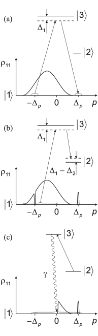
FIG. 1.: Energy level diagram and profile of ground state atomic distribution $\rho_{11}$ as a function of $p$, the momentum component along the direction of vector ${\bf{\Delta}}_{p}$: (a) before DS transfer with the two-photon $|1\rangle\to|1\rangle$ transition; (b) before the Raman excitation $|1\rangle\to|2\rangle$ cycle; and (c) before the optical repumping pulse tuned to the $|2\rangle\to|3\rangle$ transition. The curly braces denote momentum intervals involved in each of these processes.

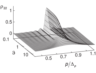
FIG. 2.: Velocity selectivity of Raman excitation in 1D case for Na represented as the dependence of $\rho_{22}$, the state $|2\rangle$ population, on the momentum component $p=p_{z}$ and parameter $\vartheta=Lf_{2}\tau_{0}/\hbar$. Detunings $\Delta_{1}=\Delta_{2}=-16\gamma$ and Rabi frequencies $\Omega_{1}=0.16\gamma$, $\Omega_{2}=0.016\gamma$.

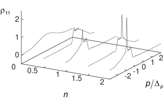
FIG. 3.: One-dimensional ground-state distribution $\rho_{11}$ for Na as a function of atomic momentum $p$ and the number $n$ of cooling cycles normalized to $1$ on the scale $p/\Delta_{p}$. Half-integer values of $n$ correspond to the beginning of the second stage of each cooling cycle which starts when laser beams reverse. The curve with $n=0$ gives the initial distribution. The highest peaks of the function represent the DS.

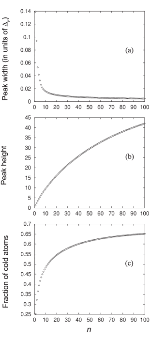
FIG. 4.: Parameters of the DS peak vs the number of cooling cycles. (a) Peak width at the half-maximum, (b) peak height, and (c) fraction of cold atoms around DS in the interval $\pm\delta p\approx\pm 0.14\Delta_{p}$, which spreads between the first minima in momentum dependence of the $|1\rangle\to|1\rangle$ transition rate.

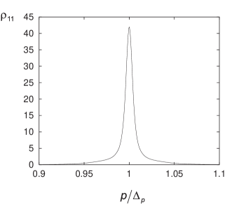
FIG. 5.: Final ground-state distribution $\rho_{11}$ of atoms with positive momenta as a function of $p$. The full-scale distribution is normalized as in the Fig. 3 whereas the plotted part contains $\sim 59\%$ of all particles.

REFERENCES

• [1] P. Lett, R. Watts, C. Westbrook, W. Phillips, P. Gould, and H. Metcalf, Phys. Rev. Lett. 61, 169 (1988).
• [2] A. Aspect, E. Arimondo, R. Kaiser, N. Vansteenkiste, and C. Cohen-Tannoudji, Phys. Rev. Lett. 61, 826 (1988); J. Lawall, S. Kulin, B. Saubamea, N. Bigelow, M. Leduc, and C. Cohen-Tannoudji, ibid. 75, 4194 (1995).
• [3] M. Kasevich and S. Chu, Phys. Rev. Lett. 69, 1741 (1992); N. Davidson, H. J. Lee, M. Kasevich, and S. Chu, ibid. 72, 3158 (1994); H. J. Lee, C. S. Adams, M. Kasevich, and S. Chu, ibid. 76, 2658 (1996).
• [4] R. Dum, Phys. Rev. A 54, 3299 (1996).
• [5] R. Dum and M. Ol’shanii, Phys. Rev. A 55, 1217 (1997).
• [6] T. Pellizzari, P. Marte, and P. Zoller, Phys. Rev. A 52, 4709 (1995).
• [7] G. Morigi, J. I. Cirac, K. Ellinger, and P. Zoller, Phys. Rev. A 57, 2209 (1998).
• [8] J. Reichel, F. Bardou, M. Ben Dahan, E. Peik, S. Rand, C. Salomon, and C. Cohen-Tannoudji, Phys. Rev. Lett. 75, 4575 (1995).
• [9] P. E. Moskowitz, P. L. Gould, S. R. Atlas, and D. E. Pritchard, Phys. Rev. Lett. 51, 370 (1983).
• [10] P. J. Martin, B. C. Oldaker, A. N. Miklich, and D. E. Pritchard, Phys. Rev. Lett. 60, 515 (1988).
• [11] A. V. Soroko, J. Phys. B. 30, 5621 (1997).
• [12] A. P. Kazantsev, G. A. Ryabenko, G. I. Surdutovich, and V. P. Yakovlev, Phys. Rep. 129, 75 (1985).
• [13] W. Zhang and D. F. Walls, Phys. Rev. A 52, 4696 (1995).
• [14] E. A. Korsunsky, D. V. Kosachiov, B. G. Matisov, and Yu. V. Rozhdestvensky, JETP 76, 210 (1993).
• [15] W. Zhang and D. F. Walls, Phys. Rev. A 49, 3799 (1994).
• [16] A. M. Guzman, M. Moore, and P. Meystre, Phys. Rev. A 53, 977 (1996).
• [17] V. Minogin and V. Letokhov, Laser Light Pressure on Atoms (Gordon and Breach, New York, 1986).
• [18] A. Aspect, E. Arimondo, R. Kaiser, N. Vansteenkiste, and C. Cohen-Tannoudji, J. Opt. Soc. Am. B 6, 2112 (1989).
• [19] B. Matisov, V. Gordienko, E. Korsunsky, and L. Windholz, JETP 80, 386 (1995).
• [20] E. A. Korsunsky, W. Maichen, and L. Windholz, Phys. Rev. A 56, 3908 (1997).
• [21] M. Lewenstein, L. You, J. Cooper, and K. Burnett, Phys. Rev. A 50, 2207 (1994).
• [22] R. J. C. Spreeuw, T. Pfau, U. Janicke, and M. Wilkens, Europhys. Lett. 32, 469 (1995); H. M. Wiseman and M. J. Collett, Phys. Lett. A 202, 246 (1995); M. Holland, K. Burnett, C. Gardiner, J. I. Cirac, and P. Zoller, Phys. Rev. A 54, R1757 (1996); G. M. Moy, J. J. Hope, and C. M. Savage, ibid. 55, 3631 (1997).
Refer to caption