Aharonov-Bohm scattering on a cone

M. Alvarez

Department of Physics,
University of Wales Swansea
Singleton Park, Swansea SA2 8PP, U.K.

e-mail: pyma@swansea.ac.uk

ABSTRACT

The Aharonov-Bohm scattering amplitude is calculated in the context of planar gravity with localized sources which also carry a magnetic flux. These sources cause space-time to develop conical singularities at their location, thus introducing novel effects in the scattering of electrically charged particles. The behaviour of the wave function in the proximity of the classical scattering directions is analyzed by means of an asymptotic expansion previously introduced by the author. It is found that, in contrast with the Aharonov-Bohm effect in flat space, integer values of the numerical flux can produce observable effects.
PACS: 03.65.Bz

SWAT-98-189 April 1998

physics/9804032

1 Introduction

The Aharonov-Bohm (-Ehrenberg-Siday) effect [1, 2] is a well-known example of quantum scattering process without classical analog, and its importance is reflected in the large number of analyses that have appeared in the literature (see the monograph [3] for a thorough exposition and a long list of references). The idealized experiment that produces the Aharonov-Bohm (AB) effect in its simplest version requires little description: charged particles of non-zero mass propagate at right angles to an infinitely long straight solenoid that encloses a magnetic flux; the region containing the magnetic field is inaccessible to the particles, in spite of which the magnetic flux inside the solenoid affects their propagation and an interference pattern appears that cannot be explained in classical physics. Among many references, [4, 5] are particularly relevant and readable. Detailed descriptions of real experimental set-ups can be found in [3] but we shall not be concerned with the practical aspects of the problem.

In this work we shall introduce a further complication in the problem: our flux tubes will have a non-vanishing mass density and will introduce gravitational effects in the motion of the scattered particles. In order to make the problem amenable we shall restrict ourselves to the simplest situation of an infinitely long and thin straight flux tube with constant magnetic flux and mass density. We shall sometimes call the idealized flux tube “string”. The advantage of the restriction just mentioned is that the gravitational field of the string can be described by general relativity in $2+1$ dimensions [6, 7], as the third spatial dimension can be taken to be parallel to the flux and will decouple from the problem. In the absence of other sources of gravity, the space created by the string will be locally flat everywhere except at the location of the string, and globally will be a $2$-cone. The time dimension remains unaffected as the string is taken to be static and at rest. The charged particle will be assumed to be massive but light enough to have negligible effect on the gravitational field of the string.

Given the previous simplifications, the object of interest is the wave function and scattering amplitude of a charged test particle moving in the conical background created by the flux line, hence the title of this paper. Naturally the solution will be a combination of planar gravitational scattering and AB scattering. The pure gravitational scattering amplitude was calculated in [6, 7, 8, 9] (see also [10]), and the pure AB scattering amplitude in [2, 11]-[18] following different procedures. The definition of the scattering amplitude requires knowledge of the long-distance behaviour of the scattered wave function, and usually the limit $r\to\infty$, with $r$ the distance from the scattering center, can be taken safely. One of the peculiarities of our problem is that, as in the purely gravitational case, there are two distinguished scattering directions independent of the energy of the incident particle that we call “classical” scattering directions, and the limits “approaching a classical scattering direction” and “$r\to\infty$” do not commute. If we take the long-distance limit first, the wave function develops singularities at the classical scattering directions, and if we approach those directions first then the long-distance limit does not exist. Physically the problem is that at the classical scattering directions the splitting of the wave function into “scattered” and “incident” (or transmitted) parts is no longer meaningful; only the complete wave function is free from discontinuities or singularities [9, 18]. The scattering amplitude, therefore, cannot be defined at those directions. This phenomenon occurs in the AB effect at the forward direction and in scattering in planar gravity at two directions that depend on the mass of the scattering center only [6, 7].

The analysis of the wave function near the classical scattering directions is best performed in the approach of [9] for planar gravitational scattering and [18] for AB scattering, and here the same approach will be used to solve the more general case of the AB effect on a cone. This article is organized as follows. In Section 2 we shall review the non-relativistic propagator of a charged particle in presence of a massive magnetic flux line. A piece of the propagator is given as an integral that is calculated in Section 3, where the result is used to obtain an asymptotic expansion of the propagator. We find that gravitational effects split the wave function into two halves that propagate along the classical scattering directions, and the two halves carry opposite AB-like phases. The last Section contains a discussion of the results; we conclude that, in contrast with the pure AB effect, the integer part of the numerical flux can be measured by means of an (imaginary) interference experiment.

2 The quantum-mechanical propagator

We are interested in the problem of a charged particle moving on a conical background created by a massive flux tube assumed to coincide with the $z$-axis. We recall that in this situation (quantum scattering of a test-particle by a static mass) the time-component of the metric does not play any role. A convenient characterization of this conical space is based on embedded coordinates [7]

$$(dl)^{2}=\alpha^{-2}(dr)^{2}+r^{2}(d\theta)^{2},\qquad\qquad-\pi\leq\theta\leq\pi,$$ (1)

where $0\leq(1-\alpha)=4MG<1$ and $G$ is “Newton’s constant”. If we consider that the incoming charged particles approach perpendicularly the flux line, the scattering process is essentially two-dimensional. In this situation a possible choice of vector potential is

$${\bf A}({\bf r})={\Phi\over 2\pi}\nabla\theta={c\hbar\over e}\nu\nabla\theta,$$ (2)

where $\Phi$ is the flux carried by the string, $\nu$ is the “numerical flux” defined as $\nu=e\Phi/2\pi\hbar c$ and $\theta$ is the polar angle of cylindrical coordinates described above. The Hamiltonian that defines the dynamics of the system is

$$H=-{\hbar^{2}\over 2m}\left({\bf p}-{e\over c}{\bf A}({\bf r})\right)^{i}g_{ij}\left({\bf p}-{e\over c}{\bf A}({\bf r})\right)^{j}$$

with ${\bf A}({\bf r})$ given by (2) and the metric $g_{ij}$ corresponding to the line element (1). Based on previous results [9, 18] we expect the wave function to exhibit two privileged scattering directions that depend only on the mass density of the flux line, and superimposed on each of these directions AB-like phases induced by the magnetic flux . As the separate cases of planar gravitational scattering and AB scattering are known, all we have to do is combine the propagators analyzed in the above mentioned references. The result can be given as a Bessel series [10]

$$G(r,\theta;r^{\prime},\theta^{\prime};\alpha;\nu;t)={m\over 2\pi\mathrm{i}\hbar t\alpha^{2}}\exp\left\{\mathrm{i}{m\over 2\hbar t\alpha^{2}}(r^{2}+r^{\prime 2})\right\}\sum_{n=-\infty}^{\infty}\mathrm{e}^{\mathrm{i}n(\theta-\theta^{\prime})}\,\mathrm{e}^{-\mathrm{i}{\pi\over 2\alpha}|\nu-n|}\,J_{{1\over\alpha}|\nu-n|}\left({mrr^{\prime}\over\hbar t\alpha^{2}}\right),$$

or, after inserting the Schläfli representation for the Bessel functions [13, 7, 8], as the sum of a “transmited” plus a “scattered” part, the last one being in integral form:

$$G_{\rm{tr}}(r,\theta;r^{\prime},\theta^{\prime};\alpha;\nu;t) = {m\over 2\pi\mathrm{i}\hbar t\alpha}\,\mathrm{e}^{\mathrm{i}\nu\phi}\mathop{{\sum}^{\prime}}_{n=-\infty}^{\infty}\exp\Big{\{}\mathrm{i}{m\over 2\hbar t\alpha^{2}}\big{[}r^{2}+r^{\prime 2}-2rr^{\prime}\cos\alpha(\theta-\theta^{\prime}+2\pi n)\big{]}\Big{\}}\,\mathrm{e}^{\mathrm{i}2\pi n\nu},$$

$$G_{\rm{sc}}(r,\theta;r^{\prime},\theta^{\prime};\alpha;\nu;t) = -{m\over 4\pi^{2}\hbar t\alpha^{2}}\exp\left\{\mathrm{i}{m\over 2\hbar t\alpha^{2}}(r^{2}+r^{\prime 2})\right\}\,\mathrm{e}^{\mathrm{i}[\nu]\phi}\int\limits_{-\infty}^{\infty}dy\,\exp\left\{\mathrm{i}{mrr^{\prime}\over\hbar t\alpha^{2}}\cosh y+{1\over\alpha}{{\{}\nu{\}}}y\right\}$$ (3)

$$\times\left[{\mathrm{e}^{-\mathrm{i}{{\{}\nu{\}}}{\pi\over\alpha}}\over 1-\mathrm{e}^{-\mathrm{i}(\theta-\theta^{\prime})+{1\over\alpha}(y-\mathrm{i}\pi)}}-{\mathrm{e}^{\mathrm{i}{{\{}\nu{\}}}{\pi\over\alpha}}\over 1-\mathrm{e}^{-\mathrm{i}(\theta-\theta^{\prime})+{1\over\alpha}(y+\mathrm{i}\pi)}}\right],$$

where the primed sum includes only $n$ such that $\alpha(\theta-\theta^{\prime}+2\pi n)\in(-\pi,\pi)$. The symbols $[\nu]$ and $\{\nu\}$ are the integer and fractional parts of the numerical flux $\nu$. The suffixes of the two parts of the propagator in (3) indicate that one part corresponds to the transmitted and the other to the scattered waves, although this splitting of the total propagator should not be taken literally because, as we shall see, both parts are required to determine the wave function of the “scattered” particle at the classical scattering directions. The propagator (3) reduces to the AB propagator if $\alpha=1$ and to the Deser-Jackiw propagator [7] of planar gravitational scattering if $\nu=0$. As in [9, 18] the propagator (3) leads to an integral than can be calculated by a saddle-point approximation for all scattered directions except the classical ones. The integral in question is

$$I(\rho,\phi,\alpha,\nu)=\int\limits_{-\infty}^{\infty}dy\,\exp\left\{\mathrm{i}\rho\cosh y+{1\over\alpha}{{\{}\nu{\}}}y\right\}\left[{\mathrm{e}^{-\mathrm{i}{{\{}\nu{\}}}{\pi\over\alpha}}\over 1-\mathrm{e}^{-\mathrm{i}\phi+{1\over\alpha}(y-\mathrm{i}\pi)}}-{\mathrm{e}^{\mathrm{i}{{\{}\nu{\}}}{\pi\over\alpha}}\over 1-\mathrm{e}^{-\mathrm{i}\phi+{1\over\alpha}(y+\mathrm{i}\pi)}}\right].$$ (4)

where we have defined the parameters $\rho$ and $\phi$ as

$$\rho = {mrr^{\prime}\over\hbar t\alpha^{2}},$$

$$\phi = \theta-\theta^{\prime}.$$

The saddle-point calculation of (4) requires the limit $\rho\to\infty$ to be taken in the exponential part of the integrand and then the integral is concentrated about $y\approx 0$ and is approximately Gaussian. This calculation has been done before [13, 7, 8] and does not need to be repeated here. We simply quote the resulting expression for the scattered propagator:

$$G_{\rm{sc}}(r,\theta;r^{\prime},\theta^{\prime};\alpha;\nu;t)\sim\mathrm{e}^{\mathrm{i}{3\over 4}\pi}\sqrt{m\over 8\pi^{3}\hbar t\alpha^{2}rr^{\prime}}\exp\left\{\mathrm{i}{m\over 2\hbar t\alpha^{2}}(r+r^{\prime})^{2}\right\}\mathrm{e}^{\mathrm{i}[\nu]\phi}{\mathrm{e}^{\mathrm{i}\phi}\sin{{{\{}\nu{\}}}\pi\over\alpha}+\sin({\pi\over\alpha}(1-{{\{}\nu{\}}}))\over\cos\phi-\cos{\pi\over\alpha}}.$$ (5)

We have used the notation $\sim$ to indicate that the equation is an asymptotic expansion for large $\rho$ [19]. From this result we can immediately write down the scattering amplitude of a well-localized wave packet approaching the string from $\theta^{\prime}=\pi$ and incident momentum $k$ (with the same result for plane-wave scattering):

$$f(k,\theta)\sim{1\over\sqrt{2\pi k}}\mathrm{e}^{\mathrm{i}[\nu]\theta}\mathrm{e}^{-\mathrm{i}{{\{}\nu{\}}}\pi}\,{\mathrm{e}^{\mathrm{i}\theta}\sin{{{\{}\nu{\}}}\pi\over\alpha}-\sin({\pi\over\alpha}(1-{{\{}\nu{\}}}))\over\cos\theta+\cos{\pi\over\alpha}}.$$ (6)

This scattering amplitude reduces to the AB or to the planar gravitational case in the appropriate limits. Naturally the global phases included in (6) are irrelevant if we are interested in the scattering cross section $\sigma=|f|^{2}$ only. Let us now remember that the classical scattering directions in our problem correspond, if the incident angle is $\theta^{\prime}=\pi$, to the following two values for the scattering angle $\theta$ [6, 7, 8]:

$$\theta_{\pm}=\pm\left({\pi\over\alpha}-\pi\right).$$

The fact that the scattering amplitude (6) diverges at these two directions is of course not due to any pathologies of the scattering process but rather to the fact that, around $\theta=\theta_{\pm}$, the saddle point approximation is not warranted. In the next section we shall follow the approach of [9, 18] to determine the wave function at the two directions $\theta_{\pm}$.

3 Asymptotic expansions

We will now develop an asymptotic expansion of the integral $I(\rho,\phi,\alpha,\nu)$ defined in (4) that, unlike a mere saddle-point approximation, be applicable when the scattering angle $\theta$ is close or equal to the classical scattering directions $\theta_{\pm}$. To that end we write the integral (4) as a sum of two terms

$$I(\rho,\phi,\alpha,\nu) = \mathrm{e}^{-\mathrm{i}{{\{}\nu{\}}}{\pi\over\alpha}}\int\limits_{-\infty}^{\infty}dy\,\exp\left\{\mathrm{i}\rho\cosh y+{1\over\alpha}{{\{}\nu{\}}}y\right\}{1\over 1-\mathrm{e}^{-\mathrm{i}\phi+{1\over\alpha}(y-\mathrm{i}\pi)}}$$

$$-\mathrm{e}^{\mathrm{i}{{\{}\nu{\}}}{\pi\over\alpha}}\int\limits_{-\infty}^{\infty}dy\,\exp\left\{\mathrm{i}\rho\cosh y+{1\over\alpha}{{\{}\nu{\}}}y\right\}{1\over 1-\mathrm{e}^{-\mathrm{i}\phi+{1\over\alpha}(y+\mathrm{i}\pi)}}$$

$$\equiv \mathrm{e}^{-\mathrm{i}{{\{}\nu{\}}}{\pi\over\alpha}}I_{1}(\rho,\phi,\alpha,\nu)-\mathrm{e}^{\mathrm{i}{{\{}\nu{\}}}{\pi\over\alpha}}I_{2}(\rho,\phi,\alpha,\nu),$$

and we can consider one of the two integrals, say $I_{1}$, and treat the other one by analogy. Following the lines proposed in [9, 18] the integral $I_{1}$ can be expanded as a hypergeometric series that, as we shall see, has a finite discontinuity at the classical scattering directions:

$$I_{1}(\rho,\phi,\alpha,\nu)\sim\mathrm{e}^{-\mathrm{i}{\pi\over 4}}\sqrt{2}\,\mathrm{e}^{\mathrm{i}\rho}\sum_{m=0}^{\infty}\rho^{{{1\over 2}}-m}\mathrm{i}^{m}A_{2m}(\phi+{\pi\over\alpha},{{\{}\nu{\}}},\alpha)\,\Gamma(m-{{1\over 2}})\,F_{2}(1,-m+{3\over 2},\mathrm{i}a(\alpha\phi)\rho),$$ (7)

where the coefficients $A_{2m}(\phi+{\pi\over\alpha},{{\{}\nu{\}}},\alpha)$ and $a(\alpha\phi)$ are defined by the following relations

$${\cos\eta(s)-\cos(\alpha\theta)\over 1-\mathrm{e}^{\mathrm{i}({\eta(s)\over\alpha}-\theta)}}{\mathrm{e}^{\mathrm{i}{{{\{}\nu{\}}}\over\alpha}\eta(s)}\over\cos{\eta(s)\over 2}} = \sum_{m=0}^{\infty}\mathrm{e}^{\mathrm{i}m{\pi\over 4}}A_{m}(\theta,{{\{}\nu{\}}},\alpha)s^{m},$$

$$\eta(s) = 2\arcsin\left(\mathrm{e}^{-\mathrm{i}{\pi\over 4}}{1\over\sqrt{2}}s\right),$$

$$a(\alpha\phi) = \mathrm{e}^{-\mathrm{i}\pi}(1+\cos(\alpha\phi)).$$

These calculations are rather lengthy, although straightforward, and can be reproduced after following the explanations given in [9, 18]. Using these results we can consider the limit $a(\alpha\phi)\rho\to\infty$, which corresponds to long distances from the scattering center away from the classical scattering directions $\theta_{\pm}$. Although the actual calculations are a good illustration of the use of our expansion (7), the final result coincides with (5) and (6) and therefore is of little relevance. The true interest of (7) is its good behaviour about $\theta=\theta_{\pm}$, where the total integral develops a finite discontinuity. If for example $\phi=-\pi/\alpha+\epsilon$ with $\epsilon$ a very small angle, we obtain

$$I(\rho,-{\pi\over\alpha}+\epsilon,\alpha,\nu)\sim-{\mathrm{sgn}}(\epsilon)\pi\alpha\,\mathrm{i}\,\mathrm{e}^{-\mathrm{i}{{\{}\nu{\}}}{\pi\over\alpha}}\mathrm{e}^{\mathrm{i}\rho}+\mathrm{e}^{\mathrm{i}{\pi\over 4}}\mathrm{e}^{\mathrm{i}\rho}\sqrt{{2\pi\over\rho}}\left[\mathrm{e}^{-\mathrm{i}{{\{}\nu{\}}}{\pi\over\alpha}}\left({{1\over 2}}-{{\{}\nu{\}}}\right)+{\mathrm{e}^{\mathrm{i}{{\{}\nu{\}}}{\pi\over\alpha}}\over\mathrm{e}^{\mathrm{i}{2\pi\over\alpha}}-1}\right]+\ldots$$

where the dots indicate subdominant terms in the large $\rho$ limit. The scattered part of the propagator is therefore

$$G_{\rm{sc}}(r,-{\pi\over\alpha}+\pi+\epsilon;r^{\prime},\pi;\alpha;\nu;t)={m\over 2\pi\mathrm{i}\hbar t\alpha^{2}}\exp\left\{\mathrm{i}{m\over 2\hbar t\alpha^{2}}(r+r^{\prime})^{2}\right\}\,\left(-{\mathrm{sgn}}(\epsilon)\right){{1\over 2}}\alpha\mathrm{e}^{-\mathrm{i}\nu{\pi\over\alpha}}+\ldots.$$

The transmited propagator can be easily calculated by means of its explicit expresion given in (3) with the following result:

$$G_{\rm{tr}}(r,-{\pi\over\alpha}+\pi+\epsilon;r^{\prime},\pi;\alpha;\nu;t)={m\over 2\pi\mathrm{i}\hbar t\alpha^{2}}\exp\left\{\mathrm{i}{m\over 2\hbar t\alpha^{2}}(r+r^{\prime})^{2}\right\}\,\left(1+{\mathrm{sgn}}(\epsilon)\right){{1\over 2}}\alpha\mathrm{e}^{-\mathrm{i}\nu{\pi\over\alpha}}+\ldots.$$

Both discontinuities cancel out in the complete propagator and thus the complete wave function is finite at $\phi=-\pi/\alpha$. A similar result obtains at the other classical scattering direction $\phi=\pi/\alpha$, with different sign in the phase $\nu\pi/\alpha$. Clearly the complete propagators so obtained represent linear propagation of wave packets along the classical scattering directions.

         

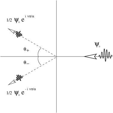
Figure 1: Aharonov-Bohm scattering of a wave packet on a cone

4 Interpretation and conclusions

The most interesting consequences of the propagators just obtained are that, at leading order in the long-distance limit, a wave packet approaching the magnetic tube will split into two halves that propagate along the classical scattering directions as in the case of pure gravitational scattering [9], and that the two halves carry opposite phases that depend on the combined parameter $\nu/\alpha$ only. The situation is schematically represented in Fig. 1, and agrees with the purely gravitational or AB cases in the appropriate limits.

The fact that the opposite phases of the two emerging wave packets depend on the whole numerical flux $\nu$ opens the possibility of measuring $\nu$ by means of an interference experiment. That imaginary experiment would consist in reuniting both diverging wave packets and allowing them to interfere on a flat screen perpendicular to the incident beam; the resulting interference pattern will show bands whose shift from the centered position depends on $\nu/\alpha$. As the parameter $\alpha$ can be measured from the scattering angle, $\nu$ can in principle be determined. This contrasts with the purely AB case, where only the fractional part of the flux can be measured.

Acknowledgements

This research has been supported by the Engineering and Physical Sciences Research Council (EPSRC) of the United Kingdom.

References

- [1] W. Ehrenberg, R. E. Siday, Proc. Phys. Soc. 62B, 8 (1949)
- [2] Y. Aharonov, D. Bohm, Phys. Rev. 115, 485 (1959)
- [3] M. Peshkin, A. Tonomura, The Aharonov-Bohm effect, Springer-Verlag Lecture Notes in Physics 340 1989
- [4] M. V. Berry, Eur. J. Phys. 1, 240 (1980)
- [5] M. V. Berry, Proc. R. Soc. Lond. A392, 45 (1984)
- [6] S. Deser, R. Jackiw, G. ’t Hooft, Ann. Phys. 152, 220 (1984)
- [7] S. Deser, R. Jackiw, Comm. Math. Phys. 118, 495 (1988)
- [8] R. Jackiw, P. de Sousa Gerbert, Comm. Math. Phys. 124, 229 (1989)
- [9] M. Alvarez, F. M. de Carvalho Filho, L. Griguolo, Comm. Math. Phys. 178, 467 (1996)
- [10] J. S. Dowker, J. Phys. A10 115 (1977)
- [11] M. V. Berry, R. G. Chambers, M. D. Large, C. Upstill, J. C. Walmsley, Eur. J. Phys. 1, 154 (1980)
- [12] T. Takabayashi, Hadronic Journal Supplement 1, 219, (1985)
- [13] R. Jackiw, Ann. Phys. 201, 83 (1990)
- [14] C. R. Hagen, Phys. Rev. D41, 2015 (1989)
- [15] A. Dasnières de Veigy, S. Ouvry, C. R. Acad. Sci. Paris t.318, Série II, 19 (1994)
- [16] S. N. M. Ruijsenaars, Ann. Phys. 146, 1 (1983)
- [17] D. Stelitano, Phys. Rev. D51, 5876 (1995)
- [18] M. Alvarez, Phys. Rev. A54 1128 (1996)
- [19] A. Erdélyi, Asymptotic Expansions, Dover Publications, New York, 1956; E. T. Copson, Asymptotic Expansions, Cambridge University Press, 1965.