On the Spinning Motion of the Hovering Magnetic Top.

Abstract

In this paper we analyze the spinning motion of the hovering magnetic top. We have observed that its motion looks different from that of a classical top. A classical top rotates about its own axis which precesses around a vertical fixed external axis. The hovering magnetic top, on the other hand, has its axis slightly tilted and moves rigidly as a whole about the vertical axis. We call this motion synchronous, because in a stroboscopic experiment we see that a point at the rim of the top moves synchronously with the top axis.

We show that the synchronous motion may be attributed to a small deviation of the magnetic moment from the symmetry axis of the top. We show that as a consequence, the minimum angular velocity required for stability is given by $\sqrt{4\mu HI_{1}/I_{3}^{2}}$ for $I_{3}>I_{1}$ and by $\sqrt{\mu H/(I_{3}-I_{1})}$ for $I_{3}<I_{1}$. Here, $I_{3}$ and $I_{1}$ are the principal and secondary moments of inertia, $\mu$ is the magnetic moment, and $H$ is the magnetic field. For comparison, the minimum angular for a classical top is given by $\sqrt{4\mu HI_{1}/I_{3}^{2}}$ both for $I_{3}<I_{1}$ and for $I_{3}>I_{1}$.

We also give experimental results that were taken with a top whose moment of inertia $I_{1}$ can be changed. These results show very good agreement with our calculations.

1 Introduction.

1.1 The hovering magnetic top.

The hovering magnetic top is an ingenious device that hovers in mid-air while spinning. It is marketed as a kit in the U.S.A. and Europe under the trade name Levitron^TM [1, 2] and in Japan under the trade name U-CAS[3]. The whole kit consists of three main parts: A magnetized top which weighs about 18gr, a thin (lifting) plastic plate and a magnetized square base plate (base). To operate the top one should set it spinning on the plastic plate that covers the base. The plastic plate is then raised slowly with the top until a point is reached in which the top leaves the plate and spins in mid-air above the base for about 2min. The hovering height of the top is approximately 3.0 cm above the surface of the base whose dimensions are about 10cm$\times$10cm$\times$2cm. The kit comes with extra brass and plastic fine tuning weights as the apparatus is very sensitive to the weight of the top. It also comes with two wedges to balance the base horizontally.

The hovering magnetic top serves as an excellent model to study many branches of physics. These include magnetism, electricity, hydrodynamics, mechanics of rigid body, wave mechanics, dynamical stability of non linear as well as linear systems, life time of quasi-stationary states and solid state magnetism to name just a few. For example, in the field of neutral particle trapping the hovering magnetic top is a vivid macroscopic device which demonstrates how it is possible to trap a neutral particle with spin in a static magnetic field. In fact, one of the recent examples of such traps was devised and applied to trap Rb⁸⁷ atoms and to form Bose-Einstein condensation[4, 5]. The trap used in this experiment is based on a rotating magnetic field and was given the name TOP (Time-averaged Orbiting Potential) trap. Though the TOP trap consists of a time dependent field it nevertheless operates on roughly the same principles as the trap of the hovering magnetic top. In addition to understanding magnetic traps there are many other issues that can be addressed by studying the hovering magnetic top. Questions such as: How high can it hover?, How long does it hover?, What are the tolerances on the mass of the top and the tilt angle of the base? How the trap works in the quantum regime? and other questions have been studied recently [6, 7, 8, 9, 10, 11] whereas other questions such as how does friction affect the stability of the top are currently under study.

1.2 The synchronous motion.

The physical principles underlying the dynamical stability of the hovering magnetic top rely on the so-called ‘adiabatic approximation’ and have recently been discussed in several papers [12, 13, 14, 15]. In these articles the top was modeled as an axially symmetric shape with its magnetization taken as a dipole pointing along the symmetry axis and situated at the center of mass. Observing the top as it hovers forced us however, to augment this picture by assuming that the dipole is canted by a small angle $\Delta$ with respect to the symmetry axis of the top. We were motivated by the fact that the motion of the magnetic top as it hovers looked different from that of a classical top (but also by recalling that it would be forced by manufacturing tolerances). As a classical top slows down it starts to deviate from the vertical while it precesses with a frequency which is not synchronous to the frequency of the spin of the top around its axis. The axis of the hovering magnetic top is also canted to the vertical but the motion is synchronous. There is only one frequency involved. This can even be seen with the naked eye. The axis of the magnetic top rotates around the vertical but synchronously with the spin of the top around itself. An analogy, though not literal, is helpful here: The motion of the hovering magnetic top is reminiscent of the motion of the moon around the earth but that of a classical top is more like the rotation of the earth around the sun. The astute observer watching the hovering magnetic top will note that the canting increases as the top slows down, even with the naked eye. It was more conspicuous to us when we observed it with a stroboscope preferably strobed at twice or three times the synchronous frequency. Using the latter frequency enabled also to measure the phase of the tilt. It is this way that we found this phase is correlated to the phase of $\Delta$- the canting of the magnetic moment with respect to the axis of the top. We reach the same conclusion by observing in slow motion videos of hovering tops in which we changed $\Delta$ artificially. As will be shown in the following the canting $\Delta$ explains all the above observations.

The present paper is in fact a study of the effect of this small canting $\Delta$ on the hovering of the magnetic top. In addition to explaining the above qualitative features we also derive quantitative results. In particular we show that the minimum angular velocity required for stability $\omega_{min}$ is given by

$$\omega_{min}=\left\{\begin{array}[]{ll}\sqrt{{\displaystyle{4\mu HI_{1}\over I_{3}^{2}}}}&\mbox{ for }I_{3}<I_{1}\\ \sqrt{{\displaystyle{\mu H\over I_{3}-I_{1}}}}&\mbox{ for }I_{3}>I_{1}.\end{array}\right.$$

Here, $I_{3}$ and $I_{1}$ are the principal and secondary moment of inertia, $\mu$ is the magnetic moment of the top and $H$ is the magnetic field. This result is to be contrasted with the minimum speed of a classical top[16] which is given by $\sqrt{4\mu HI_{1}/I_{3}^{2}}$ for both $I_{3}<I_{1}$ and $I_{3}>I_{1}$.

On the experimental side, we have measured the minimum speed of a hovering top whose moment of inertia $I_{1}$ can be changed so as to cover values both below and above $I_{3}$. These results show excellent agreement with our calculations.

1.3 The structure of this paper.

The structure of this paper is as follows: In Sec.(2) we carry out a detailed analysis of the synchronous motion. We first describe precisely what is meant by the synchronous motion and define our notations in Sec.(2.1). In Sec.(2.2) we study the conditions that must be met in order for the system to reach equilibrium. Next, in Sec.(2.3) we carry out a dynamical stability analysis to find under what conditions the equilibrium solution found previously is indeed stable. Finally, in Sec.(2.4) we combine all the conditions that were found both from equilibrium considerations and dynamical stability considerations, and arrive at the expressions for the minimum angular velocity. The description of our experiment and a comparison of the results with the theoretical calculations from the previous section is given in Sec.(3). In Sec.(4), we summarize our results and discuss possible extensions of the calculations presented in this paper and other related subjects.

2 Analysis of the Synchronous motion.

2.1 Description of the Problem.

As the top hovers above the magnetized plate, the magnetic lift force exerted by the base is balanced by the top weight. Therefore, to simplify further calculations we assume that gravity is zero and the magnetic field is homogeneous. Further, we disregard the translational motion of the top and assume that it move around a fixed point. This point is taken as the common origin of the moving and fixed system of coordinates. With these simplifications the synchronous motion can be modeled as shown in Fig.(1).

Figure 1: The synchronous motion: The top revolves rigidly around the vertical $\hat{\boldsymbol{z}}$ axis with angular velocity $\omega$. The principal axis of the top (axis $\hat{\boldsymbol{n}}$) makes an angle $\theta_{0}$ with the vertical. The whole system is in a uniform magnetic field, $H$, pointing downward. The top possesses a magnetic moment dipole, $\mu$, that makes an angle $\Delta$ with its principal axis.

The figure describes a top that rotates rigidly around the vertical $\hat{\boldsymbol{z}}$ axis with angular velocity $\omega$. The principal axis of the top (axis $\hat{\boldsymbol{n}}$) makes an angle $\theta_{0}$ with the vertical axis. The whole system is in a uniform magnetic field $H$, pointing downward. The top possesses a magnetic moment dipole, $\mu$, that makes an angle $\Delta$ with its principal axis.

2.2 Equilibrium considerations.

We first determine the angle between the top axis $\hat{\boldsymbol{n}}$ and the vertical axis $\hat{\boldsymbol{z}}$ from torque equilibrium. The angular momentum of a symmetric top has the form[17]

$$\boldsymbol{L}=I_{3}\omega_{3}\hat{\boldsymbol{n}}+I_{1}\hat{\boldsymbol{n}}\times{\displaystyle{d\hat{\boldsymbol{n}}\over dt}}$$ (1)

where $\omega_{3}$ is the component of the vector angular velocity $\hat{\omega}$ in the direction of the $\hat{\boldsymbol{n}}$ axis. Since $\hat{\boldsymbol{n}}$ is fixed in the body,

$${\displaystyle{d\hat{\boldsymbol{n}}\over dt}}=\mbox{\boldmath$\omega$}\times\hat{\boldsymbol{n}},$$ (2)

and therefore

$$\boldsymbol{L}=\left(I_{3}-I_{1}\right)\omega_{3}\hat{\boldsymbol{n}}+I_{1}\mbox{\boldmath$\omega$}.$$ (3)

For the synchronous motion, the gyroscopic torque in the co-moving frame must compensate the magnetic torque, hence

$$\mbox{\boldmath$\omega$}\times\boldsymbol{L}=\mbox{\boldmath$\mu$}\times\boldsymbol{H}.$$ (4)

Thus, $\mu$ has to be coplanar with $\hat{\boldsymbol{z}}$ and $\hat{\boldsymbol{n}}$, and one obtain, with $\omega_{3}=\omega\cos\theta_{0}$, the equilibrium condition

$$(I_{3}-I_{1})\omega^{2}\sin\theta_{0}\cos\theta_{0}=\mu H\sin(\theta_{0}+\Delta).$$ (5)

We assume that the angle $\Delta$ is small. Then, during its motion the top axis $\hat{\boldsymbol{n}}$ stays close to the $\hat{\boldsymbol{z}}$ axis, and we may use small angle approximation in Eq.(5) and express $\theta_{0}$ in terms of $\omega$ as follows:

$$\theta_{0}\simeq\frac{\mu H\Delta}{(I_{3}-I_{1})\omega^{2}-\mu H}.$$ (6)

In order to understand what Eq.(6) means we must resort to a more realistic description of the hovering top. If we take into account air friction and the inhomogeneity of the magnetic field, the following picture emerges: As the top hovers, it experience air friction which causes $\omega$ to decrease with time. Thus, according to Eq.(6) $\theta_{0}$ increases provided that $I_{3}>I_{1}$ (a disk-like top). This, on the other hand, decreases the repulsive force on the top which is caused by the field gradient. Thus, the top rebalances itself at a lower height. This process continues until the field gradient reaches its maximum value, that occurs at a height equal roughly to half the size of the base. At this point the magnetic field can no longer support the top and the latter falls down vertically. In our experiments we could clearly see that $\theta_{0}$ increases gradually by the naked eye. We conclude that when $\theta_{0}$ is ‘large enough’ the top will fall down. We denote by $\theta_{0}^{*}$ the maximum allowed angle. The angular velocity which correspond to this angle is, according to Eq.(6), given by

$$\omega=\sqrt{{\displaystyle{\mu H\left({\displaystyle{\Delta\over\theta_{0}^{*}}}+1\right)\over I_{3}-I_{1}}}}.$$ (7)

To estimate $\theta_{0}^{*}$ we recall that the tolernace on the weight is equal to the toleance allowed on the lift. It follows that[10]

$${\displaystyle{dm\over m}}\sim\frac{\left(\theta_{0}^{*}\right)^{2}}{2}.$$

Since the tolerance on the weight is about $2\%$ (see Ref.[10]) it follows that $\theta_{0}^{*}\sim 0.1$rad. Although we did not measure $\Delta$ directly, our experiments, including those in which we have artificially changed $\Delta$ indicate that $\Delta/\theta_{0}^{*}\ll 1$. It is therefore justified to neglect this term in Eq.(7) and we arrive to an approximate expression for the minimum speed when $I_{3}>I_{1}$, namely:

$$\omega_{min}^{stat}\simeq\sqrt{{\displaystyle{\mu H\over I_{3}-I_{1}}}}\mbox{ for }I_{3}>I_{1}.$$

For a rod-like top ($I_{3}<I_{1}$) the synchronous motion is also possible, but now $\Delta$ must be more negative than $-\theta_{0}$. This is because in this case the direction of the centrifugal torque is reversed, and for equilibrium to exist the magnetic torque must also be reversed. The condition that $\Delta<-\theta_{0}$ gives $\omega>0$ which signifies that as far as the equilibrium condition is concerned there is no minimum speed for this case. Following similar arguments as before it can be easily deduced that in this case $\theta_{0}$ decreases with time and the top slowly gains height as it slows down due to air friction. This is opposite of what we have found for a disk-like top.

Note also that the rod-like top exhibits diamagneic-like behavior. Namely, the differential susceptibility is in this case negative as can be seen from Eq.(6).

Summarizing our results so far we conclude that as far as the equilibrium condition is concerned the minimum allowed angular velocity depends on the eccentricity of the top and is given by

$$\omega_{min}^{stat}=\left\{\begin{array}[]{cc}\sqrt{{\displaystyle{\mu H\over I_{3}-I_{1}}}}&\mbox{ for a disk-like top }(I_{3}>I_{1})\\ 0&\mbox{ for a rod-like top }(I_{3}<I_{1})\mbox{,}\end{array}\right.$$ (8)

and is valid both for clockwise and counter-clockwise directions of the spin. Note that Eq.(8) is not the all answer because the dynamical stability should also be considered. This is done in the following section.

2.3 Dynamic stability considerations.

2.3.1 Overview

Up to this point we have studied conditions that were derived directly from the equilibrium condition. In this section we study the conditions that must be met in order to sustain the synchronous motion. We start by reformulating the equations of motion in terms of the Lagrangian formalism and Euler’s angles, and then add to the synchronous motion a small perturbation. We then arrive at a set of equations for the perturbational part and find the conditions that are required for the perturbation to be oscillatory which is the condition that the unperturbed motion is stable.

2.3.2 The Lagrangian and the equations of motion.

We denote the coordinate system fixed in space by $(\hat{\boldsymbol{x}},\hat{\boldsymbol{y}},\hat{\boldsymbol{z}})$ and the other that is fixed in the body by $(\hat{1},\hat{2},\hat{\boldsymbol{n}})$, as depicted in Fig.(2).

Figure 2: Definition of Euler’s angles.

The magnetic moment $\mu$ makes an angle $\Delta$ with the $\hat{\boldsymbol{n}}$ axis and lies in the $\hat{2}$-$\hat{\boldsymbol{n}}$ plane. Thus

$$\mbox{\boldmath$\mu$ }=\mu\left(\hat{\boldsymbol{n}}\cos\Delta-\hat{2}\sin\Delta\right).$$

The magnetic field is uniform and points along the $-\hat{\boldsymbol{z}}$ direction, i.e.

$$\boldsymbol{H}=-H\hat{\boldsymbol{z}}=-H\left(\hat{1}\sin\psi\sin\theta+\hat{2}\cos\psi\sin\theta+\hat{\boldsymbol{n}}\cos\theta\right),$$

where $\phi$, $\theta$ and $\psi$ are the first, second and third Euler’s angles, defined in Fig.(2). Therefore, the magnetic energy for this configuration has the form

$$E_{mag}=-\mbox{\boldmath$\mu$}\cdot\boldsymbol{H}=\mu H\left(\cos\theta\cos\Delta-\sin\Delta\cos\psi\sin\theta\right).$$

The kinetic energy, expressed using Euler’s angle, is

$$E_{kin}={\displaystyle{1\over 2}}I_{3}\left(\dot{\psi}+\dot{\phi}\cos\theta\right)^{2}+\frac{1}{2}I_{1}\left(\dot{\theta}^{2}+\dot{\phi}^{2}\sin^{2}\theta\right).$$

The Lagrangian $L$ is given by the difference between the kinetic energy $E_{kin}$ and the magnetic energy $E_{mag}$,

$$\begin{array}[]{c}L={\displaystyle{1\over 2}}I_{3}\left(\dot{\psi}+\dot{\phi}\cos\theta\right)^{2}+{\displaystyle{1\over 2}}I_{1}\left(\dot{\theta}^{2}+\dot{\phi}^{2}\sin^{2}\theta\right)\\ -\mu H\left(\cos\theta\cos\Delta-\sin\Delta\cos\psi\sin\theta\right).\end{array}$$ (9)

The dynamics of motion for this system is then governed by the Lagrange equations of motion

$$\begin{array}[]{c}{\displaystyle{d\over dt}}\left({\displaystyle{\partial L\over\partial\dot{\theta}}}\right)-{\displaystyle{\partial L\over\partial\theta}}=0\\ {\displaystyle{d\over dt}}\left({\displaystyle{\partial L\over\partial\dot{\psi}}}\right)-{\displaystyle{\partial L\over\partial\psi}}=0\\ {\displaystyle{d\over dt}}\left({\displaystyle{\partial L\over\partial\dot{\phi}}}\right)-{\displaystyle{\partial L\over\partial\phi}}=0.\end{array}$$ (10)

With the Lagrangian given in Eq.(9) one obtains

$$\begin{array}[]{c}I_{1}\ddot{\theta}+\left[(I_{3}-I_{1})\dot{\phi}\cos\theta+I_{3}\dot{\psi}\right]\dot{\phi}\sin\theta=\mu H\left(\sin\theta\cos\Delta+\sin\Delta\cos\psi\cos\theta\right)\\ I_{3}\dot{\phi}\dot{\theta}\sin\theta-I_{3}\left(\ddot{\psi}+\ddot{\phi}\cos\theta\right)=\mu H\sin\Delta\sin\psi\sin\theta\\ \left(I_{3}\cos^{2}\theta+I_{1}\sin^{2}\theta\right)\dot{\phi}+I_{3}\dot{\psi}\cos\theta=L_{z}=\text{Const.}\end{array}$$ (11)

2.3.3 The Stationary Solution.

A stationary solution to the set Eqs.(11) is found by setting

$$\theta(t) = \theta_{0}=\text{Const.}$$ (12)

$$\psi(t) = \psi_{0}=\mbox{Const.}$$

Substituting these into the third equation of the set Eqs.(11) and integrating over time yields

$$\phi(t)=\omega=\mbox{Const.}$$ (13)

Using the second equation we find that

$$\psi_{0}=0,$$ (14)

while the remaining (first) equation gives

$$(I_{3}-I_{1})\omega^{2}\sin\theta_{0}\cos\theta_{0}=\mu H\sin(\theta_{0}+\Delta).$$ (15)

Note that Eq.(15) is identical to Eq.(5), which was derived in Sec.(2.2).

2.3.4 Perturbing the stationary solution.

We now perturb the stationary solution by adding small variations,

$$\begin{array}[]{c}\dot{\phi}(t)=\dot{\phi}_{s}(t)+\delta\dot{\phi}(t)=\omega+\delta\dot{\phi}(t)\\ \psi(t)=\psi_{s}(t)+\delta\psi(t)=0+\delta\psi(t)\\ \theta(t)=\theta_{s}(t)+\delta\theta(t)=\theta_{0}+\delta\theta(t)\end{array}$$ (16)

Substituting this these into Eqs.(11) and keeping only first-order terms yields

$$\begin{array}[]{c}\begin{array}[]{c}I_{1}\delta\ddot{\theta}+(I_{3}-I_{1})\omega\delta\dot{\phi}\sin(2\theta_{0})\\ +(I_{3}-I_{1})\omega^{2}\delta\theta\cos(2\theta_{0})+I_{3}\delta\dot{\psi}\omega\sin\theta_{0}=\mu H\delta\theta\cos(\Delta+\theta_{0})\end{array}\\ I_{3}(\delta\ddot{\psi}+\delta\ddot{\phi}\cos\theta_{0})-I_{3}\delta\dot{\theta}\omega\sin\theta_{0}+\mu H\sin\Delta\delta\psi\sin\theta_{0}=0\\ \begin{array}[]{c}-2\omega(I_{3}-I_{1})\delta\theta\sin\theta_{0}\cos\theta_{0}+I_{3}\delta\dot{\psi}\cos\theta_{0}\\ +\delta\dot{\phi}\left(I_{3}\cos^{2}\theta_{0}+I_{1}\sin^{2}\theta_{0}\right)=0\end{array}.\end{array}$$ (17)

Using Eq.(15) we express $\Delta$ in terms of $\theta_{0}$ and to simplify further calculations we now restrict ourselves to the case where $\theta_{0}$ is a small angle and work to second-order in $\theta_{0}$. Under the small-angle approximation Eqs.(17) becomes

$$\begin{array}[]{c}\begin{array}[]{c}I_{1}\delta\ddot{\theta}+2(I_{3}-I_{1})\omega\delta\dot{\phi}\theta_{0}+(I_{3}-I_{1})\omega^{2}\delta\theta\left(1-2\theta_{0}^{2}\right)\\ +I_{3}\delta\dot{\psi}\omega\theta_{0}=\mu H\delta\theta\left(1-0.5\beta^{2}\theta_{0}^{2}\right)\end{array}\\ \begin{array}[]{c}I_{3}\delta\ddot{\psi}+I_{3}\delta\ddot{\phi}\left(1-{\displaystyle{1\over 2}}\theta_{0}^{2}\right)-I_{3}\delta\dot{\theta}\omega\theta_{0}\\ +(\omega^{2}(I_{3}-I_{1})-\mu H)\theta_{0}^{2}\delta\psi=0\end{array}\\ \begin{array}[]{c}-2\omega\theta_{0}(I_{3}-I_{1})\delta\dot{\theta}+I_{3}\delta\ddot{\psi}\left(1-\frac{1}{2}\theta_{0}^{2}\right)\\ +I_{3}\delta\ddot{\phi}\left(1-\theta_{0}^{2}\right)+I_{1}\delta\ddot{\phi}\theta_{0}^{2}=0.\end{array}\end{array}$$ (18)

where $\beta=\left(I_{3}-I_{1}\right)\omega^{2}/\mu H-2$.

Since Eqs.(18) are linear in the perturbations and homogenous, the general solution of these equations is a linear combination of exponential functions. We therefore set

$$\begin{array}[]{c}\delta\theta(t)=\delta\theta_{0}e^{\lambda t}\\ \delta\phi(t)=\delta\phi_{0}e^{\lambda t}\\ \delta\psi(t)=\delta\psi_{0}e^{\lambda t}\end{array}$$

and substitute these into Eqs.(18). The result is the matrix equation for the determination of the eigenvalues $\lambda$

$$\boldsymbol{A}\left[\begin{array}[]{c}\delta\theta_{0}\\ \delta\phi_{0}\\ \delta\psi_{0}\end{array}\right]=\left[\begin{array}[]{c}0\\ 0\\ 0\end{array}\right],$$

where $\boldsymbol{A}$ is the matrix given by:

$$\left[\begin{array}[]{ccc}\left(\begin{array}[]{c}\lambda^{2}I_{1}-\mu H(1-0.5\beta^{2}\theta_{0}^{2})\\ +(I_{3}-I_{1})\omega^{2}(1-2\theta_{0}^{2})\end{array}\right)&2\lambda(I_{3}-I_{1})\omega\theta_{0}&\lambda I_{3}\omega\theta_{0}\\ -\lambda I_{3}\omega\theta_{0}&\lambda^{2}I_{3}(1-{\displaystyle{1\over 2}}\theta_{0}^{2})&\left(\begin{array}[]{c}\lambda^{2}I_{3}\\ +\left[\omega^{2}\left(I_{3}-I_{1}\right)-\mu H\right]\theta_{0}^{2}\end{array}\right)\\ -2\omega\lambda(I_{3}-I_{1})\theta_{0}&\left(\begin{array}[]{c}\lambda^{2}I_{3}(1-\theta_{0}^{2})\\ +\lambda^{2}I_{1}\theta_{0}^{2}\end{array}\right)&\lambda^{2}I_{3}(1-\frac{1}{2}\theta_{0}^{2})\end{array}\right]$$ (19)

For a nontrivial solution to exist, the determinant of the matrix must vanish. After a few algebraic steps we find

$$\det\boldsymbol{A}=-\lambda^{2}I_{3}\theta_{0}^{2}\left(a\lambda^{4}+b\lambda^{2}+c\right)+{\cal O}\left(\theta_{0}^{4}\right)=0,$$

where

$$a \equiv I_{1}^{2}$$

$$b \equiv -2I_{1}\left[\mu H-\omega^{2}(I_{3}-I_{1})\right]-\omega^{2}(I_{3}-2I_{1})(2I_{1}-I_{3})$$

$$c \equiv \left[\mu H-\omega^{2}(I_{3}-I_{1})\right]^{2}$$

Thus, we find a doubly degenerate zero eigenvalue corresponding to the cyclic coordinate $\phi$, which enter the equations of motion only through its time derivative. The other eigenvalues are the roots of a quadratic equation in $\lambda^{2}$.

For the perturbation to be bounded for all times, the non-vanishing eigenvalues must be purely imaginary. Thus, the two $\lambda^{2}$ roots must be both real and negative. The condition for these roots to be real is that $b^{2}-4ac>0$. This results in the inequality

$${\displaystyle{\mu H\over\omega^{2}I_{1}}}<\frac{1}{4}\left({\displaystyle{I_{3}\over I_{1}}}\right)^{2},$$ (20)

which is the well-known stability condition of a classical top with one point fixed[16]. For both roots to be negative, their product must be positive (i.e. $c/a>0$) and their sum must be negative ($-b/a<0$). Since both $a$ and $c$ are squares of real numbers, their ratio is positive. We thus find as the second condition

$${\displaystyle{\mu H\over\omega^{2}I_{1}}}<{\displaystyle{1\over 2}}\left({\displaystyle{I_{3}\over I_{1}}}\right)^{2}-\left({\displaystyle{I_{3}\over I_{1}}}\right)+1.$$ (21)

It may be easily verified that for a physical top, for which $I_{3}<2I_{1}$, the inequality Eq.(21) is satisfied whenever Eq.(20) holds. Therefore, the overall condition for the stability of the synchronous motion is given by Eq.(20) alone, namely

$$\omega_{min}^{dyn}=\sqrt{{\displaystyle{4\mu HI_{1}\over I_{3}^{2}}}}$$ (22)

both for $I_{3}>I_{1}$ and for $I_{3}<I_{1}$.

2.4 Conclusions.

Hitherto we have found separate conditions for the minimum angular speed, one pair given in Eq.(8) arising from equilibrium considerations, the other one given in Eq.(22) originating from dynamical stability considerations. Since these conditions must be satisfied simultaneously, we now take the union of these conditions. Taking into account the fact that for a disk-like top $\sqrt{\mu H/(I_{3}-I_{1})}$ is larger than $\sqrt{4\mu HI_{1}/I_{3}^{2}}$, we find that the union of these conditions amounts to the following expressions for $\omega_{min}$:

$$\omega_{min}=\left\{\begin{array}[]{cc}\sqrt{{\displaystyle{\mu H\over I_{3}-I_{1}}}}&\mbox{ for a disk-like top }(I_{3}>I_{1})\\ \sqrt{{\displaystyle{4\mu HI_{1}\over I_{3}^{2}}}}&\mbox{ for a rod-like top }(I_{3}<I_{1}).\end{array}\right.$$ (23)

According to this result, there should be an abrupt change in $\omega_{min}$ in the vicinity of a sphere-like top ($I_{1}=I_{3}$) even for a vanishingly small value of the angle $\Delta$. This abrupt change is also found in our experiments, as is shown in the next section.

3 Experimental Results.

To test our calculations we have built a magnetized top whose moment of inertia $I_{1}$ can be changed so as to cover values both below and above $I_{3}$. We have measured the minimum angular speed of the top for several values of $I_{1}/I_{3}$. Fig.(3) shows (in bullets) the reciprocal of the measured angular speed normalized to the minimum angular speed of a pure disk top versus $x\equiv(I_{3}-I_{1})/I_{1}$. To compare these results to our calculation we rewrite Eq.(23) as an equation for the normalized reciprocal angular speed $\omega_{min}\left(1\right)/\omega_{min}\left(x\right)$ in terms of $x$. The result is

$${\displaystyle{\omega_{min}\left(1\right)\over\omega_{min}\left(x\right)}}=\left\{\begin{array}[]{cc}\sqrt{{\displaystyle{2x\over x+1}}}&;\mbox{ }0<x<1\\ \sqrt{{\displaystyle{x+1\over 2}}}&\mbox{ };-1<x<0.\end{array}\right.$$

Fig.(3) shows $\omega_{min}\left(1\right)/\omega_{min}\left(x\right)$ as a solid line. It is clear from the figure that the experimental results support our theory.

The two main features of our theoretical results are: 1) the divergence of $\omega_{min}$ for disk-like tops as they approach spherical shape and 2) the discontinuity in $\omega_{min}$ as one goes over to rod-like top. 1) Unfortunately, we could not go beyond $\omega>2.5\omega_{min}(1)$ because the maximum spin frequency is limited by the dynamic stability of the top in the trap[14]. It is therefore impossible to observe experimentally the above divergence. 2) Though we have only two measured points at the rod-like part of the graph it is conspicuous that they verify the difference in the origin of the instability for disk- and rod-like tops that our theory shows.

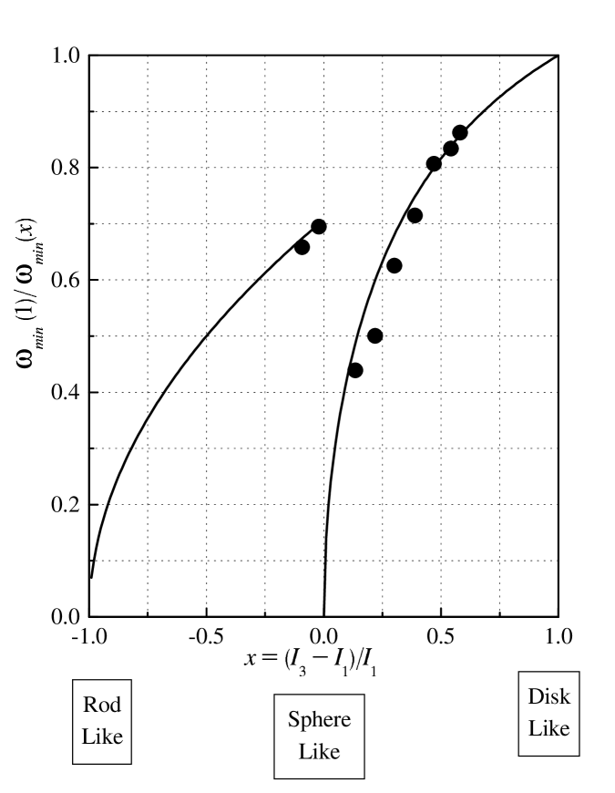
Figure 3: Reciprocal of the normalized minimum angular velocity versus top shape. The bullets are the measured results and the solid line is the calculated results.

4 Discussion.

In this paper we have analyzed one possible cause for the synchronous motion and attributed it to the small difference between the direction of the principal axis of inertia and the direction of the magnetic moment. We have shown that as a consequence, for a disk-like top the minimum angular velocity required for stability differs from that for a classical top (with one point fixed) and is given by:

$$\omega_{min}=\left\{\begin{array}[]{ll}\sqrt{{\displaystyle{4\mu HI_{1}\over I_{3}^{2}}}}&\mbox{ for }I_{3}<I_{1}\\ \sqrt{{\displaystyle{\mu H\over I_{3}-I_{1}}}}&\mbox{ for }I_{3}>I_{1}\end{array}\right.$$

where $I_{3}$ and $I_{1}$ are the principal and secondary moment of inertia, $\mu$ is the magnetic moment of the top and $H$ is the magnetic field. This result is found to be in a very good agreement with our experiments.

We remark that in the calculations presented in this paper we have neglected some aspects which are relevant to the behavior of the top. For example, the dipole moment of the top carries with it a minute amount of intrinsic spin of the order of $S\sim\hbar\mu/\mu_{B}$ where $\hbar$ is Planck’s constant and $\mu_{B}$ is the Bohr’s magneton. The existence of the spin contributes an additional term to the total angular momentum written in Eq.(2). In this case the symmetry between clockwise (CW) and counter-clockwise (CCW) rotations breaks down, and one finds different values for the minimum angular speed for each direction. Due to the smallness of the spin with respect to the orbital angular momentum, the CW-CCW asymmetry becomes pronounced only when the size of the top is of the order of tenths of microns. Our calculations show that when the sense of rotation is roughly antiparallel to the direction of the spin the minimum angular speed increases, whereas when it is roughly parallel to the spin, the minimum angular speed decreases. This conclusion immediately raises the question whether it is possible to hover a top using its intrinsic spin alone without the need to spin it. To study this we assume the top to be endowed intrincily with spin proportional to its magnetic moment. We find that it may be possible to hover a top having only this spin with no additional angular momentum[18].

Another interesting point is what happens if we relinquish the requirement that $\theta_{0}$ is small. Note that the equilibrium equation Eq.(5) is that of the well-known Stoner and Wolfarth model (SW)[19, 20], extensively used to described the hysteresis of single domain ferromagnetic particles. In that case at most only two of the equilibria are stable. We find, however, in our case the unstable SW becomes stable under some conditions, being stabilized by the dynamics. A word of warning is due here when applying these results to the hovering top. We have in this work considered only the rotational degrees of freedom, and what is stable under these is not necessarily stable any more in an inhomogeneous field necessary to trap the top. We believe however that the small angle solution is still stable there under the same conditions that are given by us[14] for $\Delta=0$.

References

- [1] The Levitron is available from ‘Fascinations’, 18964 Des Moines Way South, Seattle, WA 98148.
- [2] Hones et al., U.S. Patent Number: 5,404,062, Date of Patent: Apr. 4, 1995.
- [3] The U-CAS is available from Masudaya International Inc., 6-4, Kuramae, 2-Chome, Taito-Ku, Tokyo, 111 Japan.
- [4] ‘Physics Today’, Aug. 1995, pp. 17-20.
- [5] W. Petrich, M. H. Anderson, J. R. Ensher and E. A. Cornell, Phys. Rev. Lett. , 17, 3352-3355 (1995).
- [6] S. Gov, S. Shtrikman and S. Tozik, Ann. Meet. of the IPS, , 122 (1996).
- [7] S. Gov, H. Matzner and S. Shtrikman, Ann. Meet. of the IPS, , 121 (1996).
- [8] S. Gov and S. Shtrikman, Proc. of the 19th Israel IEEE Conv., 184 (1996).
- [9] S. Gov, H. Matzner and S. Shtrikman, Proc. of the 19th Israel IEEE Conv., 121 (1996).
- [10] S. Gov, H. Matzner and S. Shtrikman, Ann. Meet. of the IPS, , 47 (1997).
- [11] S. Gov, S. Shtrikman and H. Thomas, Bulletin of the Israel Physical Society, , 81 (1998).
- [12] M. V. Berry, Proc. R. Soc. Lond. A, , 1207 (1996).
- [13] M. D. Simon, L. O. Heflinger and S. L. Ridgway, Am. J. Phys. , (4), 286 (1997).
- [14] S. Gov, S. Shtrikman and H. Thomas, Los-Alamos E-Print Archive, http://xxx.lanl.gov/, physics/9803020 (1998).
- [15] M. V. Berry, A. K. Geim, IOP Publishing Ltd and The European Physical Society, 307 (1997).
- [16] “Mechanics” by L. D. Landau and E. M. Lifshitz, Pergamon Press, 3rd Ed., 111-114.
- [17] “Vectorial Mechanics” by E. A. Milne, Methuen and Co. London, 322-323 (1948).
- [18] S. Gov, S. Shtrikman and H. Thomas, to be published.
- [19] E. C. Stoner and E. P. Wohlfarth, Phil. Trans. Roy. Soc. (London) A-240, 599, (1948).
- [20] see also “The Physical Principles of Magnetism” by A. A. Morish, John Wiley and sons, (1965).