A model study of corona emission from hydrometeors

¹University of Washington, USA
²National Center for Atmospheric Research, USA

(submitted for review)

Summary

The maximum measured electric fields in thunderclouds are an order of magnitude less than the fields required for electric breakdown of the air. One explanation for lightning initiation in these low fields is that electric breakdown first occurs at the surfaces of raindrops where the ambient field is enhanced very locally due to the drop geometry . Laboratory experiments [Crabb & Latham, 1974] indicate that colliding raindrops which coalesce to form elongated water filaments can produce positive corona in ambient fields close to those measured in thunderclouds. We calculate the E-field distribution around a simulated coalesced drop pair and use a numerical model to study the positive corona mechanisms in detail. Our results give good agreement with the laboratory observations. At the altitudes (and thus low pressures) at which lightning initiation is observed, our results show that positive corona can occur at observed in-cloud E-fields.

1. Introduction Lightning initiation in thunderclouds is poorly understood. An order of magnitude discrepancy exists between the maximum measured electric fields (E-fields) in clouds ($E_{max}$) and the E-fields required for dielectric breakdown of air. $E_{max}\sim$ 100 - 400 kV/m [Marshall et al, 1995, Winn et al, 1974]. $E_{breakdown}\sim$ 2700 kV/m at surface pressure; at the lower pressures ($\sim$ 500 mb) at which most lightning is observed to initiate, $E_{breakdown}$ is reduced to $\sim$ 1400 kV/m - still far greater than $E_{max}$. One of several explanations put forward to explain this discrepancy is the enhancement of the electric field near the surfaces of hydrometeors (water or ice particles) in clouds. A set of laboratory experiments by Crabb & Latham (hereafter CL) showed that colliding raindrops may provide the starting point for lightning initiation. CL obtained very promising results in a set of experiments in which they measured the E-fields required to initiate a discharge from the surface of filamentary, temporarily coalesced drops created when two water drops collided. They observed pulsed, intermittent discharges in a localized region near surface of the drop and found that the E-fields required lay within the range of observed thunderstorm E-fields. We extended models of the positive discharge process developed by [Dawson & Winn, 1965, Gallimberti, 1979, Bondiou & Gallimberti, 1994, Abdel-Salam et al, 1976] in order to study the discharge processes occurring from hydrometeors. CL’s laboratory conditions were used to initialize the model and their results were used to validate it. With our model we were able to vary both the microphysical and environmental conditions and investigate a range of conditions applicable to those found in thunderclouds. In particular, we investigated continuous discharges from the drop surface and we studied the pressure dependence of discharge initiation E-fields. We begin with a brief description of Crabb & Latham’s experimental procedures and results, followed by a discussion of the discharge model used to make the calculations. Finally we discuss our model results - showing the E-field required to initiate various discharge types as a function of the coalesced drop properties and air pressure.

2. Laboratory Experiments

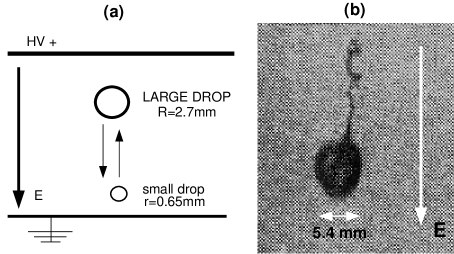
Figure 1: (a) Schematic of Crabb & Latham’s experimental setup in which two drops (R=2.7mm and r=0.65mm) collided in the presence of an applied electric field. (b) Photograph of the coalesced drop that formed after the collision.

Figure 1 (a) shows a schematic of the CL experiment . Their chamber, held at surface pressure, had a positive, high voltage upper plate and a grounded lower plate separated by 50mm. Voltages of up to 30 kV could be applied - corresponding to a maximum uniform E-field of 600 kV/m within the chamber. Large water drops (R=2.7mm) were dropped into the chamber and collided with small drops (r=0.65mm) which were blown upwards, simulating drops moving in updrafts in thunderclouds. A variety of coalesced drop shapes were observed, depending on the nature of the collision. CL described three basic collision modes: head-on, glancing and intermediate. Glancing and intermediate collisions produced a coalesced drop with a long filament extending from the large drop - see Fig 1 (b). Head-on collisions resulted in a flattening of the large drop and did not produce these long filaments. The drops remained in the coalesced state for $\sim$ 1 ms. In CL’s setup, a negative charge was induced on the upper surface of the drop while the lower end had a positive induced charge. In the thundercloud setting these drops would be located above the negative charge center of the cloud. CL recorded the size and shape of the coalesced drops as well as the applied E-fields required to initiate discharges for a large number of coalesced drops. They observed discharges from both ends of the drop but focussed on the positive pulses occurring at the lower surface of the drop. This surface was observed to remain intact. In contrast surface disruption was observed at the upper, negative surface of the drop. CL observed that positive burst pulses occured for values of E between 250 and 500 kV/m, depending on the length of the coalesced drop.

3. Model Description We describe three basic discharge processes that can occur at the surfaces of drops in the presence of strong E-fields. The first process, surface disruption discharge, occurs when the electrostatic repulsive force on a drop in a strong E-field exceeds the surface tension. This results in breakup of the drop surface, and an associated discharge. [Dawson, 1969] observed the surface E-field, $E_{disruption}$, required to initiate this form of discharge as a function of drop size. $E_{disruption}$ is independent of pressure. The remaining processes are referred to as ’pure’ corona processes because the discharge initiates without the occurrence of drop surface disruption. These processes are:

• burst pulse discharges, which are intermittent, and

• continuous streamers, which are capable of propagating continuously.

We discuss each in detail below. All of these processes result in deposition of charge on the drop: either positive or negative charge depending on the sign of $E_{external}$. We focussed only on positive corona: it is simpler to model, has a lower initiation threshold and was studied more extensively by CL than negative corona.

(a) Positive Pure Corona model

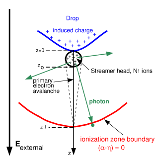
Figure 2: Schematic of positive discharge formation near the surface of a drop. Free electrons are accelerated by the E-field and undergo collisions with air molecules. The ionization of molecules within the ionization zone leads to an exponential growth of electrons (avalanche) and the formation of a spherical streamer head.

Following [Dawson & Winn, 1965, Gallimberti, 1979, Bondiou & Gallimberti, 1994] we model the positive discharge as a series of electron avalanches. Consider the electric field near the surface of a drop which is situated in an external electric field, $E_{external}$. (See Fig 2.) The total electric field is a function of the distance, $r$, from the drop surface. Initially, the total electric field at $r$ is

$$E(r)=E_{g}(r)={E_{external}+E_{drop}(r)}$$ (1)

where $E_{drop}$ is the contribution due to charge induced on the drop. $E_{g}(r)$ is called the geometric field. In the presence of $E$ free electrons are accelerated and undergo collisions with air molecules. At some radial distance from the drop $E$ is such that:

$$\alpha(E/p)=\eta(E/p)$$ (2)

where $\alpha$ [m^-1] and $\eta$ [m^-1] are the ionization and attachment coefficient for electrons in air, respectively and p is the total air pressure. The surface defined by eqn (2) is the ionization zone boundary - inside this boundary $\alpha>\eta$ and there is a net growth of free electrons. At surface pressure the ionization zone boundary is the surface along which $E=2700$ kV/m. Figure 3 shows $\alpha$ and $\eta$ as functions of $E/p$ [Geballe, 1953, Loeb, 1965, Badaloni, 1972, Ibrahim & Singer, 1982].

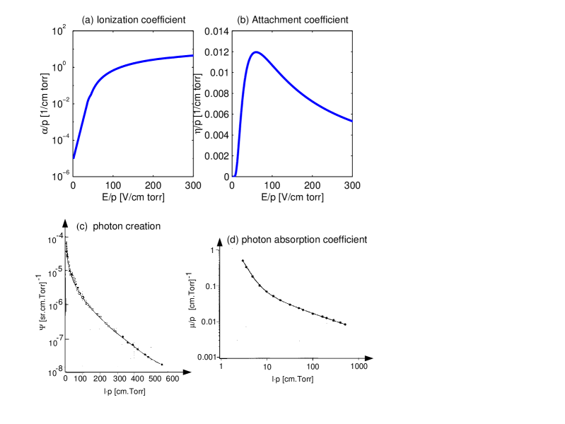
Figure 3: (a) Ratio of ionization coefficient to pressure, $\alpha/p$, for electrons in air [Badaloni, 1972, Loeb, 1965] (b) Ratio of attachment coefficient to pressure, $\eta/p$, for electrons in air [Badaloni, 1972, Geballe, 1953] (c) $\Psi=f_{1}\cdot f_{2}\cdot\theta$ where $f_{1}$ is the number of photons created per ionizing collision, $f_{2}$ [m^-1] is the number of photoions created per photon per meter and $\theta$ is a solid angle = 2$\pi$ in our calculations [Penney & Hummert, 1970] (d) Ratio of photon absorption coefficient to pressure, $\mu/p$, in air [Penney & Hummert, 1970].

Following [Dawson & Winn, 1965, Griffiths & Phelps, 1976, Gallimberti, 1979] we replace the three-dimensional problem by a one-dimensional one in which all avalanches occur along the z-axis. The point $z_{i}$ marks the intersection of the ionization boundary with the $z$-axis. When a free electron, starting at $z_{i}$, is accelerated by $E$ towards the drop, the number of electrons grows exponentially as $z$ decreases. This is referred to as the primary electron avalanche. Due to the exponential nature of the growth, most of the ionizing collisions occur near the surface of the drop. The free electrons are then absorbed by the drop, leaving behind a concentration of positive ions, modeled as a sphere [Dawson & Winn, 1965, Gallimberti, 1979], and referred to as the streamer head. The number of positive ions formed by the primary avalanche traveling from the ionization zone boundary, $z_{i}$, to the drop surface, $z_{o}$, is given by:

$${N_{1}}=exp[\int_{z_{i}}^{o}(\alpha(z))-\eta(z))dz]$$ (3)

The radius of the streamer head is approximately:

$$R_{s}=[6\int\limits_{z_{i}}^{o}(D(z)/{v(z)}dz)]^{1/2}$$ (4)

where $D$ and $v$ are the electron diffusivity and drift velocity, respectively. $D$ and $v$ are functions of the ratio $(E/p)$ and thus depend on $z$ [Healey & Reed,1941, Ibrahim & Singer, 1982]. $R_{s}\approx 30\mu m$ at surface pressure for most of the calculations reported here. The total electric field at $z$ is now given by:

$$E(z)={E_{g}(z)+{eN_{1}\over{4\pi\epsilon_{0}(z-R_{s})^{2}}}}$$ (5)

where the second term, $E_{c}$, is the E-field due to the spherical charge concentration of the streamer head. In addition to ionization, collisions between the free electrons and air molecules also result in the excitation of the molecules, which then emit photons on decay. A certain fraction of these photons in turn have sufficient energy to ionize molecules that they encounter, creating photoelectrons. These photoelectrons then start a series of secondary avalanches which converge on the drop from all directions. The number of photoelectrons created per m at a radial distance, $l$, from the drop surface is given by:

$$P(l)=f_{1}N_{1}\cdot exp[-\mu l]\cdot f_{2}\cdot G$$ (6)

where	$f_{1}$ is the number of photons created per ionizing collision
	$\mu$ [m-1] is the photon absorption coefficient in air
	$f_{2}$ [m-1] is the number of photoions created per photon per meter
	$G$ is a geometric factor to account for the fact that some
	photons are absorbed by the drop.

Both $\mu$ and $f_{1}\cdot f_{2}$ are functions of $l\cdot p$, the product of the distance from the photon source (the collisions) and air pressure [Penney & Hummert, 1970] - see Fig 3. Then the total number of ions created in the secondary avalanches is given by:

$$N_{2}=\int_{z_{i}}^{z_{o}}P(l)\cdot exp[\int_{l}^{z_{o}}(\alpha-\eta)\,dz]\,\,dl$$ (7)

where $z_{o}$ indicates the position of the primary streamer head surface. (i) Initiation Conditions A burst pulse discharge is initiated if the number of photoelectrons created along the ionization zone boundary during the growth of the primary avalanche is equivalent to the number of photoelectrons that started the primary avalanche (commonly taken as 1) [Abdel-Salam et al, 1976]. We consider photoelectron production in a region of depth (1/$\mu$) along the ionization zone boundary and write the above condition as follows:

$$\frac{P(z_{i})}{\mu(z_{i})}=1$$ (8)

This type of discharge is intermittent because the number of positive ions, $N_{1}$, in the primary streamer head is too small to attract the following avalanches to its surface. Instead, the successor avalanches are directed to the drop - allowing the discharge to “spread” over the drop surface. The fulfillment of eqn (8) is strongly influenced by the relationship between the mean free photon path (1/$\mu$) in air and the location of $z_{i}$. For drops with small radii, $z_{i}$ is closer to the drop surface than for those with larger radii. Thus for small drops the number of photons likely to reach the ionization zone boundary is increased. The chances of a photoelectron being produced then increases and it is easier to initiate a burst pulse discharge under these conditions. A more stringent initiation condition exists for continuous streamers. In this case the number of positive ions in the primary streamer head must be large enough to attract the secondary avalanches to the streamer head surface. This is achieved when the radial E-field around the streamer head, $E_{c}=\frac{eN_{1}}{4\pi\epsilon_{0}(z-R_{s})^{2}}\sim E_{g}$ [Abdel-Salam et al, 1976]. In addition:
(a) $N_{2}$, the number of positive ions in the streamer head that results from the secondary avalanches, must equal $N_{1}$, the number of positive ions created by the primary avalanche, and
(b) the radius of the secondary streamer head must equal $R_{s}$, the radius of the primary streamer head.
These conditions ensure that the initial streamer head charge density is reproduced in the second streamer head. Continued reproduction of the streamer head in subsequent steps results in propagation of the positive streamer away from the drop surface. For all the geometric conditions considered in this paper, the initiation of continuous streamers requires a larger external E-field than for burst pulse discharge initiation. The minimum value of $E_{external}$ necessary to initiate a discharge at pressure p is referred to as $E_{initiation}(p)$ and depends on the type of discharge (burst pulse or continuous streamer).

(b) Model Procedure Our results were obtained using the following procedure:

• Define the drop shape and permittivity, $\epsilon$. The idealized shape used is shown in Fig 4. Set the air pressure, p.

• Apply $E_{external}$ to the drop.

• Calculate the E-field distribution around the drop using a finite element method based solving routine [Quickfield].

• Compare the E-field at the drop’s negative surface to the known surface disruption field threshold, $E_{disruption}$ [Dawson, 1969].
  If $E(surface)>E_{disruption}$ then add varying amounts of positive charge, $Q_{drop}$, to the drop.

• Recalculate the E-field distribution [Quickfield].

• Find the ionization zone boundary, $z_{i}$.

• Compute $N_{1}$ and $R_{1}$ from eqns (3) and (4) respectively.

• Compute $P(l)$ at $z_{i}$ from eqn (6).
  For $\frac{P(z_{i})}{\mu(z_{i})}=1,E_{external}=E_{initiation}(p)$ for burst pulse discharges.

• Compute $N_{2}$ and $R_{2}$ from eqns (7) and (4) respectively.
  If $E_{c}\sim E_{g},N_{2}=N_{1}$ and $R_{2}=R_{1}$, then $E_{external}=E_{intiation}(p)$ for continuous streamers.

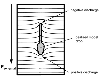
Figure 4: Idealized, model drop used in this study with lines of equipotential shown. The field distribution around the drop is calculated using a finite element method [Quickfield].

4. Results

(a) Surface disruption For $E_{external}\geq$ 200 kV/m the calculated E-field at the surface of the upper, negative end of the drop was $\geq$ 8500 kV/m, the value of $E_{disruption}$ at p=1000mb for a water drop of radius r =0.65mm [Dawson, 1969]. This is consistent with CL’s observations that the upper surface disrupted at these E-field strengths. The resulting negative discharge then deposited positive charge on the drop.

(b) E_initiation vs Q_drop Fig 5 shows the $E_{initiation}$ values for positive burst pulse discharges from the lower positive end of the drop as a function of the charge, $Q_{drop}$, deposited on the drop by the negative discharge from the upper end. The drop length is held fixed at L=20mm.

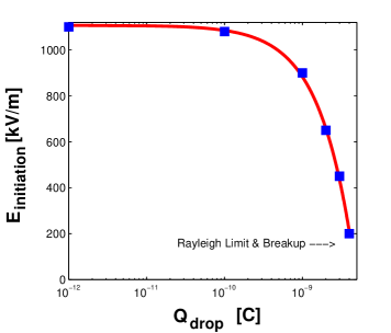
Figure 5: $E_{initiation}$ for positive burst pulse discharges from the lower positive end of the drop as a function of $Q_{drop}$, the charge deposited on the drop by the negative corona from the upper end. The drop length is held fixed at L=20mm.

$E_{initiation}$ decreases rapidly once $Q_{drop}$ exceeds $10^{-10}$ C. The Rayleigh stability criterion [Rayleigh, 1882, Taylor, 1964] gives $Q_{RL}$, the maximum charge that a sphere of liquid can hold before the electrostatic repulsive force overcomes the surface tension. In SI units it is given by:

$$Q_{RL}^{2}=64\,\pi^{2}\,\epsilon_{o}\cdot r^{3}\,\sigma$$ (9)

where r is the sphere radius and $\sigma$ is the surface tension. For our drop dimensions $Q_{RL}\approx 4\times 10^{-9}$ C. Since CL did not observe disruption of the lower surface of the drop, we limited our calculations to $Q_{drop}<Q_{RL}$. For larger allowed values of $Q_{drop}$, close to the Rayleigh limit $Q_{RL}$, the values of $E_{initiation}$ become comparable to CL’s experimental values and to those observed in thunderclouds. In addition to the burst pulse discharges we also calculated the fields required to initiate continuous streamers. For $Q_{drop}$ just below the Rayleigh limit, $E_{initiation}\approx$ 400 kV/m for continuous streamers, approximately 50% greater than that required for burst pulse discharges.

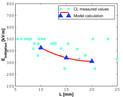
Figure 6: $E_{initiation}$ for burst pulse discharge as a function of the drop length L, for fixed charge density. Triangles: calculated values of $E_{initiation}$ for burst pulse discharges. Circles: Crabb & Latham’s measured values.

(c) E_initiation vs drop length, L We now held the charge density, $\rho$, on the drop fixed at 0.035 C/m³ and varied the drop length, L. The circles in Fig 6 represent CL’s measured values. We found that our modeled values of $E_{initiation}$ for the burst pulse discharges ($\bigtriangleup$) decreased with increasing L, consistent with the trend that CL observed. The agreement between the calculated results and observation is promising and offers validation of our model processes. The scatter in CL’s results is most likely due to either the differences in the shape of the lower end of the coalesced drops or the amount of charge that is deposited by the negative discharge. We found higher $E_{initiation}$ values for a coalesced drop with a spherically shaped lower end, while lower $E_{initiation}$ values were recorded for more pointed lower ends. Our idealized shape with $\rho$=0.035 C/m³, however, provided good agreement with CL’s average values for $E_{initiation}$. The same calculations were carried out for continuous streamers and the results are shown in Fig 7. $E_{initiation}$ decreased with L in much the same way as for burst pulses. The $E_{initiation}$ values for the continuous streamers were, however, $\sim 50\%$ larger than those required for burst pulses.

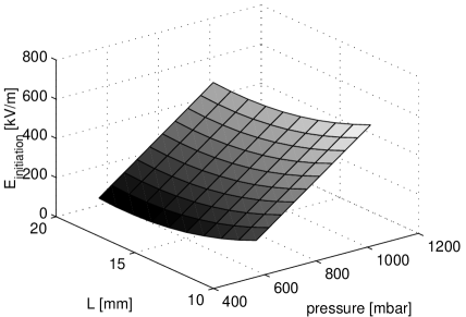
Figure 7: $E_{initiation}$ for continuous discharges as a function of both drop length, L [mm], and pressure, p [mb]

Figure 8 shows the two competing processes that determine the dependence of $E_{initiation}$ on L for continuous streamers. On the one hand, for a given ambient E-field, the surface field at the tip of the filament increases with increasing L, which lowers $E_{initiation}$. In opposition to this, as L increases $E_{g}(z)$ decreases more rapidly with $z$, the distance from the surface. This reduces the size of the ionization zone and thus increases $E_{initiation}$. Fig 7 shows that the former process dominates; i.e. that the increased average field within the ionization zone compensates for the electron’s shortened path - leading to a lowering of $E_{initiation}$ as the filament length is increased. As Fig 7 indicates, $dE_{initiation}/dL$ decreases as L increases and the effect of increased length becomes less significant for L$>$20mm.

Figure 8: E-field as a function of distance, z, from the surface of the drop. E_sl and E_ss are the surface fields for long and short drops, respectively. The ionization zone boundaries for long and short drops are indicated by $z_{il}$ and $z_{is}$, respectively.

(d) The pressure effect All CL’s measurements were made at surface pressure (1000 mb). It is, however, of interest to know what the $E_{initiation}$ values for continuous streamers would be at the lower pressures found in the regions where lightning initiates. We therefore calculated $E_{initiation}$ for continuous streamers for a range of pressures. The variation of $E_{initiation}$ for continuous streamers with both pressure and drop size is shown in Fig 7. The dark region in the lower left corner indicates the region in which initiation is most favorable - large L and low pressure. Over the chosen ranges of pressure and L, pressure has a greater effect on $E_{initiation}$ than L. Fig 7 indicates that $E_{initiation}$ varies linearly with pressure. We consider the dependence of the various parameters used by the model: $\alpha,\eta,D$ and $v$ are functions of $E/p$ while the $\mu$ and $f_{1}\cdot f_{2}$ are functions of $l\cdot p$. The linear dependence of $E_{initiation}$ for continuous streamers suggests that the dependence on $E/p$ dominates and that there is a unique value of the “reduced” E-field, $Y_{initiation}$ = $E_{initiation}/p$ for a particular $E$ and $p$ combination.

(e) Propagation The E-field necessary to sustain stable streamer propagation, $E_{propagation}(p)$, was measured by [Griffiths & Phelps, 1976b] as a function of air pressure, $p$. These stable streamers, once initiated, will continue to propagate provided $E_{initiation}\geq E_{propagation}$. Griffiths and Phelps found that $E_{propagation}\sim 400$ kV/m for dry air at $p=1000$ mb and that $E_{propagation}(p)\propto p^{5}$ (Fig 9). At $p=500$ mb $E_{propagation}\sim 150$ kV/m for dry air.

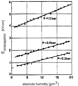
Figure 9: $E_{propagation}$ as a function of absolute humidity and pressure, $p$ [Griffiths & Phelps, 1976b].

At $p=1000mb$ Fig 7 shows that $E_{initiation}>400$ kV/m for all L. These initiated streamers will therefore be able to propagate over the entire length of the region in which $E_{external}$ remains constant. In thunderclouds this scale is typically hundreds of meters. At lower pressures $E_{initiation}>E_{propagation}$ over a large range of L.

5. Discussion In this paper we have shown that continuous, propagating streamers can be initiated from water drops at E-fields found in thunderstorms. Provided that $E_{initiation}(p)\geq E_{propagation}(p)$, these streamers are capable of propagating over considerable distances. This distance is limited by the size of the region in which $E_{external}$ is greater than $E_{propagation}(p)$. When the electron currents in streamers become large enough, Joule heating produces a ’warm’ leader; a channel in which thermodynamic equilibrium is destroyed and hydrodynamic effects become important. This is commonly referred to as the ’stepped-leader’ in the cloud-to-ground lightning context. The currents carried by individual streamers initiated at the drops are several orders of magnitude too low to produce leaders [Bondiou, 1997]. These streamers may, however, still eventually lead to leaders if they can be combined or multiplied. Griffiths & Phelps [1976] considered the role of small scale discharges in thunderclouds, calculating the E-field enhancement due to multiple propagations of positive streamers near an electrode. According to their model, a series of three to seven streamers gave rise to an enhanced E-field of up to $\sim 1500$ kV/m in a region of several meters in linear scale near the electrode. It is possible that several continuous streamers initiated from drops in the thundercloud could provide the required field enhancement. [Griffiths & Phelps, 1976] found that the field was intensified on a time scale of $\sim$ 1 ms, which is comparable to the lifetime of the coalesced drops as measured by CL. Further investigation is required to determine whether a hydrometeor is capable of initiating multiple streamers. An alternate mechanism for leader formation would be the combination of several streamers in close proximity to one another to form a single, more vigorous streamer with sufficient current to transform it to the “warm” leader stage. If we think of drops that initiate continuous streamers as “electrodes” then the number of “electrodes” available increases with increasing E (see Fig 6). Thus the likelihood of several streamers initiating in close proximity increases and the chance of leader formation is increased. This is also in keeping with the observations of large amounts of corona activity in thunderstorms without lightning. Only if the “electrode” density is sufficiently high will streamers be able to merge and form a leader. These possible mechanisms for leader formation require further investigation. The streamers observed by both CL and examined in our model were all positive, occuring at the lower end of drops. This corresponds to drops located above the negative charge center in clouds. Leader formation in this region is observed to lead to intra-cloud lightning flashes. Drops located below the negative charge center have negatively charged lower ends and investigation of this situation will require the modeling of negative streamers which are much more complex in nature than positive streamers [Castellani et al, 1994]. Leader formation in this region (below the negative charge center) will lead to cloud to ground lightning. No attempt has been made in this paper to model these negative processes but future attempts should investigate this phenomena. Finally, while we have concentrated on liquid hydrometeors, future work should incorporate ice particles as possible “electrodes”. This may explain how lightning initiation can occur at higher altitudes near the upper positive charge center in thunderclouds where there is little or no liquid water available.

Acknowledgements We are grateful for support by NASA # NAG8-1150. We thank Anne Bondiou-Clergerie of ONERA for supplying the ionization and attachment coefficient data and providing helpful comments and advice. We are also grateful to Ron Geballe for his suggestions.

References

- [Abdel-Salam et al, 1976] Abdel-Salam, M, A.G. Zitoun and M.M. El-Ragheb, 1976: IEEE Transactions on Power Apparatus and Systems, PAS-95, 1019-1027.
- [Badaloni, 1972] S. Badaloni, 1972: UPee Reoprt, University of Padua, Italy
- [Bondiou, 1997] Bondiou, A., 1997: Private communication
- [Bondiou & Gallimberti, 1994] Bondiou, A. and I. Gallimberti, 1994: J. Phys. D., 27,1252-1266.
- [Castellani et al, 1994] Castellani, A., A. Bondiou, A. Bonamy, P. Lalande and Gallimberti, I: ICOLSE, Mannheim, Germany, May 1994
- [Crabb & Latham, 1974] Crabb, J. and J. Latham, 1974: Q. J. Roy. Met. Soc., 100, 191-202.
- [Dawson, 1969] Dawson, G., 1969: J. Geophys. Res., 74, 6859-6868.
- [Dawson & Winn, 1965] Dawson, G. and W. Winn, 1965: Z. Phys., 183, 159-171.
- [Gallimberti, 1972] Gallimberti, I., 1972: J. Phys. D: Appl. Phys., 5, 2179-2189.
- [Gallimberti, 1979] Gallimberti,I. 1979: J. de Physique , 40, Colloque 7, C7-193, C7-250.
- [Geballe, 1953] Harrison, M.A. and R. Geballe, 1953 Phys. Rev., 91, 1
- [Griffiths & Phelps, 1976] Griffiths, R. and C. Phelps, 1976: J. Geophys. Res., 31, 3671-3676.
- [Griffiths & Phelps, 1976b] Griffiths, R. and C. Phelps, 1976: Q. J. Roy. Met. Soc., 102, 419-426.
- [Healey & Reed,1941] Healey and Reed, 1941: The behavior of Slow Electrons in Gases. Wireless Press, Sidney, Australia.
- [Ibrahim & Singer, 1982] Ibrahim, A.A. and H. Singer, 1982: 7th Int. Conf. on Gas Discharges and their Applications, 128-31.
- [Loeb, 1965] Loeb, L.B., 1965: Electrical Coronas - Their Basic Physical Mechanisms. University of California Press, Berkley, U.S.A.
- [Marshall et al, 1995] Marshall, T., M. McCarthy and W. D. Rust, 1995: J. Geophys. Res., 100, 7097-7103.
- [Penney & Hummert, 1970] Penney, G.W. and G.T. Hummert, 1970: J. Appl. Phys., 41, 572- 577.
- [Quickfield] Quickfield Software, Web address: http://www.tor.ru/quickfield/
- [Rayleigh, 1882] Rayleigh, Lord, 1882: Phil. Mag., 14, 184 - 185.
- [Taylor, 1964] Taylor, G.I., 1964: Proc. Roy. Soc., 280, 383-397.
- [Winn et al, 1974] Winn, W.P., G.W. Schwede and C.B. Moore, 1974 J. Geophys. Res., 79, 1761-1767.