Potential Momentum, Gauge Theory, and Electromagnetism in Introductory Physics

Abstract

If potential energy is the timelike component of a four-vector, then there must be a corresponding spacelike part which would logically be called the potential momentum. The potential four-momentum consisting of the potential momentum and the potential energy taken together, is just the gauge field of the associated force times the charge associated with that force. The canonical momentum is the sum of the ordinary and potential momenta.

Refraction of matter waves by a discontinuity in a gauge field can be used to explore the effects of gauge fields at an elementary level. Using this tool it is possible to show how the Lorentz force law of electromagnetism follows from gauge theory. The resulting arguments are accessible to students at the level of the introductory calculus-based physics course and tie together classical and quantum mechanics, relativity, gauge theory, and electromagnetism. The resulting economy of presentation makes it easier to include modern physics in the one year course normally available for teaching introductory physics.

1 Introduction

Many physicists believe that it is important to introduce more modern physics to students in the introductory college physics course. (See, for instance, the summary of the IUPP project by Coleman et al. [1].) Our experience indicates that retaining the conventional course structure and tacking modern physics on at the end almost guarantees failure in this endeavor, due to the time constraints of the typical one year course. Completely restructuring the course has been tried (see, for instance, Amato [2], Mills [3], Moore [4], Weinberg [5]) and some form of this approach may be the most effective way to accomplish the desired goal.

Raymond and Blyth [6] briefly outlined efforts to develop an introductory college physics course with a radically modern perspective. The first semester of this two semester course begins with optics and waves, proceeds from there to relativistic kinematics, and then introduces the basic ideas of quantum mechanics. It finishes with the development of classical mechanics as the geometrical optics limit of quantum mechanics. The second semester builds on the results of the first semester and covers more mechanics, electromagnetism, a survey of the standard model, and statistical physics.

The structure of this course was inspired by the Nobel Prize address of Louis de Broglie [7]. The logic which led de Broglie to the relation between momentum and wavenumber makes use of a beautiful application of the principle of relativity to obtain the relativistic dispersion relation for waves representing massive particles. Furthermore, de Broglie largely anticipated the development of the Schrödinger equation via an analogy between the propagation of light through a medium of varying refractive index and the propagation of matter waves in a region of spatially variable potential energy.

De Broglie’s approach to matter waves subject to a potential suggests a way of getting these ideas across in elementary form to beginning physics students. We believe that the use of the Schrödinger equation per se is inappropriate at the level of an introductory physics course. However, much of the physics of this equation can be extracted from its dispersion relation in the case where the potential energy is piecewise constant.

The dispersion relation for free matter waves was obtained by de Broglie from little more than the notion of relativistic invariance. Relativity also helps in the development of a modified dispersion relation for matter waves subject to external influences, since the modified as well as the original relation must satisfy relativistic invariance. There turn out to be only a few possible invariant ways to make this modification — gauge theory results from one of these. Pursuit of this choice leads inevitably to the Lorentz force law of electromagnetism. Use of Coulomb’s law and variations on the relativistic invariance arguments of Purcell [9] and Schwartz [10] lead to most of the rest of electromagnetism.

The key arguments in this path involve the derivation and use of variations on Snell’s law to show how wave packets change their velocity when they cross a discontinuity in a gauge field. These arguments invoke the same physics that appears in the application of Hamilton’s principle to the generation of the equations of mechanics, albeit on a much more elementary level. This connection becomes evident when it is realized that Snell’s law contains the same physics as Fermat’s principle, which in turn is an application of the principle of least action.

The above comments explain why we initially study waves and relativity in the introductory course. Mastery of these topics allows even beginning students to obtain at least some insight into the most subtle and profound ideas of physics, insight which can only be acquired via the traditional path after many years of hard work. In addition, it points to an alternative approach to electromagnetism at the introductory level which may actually be easier for beginning students to understand than the traditional approach and is undoubtedly more economical of student time and effort.

2 Potential Momentum

De Broglie treated particles in a potential by developing a formula for the index of refraction $n$ such that wave packets of light would act like such particles. The problem of computing the evolution of matter waves was then reduced to the problem of computing the propagation of light through a medium with variable refractive index. Pursuit of this program leads to the Schrödinger equation.

A great deal can be learned about the propagation of light through a spatially variable medium by examining the case of piece-wise constant index of refraction. In a region in which $n(\mbox{\bf k})$ is independent of position, wave packets of light move according to the group velocity computed from the dispersion relation $\omega=c|\mbox{\bf k}|/n$, where $\omega$ is the angular frequency of the light, $c$ is the speed of light in a vacuum, and k is its wave vector. A wave packet crossing a discontinuity in $n$ is treatable as a problem in refraction.

De Broglie concentrated on the non-relativistic limit in his discussion of the interaction of waves with a potential. However, in some ways the relativistic case is simpler, because any modification to the free particle dispersion relation for relativistic matter waves must also be relativistically invariant. The dispersion relation for free relativistic particles of mass $m$ is

$$\omega^{2}-k^{2}c^{2}=m^{2}c^{4}/\hbar^{2}$$ (1)

where $\hbar$ is Planck’s constant divided by $2\pi$. We write this in the notation of the introductory course as

$$\underline{k}\cdot\underline{k}=-m^{2}c^{2}/\hbar^{2}$$ (2)

where $\underline{k}=(\mbox{\bf k},\omega/c)$ is the wave four-vector with the wave vector k being the spacelike part and $\omega/c$ the timelike part of $\underline{k}$. (We find it advantageous to use Weinberg’s choice of metric [11], $\underline{k}\cdot\underline{k}=\mbox{\bf k}\cdot\mbox{\bf k}-\omega^{2}/c^{2}$, because the four-vector dot product becomes a simple extension of the ordinary dot product with one additional term.)

One can imagine only a few ways to modify equation (2) so as to maintain relativistic invariance:

• One could write

  $$\underline{k}\cdot\underline{k}=-(m-A)^{2}c^{2}/\hbar^{2}$$ (3)

  where $A$ is a relativistic scalar.

• An alternative would be

  $$(\underline{k}-\underline{A})\cdot(\underline{k}-\underline{B})=-m^{2}c^{2}/\hbar^{2}$$ (4)

  where $\underline{A}$ and $\underline{B}$ are four-vectors. Weak, strong, and electromagnetic gauge theories correspond to the case $\underline{A}=\underline{B}$.

• The final apparent possibility is

  $$\underline{k}\cdot\underline{N}\cdot\underline{k}=-m^{2}c^{2}/\hbar^{2}$$ (5)

  where $\underline{N}$ is a tensor which becomes the identity tensor of spacetime in the free particle case.

In the introductory course we state that

$$(\underline{k}-\underline{T})\cdot(\underline{k}-\underline{T})=-m^{2}c^{2}/\hbar^{2}$$ (6)

is the correct choice for all natural forces except gravity. However, we also explore the consequences of a scalar potential field. (The tensor potential is too complex to consider in an introductory course!)

The four-vector gauge field $\underline{T}$ has the form $\underline{T}=(\mbox{\bf T},S/c)$ so that the dispersion relation for matter waves under the influence of a constant gauge field expands to

$$(\omega-S)^{2}-|\mbox{\bf k}-\mbox{\bf T}|^{2}c^{2}=m^{2}c^{4}/\hbar^{2}.$$ (7)

Multiplying this equation by $\hbar^{2}$ leads to the relativistic energy-momentum relationship for particles interacting with a constant gauge field,

$$(E-U)^{2}-|\mbox{\boldmath$\Pi$}-\mbox{\bf Q}|^{2}c^{2}=m^{2}c^{4},$$ (8)

where $\underline{Q}\equiv\hbar\underline{T}=(\mbox{\bf Q},U/c)$. $E=\hbar\omega$ is the total energy and $\mbox{\boldmath$\Pi$}=\hbar\mbox{\bf k}$ is the canonical momentum [8]. However, we refer to it as the total momentum in the introductory course in analogy with the total energy. The quantity $U$ is just the potential energy.

We call the new quantity Q the potential momentum. This terminology arose in a natural way during the first iteration of the introductory course. We had discussed the fact that momentum and kinetic energy together form a four-vector. I then pointed out that potential energy is a quantity much like kinetic energy and asked the class what this implied. A particularly bright freshman replied “…groan, potential momentum!”.

3 Group Velocity and Refraction of Matter Waves

In the introductory class it is necessary at this point to teach the students about partial derivatives, since they typically have not yet covered this concept in their calculus course. However, this is a relatively easy idea to get across. It is also necessary to extend the idea of group velocity (about which they have learned earlier in the section on optics) to more than one dimension. Thus, for instance, in two dimensions we have $\omega=\omega(k_{x},k_{y})$ and the group velocity is

$$\mbox{\bf u}_{g}=\left(\frac{\partial\omega}{\partial k_{x}},\frac{\partial\omega}{\partial k_{y}}\right).$$ (9)

At this stage we find it best to state the above result without proof as a plausible extension of the one-dimensional result.

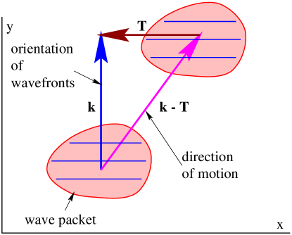
Figure 1: Orientation and motion of a quantum mechanical wave packet in two dimensions. The vector T is perpendicular to the wave vector k in this case.

Given equation (9) it is easy to show that the group velocity of a quantum mechanical wave is just

$$\mbox{\bf u}_{g}=\frac{(\mbox{\bf k}-\mbox{\bf T})c^{2}}{\omega-S}=\frac{(\mbox{\boldmath$\Pi$}-\mbox{\bf Q})c^{2}}{E-U}.$$ (10)

This reduces to the usual expression for the group velocity of relativistic matter waves when Q and $U$ are zero.

An example of the motion of a wave packet is illustrated in figure 1, which shows the student that wave packets don’t necessarily move in the direction of the wave vector when $\mbox{\bf T}\neq 0$.

Eliminating $E-U$ and then $|\mbox{\boldmath$\Pi$}-\mbox{\bf Q}|$ between equations (8) and (10) yields generalizations of the usual formulas for the relativistic momentum and energy,

$$\mbox{\boldmath$\Pi$}=\mbox{\bf Q}+m\mbox{\bf u}_{g}\gamma$$ (11)

$$E=U+mc^{2}\gamma$$ (12)

where $\gamma=(1-u_{g}^{2}/c^{2})^{-1/2}$. We call the ordinary relativistic momentum $\mbox{\bf p}\equiv m\mbox{\bf u}_{g}\gamma$ the kinetic momentum just as $mu_{g}^{2}/2=E-U=K$ is the kinetic energy.

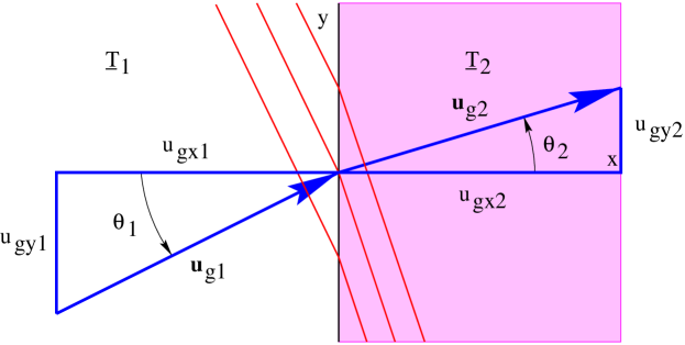
Figure 2: Refraction by a discontinuity in a gauge field $\underline{T}$ at $x=0$.

Figure 2 shows refraction by a discontinuity in a gauge field. The frequency, $\omega$, and the component of the wave vector parallel to the interface, $k_{y}$, are constant across the interface as a result of phase continuity. This implies that $E$ and $\Pi_{y}$ are continuous as well. In the non-relativistic limit $\gamma\approx 1+u_{g}^{2}/(2c^{2})$, and these conditions reduce to the continuity of $U+mu_{g}^{2}/2$ and $Q_{y}+mu_{gy}$ across the interface.

4 Gauge Forces, Non-Relativistic Limit

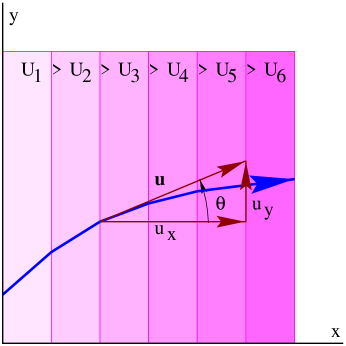
Figure 3: Trajectory of a wave packet through a variable scalar gauge field in which $U=\hbar S$ decreases to the right.

The above expressions are sufficient to infer the accelerations of a particle in the non-relativistic geometrical optics limit, and therefore the forces acting on it. Let us first set $\mbox{\bf Q}=0$ and approximate continuous variability in $U$ along the $x$ axis by a sequence of slabs of constant $U$ as shown in figure 3. In this case $U+mu_{g}^{2}/2$ and $u_{gy}$ are constant. Thus, the $x$ and $y$ components of the force are

$$F_{x} = m\frac{du_{gx}}{dt}=m\frac{du_{gx}}{dx}\frac{dx}{dt}=m\frac{du_{gx}}{dx}u_{gx}$$ (13)

$$= \frac{m}{2}\frac{du_{gx}^{2}}{dx}=\frac{m}{2}\frac{du_{g}^{2}}{dx}=-\frac{dU}{dx}$$

and

$$F_{y}=m\frac{du_{gy}}{dt}=0.$$ (14)

In this case the force is the familiar negative gradient of the potential energy.

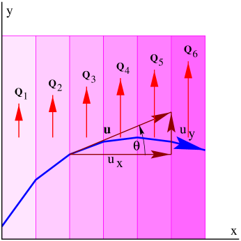
Figure 4: Trajectory of a wave packet through a variable vector gauge field in which $\mbox{\bf Q}=\hbar\mbox{\bf T}$ changes to the right as shown.

Next we set $U=0$ and assume that $\mbox{\bf Q}=(0,Q,0)$, with $Q$ varying as shown in figure 4. Since $Q+mu_{gy}$ is constant in the non-relativistic limit, we see that

$$F_{y}=m\frac{du_{gy}}{dt}=m\frac{du_{gy}}{dx}u_{gx}=-u_{gx}\frac{dQ}{dx}.$$ (15)

However, $mu_{g}^{2}/2=m(u_{gx}^{2}+u_{gy}^{2})/2$ is also constant in this case, from which we infer that

$$F_{x}=m\frac{du_{gx}}{dt}=-m\frac{u_{gy}}{u_{gx}}\frac{du_{gy}}{dt}=-mu_{gy}\frac{du_{gy}}{dx}=u_{gy}\frac{dQ}{dx}.$$ (16)

Putting this together, we find

$$\mbox{\bf F}=\left(u_{gy}\frac{dQ}{dx},-u_{gx}\frac{dQ}{dx},0\right).$$ (17)

This is a special case of the more general result

$$\mbox{\bf F}=\mbox{\bf u}_{g}\times\mbox{\bf P}$$ (18)

where

$$\mbox{\bf P}=\left(\frac{\partial Q_{z}}{\partial y}-\frac{\partial Q_{y}}{\partial z},\frac{\partial Q_{x}}{\partial z}-\frac{\partial Q_{z}}{\partial x},\frac{\partial Q_{y}}{\partial x}-\frac{\partial Q_{x}}{\partial y}\right).$$ (19)

The general case is not proved in the introductory class, but is presented as a plausible generalization of equation (17).

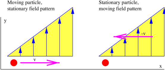
Figure 5: A moving particle and a stationary pattern of potential momentum $\mbox{\bf Q}(x)$ must be equivalent to a stationary particle and a moving pattern of potential momentum according to the principle of relativity.

So far we have assumed that the gauge fields affecting particles are constant in time. An interesting effect occurs when a vector gauge field varies with time. Figure 5 shows how we attack this problem. According to the principle of relativity, the case of a particle moving in the $+x$ direction through a region in which Q is steady with time but increases in magnitude with $x$ is equivalent to the case of a stationary particle in which Q at the particle increases with time. As figure 5 shows, this is because in the latter situation the whole pattern of Q shifts to the left with time, resulting in the particle being exposed to larger and larger values of Q. (We emphasize to our classes that it is important to think of the field pattern as shifting, not the field itself. Fields don’t move, they just have space and time variations which look different in different reference frames.) The time rate of change of Q at the position of the particle in the right panel of figure 5 is

$$\frac{\partial\mbox{\bf Q}}{\partial t}=\frac{\partial Q}{\partial x}\frac{dx}{dt}=v\frac{\partial\mbox{\bf Q}}{\partial x}.$$ (20)

Equation (17) applies to the left panel of figure 5 with $u_{gx}=v$, $u_{gy}=0$ and $\mbox{\bf Q}=(0,Q,0)$. The resulting force on the object is $\mbox{\bf F}=-v(\partial\mbox{\bf Q}/\partial x)$. However, by the principle of relativity, the force on the object in the right panel should be the same. (We are assuming low velocity transformations, so the issue of F possibly changing as a result of the transformation doesn’t arise here.) We therefore infer that the force on a stationary particle with time-varying Q is

$$\mbox{\bf F}=-\frac{\partial\mbox{\bf Q}}{\partial t}.$$ (21)

Putting all these effects together, the complete gauge force is thus written

$$\mbox{\bf F}=-\frac{\partial\mbox{\bf Q}}{\partial t}-\left(\frac{\partial U}{\partial x},\frac{\partial U}{\partial y},\frac{\partial U}{\partial z}\right)+\mbox{\bf u}_{g}\times\mbox{\bf P},$$ (22)

in the non-relativistic case, which is recognizable as being only a step away from the Lorentz force law for electromagnetism. If the charge on the particle is $q$, then the scalar potential is $\phi=U/q$, the vector potential is $\mbox{\bf A}=\mbox{\bf Q}/q$, the electric field E is the first two terms on the right side of the above equation divided by $q$, and the magnetic field is $\mbox{\bf B}=\mbox{\bf P}/q$. Thus, using only elementary arguments, the Lorentz force is shown to be a consequence of the gauge theory assumption, which in turn arises from the assumption of a potential momentum.

5 Electromagnetism

Purcell [9] and Schwartz [10] infer the character of electromagnetic fields from moving charges by performing a Lorentz transformation on configurations of stationary charges. This trick becomes considerably easier when attention is focused on the four-potential $\underline{a}=(\mbox{\bf A},\phi/c)$ rather than on the electric and magnetic fields, because the transformation properties of the four-potential are much simpler.

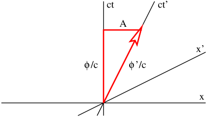
Figure 6: Finding the space and time components of the four-potential which points in the time-like direction in the primed reference frame. The $ct^{\prime}$ axis is the world line of the charge which generates the four-potential. The primed frame moves to the right at speed $v$.

Figure 6 illustrates the idea. The four-potential in this figure points along the $ct^{\prime}$ axis and has invariant length $\phi^{\prime}/c$. Since the primed reference frame moves to the right at speed $v$, the components of the four-potential in the unprimed frame are $\underline{a}=[(\beta\gamma\phi^{\prime}/c)\mbox{\bf i},\gamma\phi^{\prime}/c]$ where $\beta=v/c$, $\gamma=(1-\beta^{2})^{-1/2}$, and i is the unit vector in the $x$ direction.

Figure 7: Vector potential from a moving line of charge. The distribution of vector potential around the line is cylindrically symmetric.

Let us consider a line of charge along the $x$ axis moving with the primed reference frame. In this reference frame we define the linear charge density to be $\lambda^{\prime}$ and find by the usual Gauss’s law techniques plus a simple integration that the scalar potential in the primed frame is

$$\phi^{\prime}=-\frac{\lambda^{\prime}}{2\pi\epsilon_{0}}\ln r$$ (23)

where $r$ is the distance from the $x$ axis. We immediately infer from figure 6 that the vector potential in the unprimed frame is

$$\mbox{\bf A}=-\frac{\beta\gamma\lambda^{\prime}\mbox{\bf i}}{2\pi\epsilon_{0}c}\ln r=-\frac{v\lambda\mbox{\bf i}}{2\pi\epsilon_{0}c^{2}}\ln r,$$ (24)

where $\lambda=\gamma\lambda^{\prime}$ is the Lorentz-contracted charge density in this frame. The vector potential is illustrated in figure 7 and is easily shown to yield the classical result for the magnetic field due to a current $i=v\lambda$:

$$|\mbox{\bf B}|=\frac{v\lambda}{2\pi\epsilon_{0}c^{2}r}=\frac{\mu_{0}i}{2\pi r}.$$ (25)

We have used $\epsilon_{0}\mu_{0}=c^{-2}$ where $\mu_{0}$ and $\epsilon_{0}$ are the permeability and permittivity of free space.

6 Discussion

Some may question the heavy dependence on arguments based on relativity in the present approach. However, our experience has been that relativity is avidly absorbed and understood even by average beginning students when presented in terms of spacetime triangles and a “spacetime Pythagorean theorem” rather than in terms of the rather more abstract Lorentz transformations. Four-vectors don’t seem to present any particular problems and arguments based on relativistic invariance seem to resonate with the students. In this respect our experiences are similar to Moore’s [12].

Others may point out that our treatment of gauge theory leaves out the connection between gauge invariance and the form of the Lagrangian. We confess to not having figured out how to present this result in a way which makes sense to the average college freshman. However, we do point out (in a problem set) that the form of the four-potential leading to particular electric and magnetic fields is not unique. Furthermore, our approach makes non-classical phenomena such as the Aharonov-Bohm effect relatively easy for beginning students to understand.

There are at least three major advantages to the presentation proposed here:

1. Certain aspects of gauge theory are touched upon in a way that makes sense to a beginning student. This is desirable in that the nearly universal role of gauge theory in representing the forces of nature is otherwise hard to describe in a non-trivial way at an introductory level.

2. Our route is arguably a more compact and insightful way to approach electromagnetism than the normal presentation. This is an important consideration given the limited time typically available to the introductory course.

3. The mathematics used here is arguably simpler than is seen in typical presentations of the mechanics of conservative forces and electromagnetism. In particular, though partial derivatives are introduced, the use of the line integral, a particularly puzzling concept for beginning students, is completely avoided.

Our approach thus fosters the goal of presenting the most profound ideas of physics in a manner that is as accessible as possible to beginning students.

Acknowledgments: Particular thanks go to Robert Mills of Ohio State University for pointing out a serious error in an earlier version of this paper.

References

- [1] L. A. Coleman, D. F. Holcomb, and J. S. Rigden, “The Introductory University Physics Project 1987-1995: What has it accomplished?”, Am. J. Phys. 66, 124-137 (1998).
- [2] J. Amato, “The Introductory Calculus-Based Physics Textbook”, Physics Today, 46-50, (December 1996).
- [3] R. Mills, Space Time and Quanta (Freeman, New York, 1994).
- [4] T. Moore, Six Ideas that Shaped Physics (McGraw-Hill, New York, publication pending).
- [5] S. Weinberg, The Discovery of Subatomic Particles (Freeman, New York, 1983).
- [6] D. J. Raymond and A. M. Blyth, (Letter to the Editor), Physics Today, 92-94, (April 1997).
- [7] L. V. de Broglie, The Undulatory Aspects of the Electron (Nobel Prize Address, Stockholm, 1929, reprinted in H. A. Boorse and L. Motz, The World of the Atom, (Basic Books, New York, 1966)).
- [8] H. Goldstein, Classical Mechanics (Addison-Wesley, Reading, Mass., 1950).
- [9] E. M. Purcell, Electricity and Magnetism (McGraw-Hill, New York, 1963).
- [10] M. Schwartz, Principles of Electrodynamics (McGraw-Hill, New York, 1972).
- [11] S. Weinberg, The Quantum Theory of Fields, Vol. I, Foundations (Cambridge U. P., Cambridge, 1995).
- [12] T. A. Moore, A Traveler’s Guide to Spacetime (McGraw-Hill, New York, 1995).