On the Dynamical Stability of the Hovering Magnetic Top

Abstract

In this paper we analyze the dynamic stability of the hovering magnetic top from first principles without using any preliminary assumptions. We write down the equations of motion for all six degrees of freedom and solve them analytically around the equilibrium solution. Using this solution we then find conditions which the height of the hovering top above the base, its total mass, and its spinning speed have to satisfy for stable hovering.

The calculation presented in this paper can be used as a guide to the analysis and synthesis of magnetic traps for neutral particles.

1 Introduction

1.1 The hovering magnetic top.

The hovering magnetic top is an ingenious device that hovers in mid-air while spinning. It is marketed as a kit in the U.S.A. and Europe under the trade name Levitron${}^{\mbox{TM}}$ [1, 2] and in Japan under the trade name U-CAS[3]. The whole kit consists of three main parts: A magnetized top which weighs about 18gr, a thin (lifting) plastic plate and a magnetized square base plate (base). To operate the top one should set it spinning on the plastic plate that covers the base. The plastic plate is then raised slowly with the top until a point is reached in which the top leaves the plate and spins in mid-air above the base for about 2 minutes. The hovering height of the top is approximately 3cm above the surface of the base whose dimensions are about 10cm$\times$10cm$\times$2cm. The kit comes with extra brass and plastic fine tuning weights, as the apparatus is very sensitive to the weight of the top. It also comes with two wedges to balance the base horizontally.

1.2 Qualitative Description.

The physical principle underlying the operation of the hovering magnetic top relies on the so-called ‘adiabatic approximation’ [4, 5, 6, 7]: As the top is launched, its magnetization points antiparallel to the magnetization of the base in order to supply the repulsive magnetic force which will act against the gravitational pull. As the top hovers, it experiences lateral oscillations which are slow ( $\Omega_{\mbox{lateral}}\simeq 1$Hz) compared to its precession ($\Omega_{\mbox{precession}}\sim 5$Hz). The latter, itself, is small compared to the top’s spin ($\Omega_{\mbox{spin}}\sim 25$Hz). Since $\Omega_{\mbox{spin}}\gg\Omega_{\mbox{precession}}$ the top is considered ‘fast’ and acts like a classical spin. Furthermore, as $\Omega_{\mbox{precession}}\gg\Omega_{\mbox{lateral}}$ this spin may be considered as experiencing a slowly rotating magnetic field. Under these circumstances the spin precesses around the local direction of the field (adiabatic approximation) and, on the average, its magnetization ${\bf\mu}$ points antiparallel to the local magnetic field lines. In view of this discussion, the magnetic interaction energy which is normally given by $-{\bf\mu}\cdot{\bf H}$ is now given approximately by $\mu\left|{\bf H}\right|$. Thus, the overall effective energy seen by the top is

$$E_{\mbox{eff}}\simeq mgz+\mu\left|{\bf H}\right|.$$ (1)

By virtue of the adiabatic approximation, two of the three rotational degrees of freedom are coupled to the transverse translational degrees of freedom, and as a result the rotation of the axis of the top is already incorporated in Eq.(1). Thus, under the adiabatic approximation, the top may be considered as a point-like particle whose only degrees of freedom are translational. The important point of this discussion is the following: The energy expression written above possesses a minimum for certain values of $\mu/m$. Thus, when the mass is properly tuned, the apparatus acts as a trap, and stable hovering becomes possible.

As mentioned above, the adiabatic approximation holds whenever $\Omega_{\mbox{spin}}\gg\Omega_{\mbox{precession}}$ and $\Omega_{\mbox{precession}}\gg\Omega_{\mbox{lateral}}$. As $\Omega_{\mbox{precession}}$ is inversely proportional to $\Omega_{\mbox{spin}}$, these two inequalities can be satisfied simultaneously provided that the top is spun fast enough, to get $\Omega_{\mbox{spin}}\gg\Omega_{\mbox{precession}}$, but not too fast, for then $\Omega_{\mbox{precession}}>\Omega_{\mbox{lateral}}$!. The reason for the lower bound on the spin is obvious: If the top is spun too slowly, then $\Omega_{\mbox{spin}}\lesssim\Omega_{\mbox{precession}}$ and the top becomes unstable against rotations. The top will then flip over and will be pulled quickly to the base. This is the instability that is well known from classical top physics[11, 12]. The reason for an upper bound on the spin is quite different: If the top is spun too fast, the axis of the top becomes too rigid and cannot respond fast enough to the changes of the direction of the magnetic field. It is then considered as fixed in space and, according to Earnshaw’s theorem[10] , becomes unstable against translations.

1.3 The purpose and structure of this paper.

The major problem with the adiabatic approximation is that it cannot predict exactly the allowed range of $\Omega_{\mbox{spin}}$ for which stable hovering occurs. It simply gives us estimates for this range, and for design purposes this may not be enough. The purpose of this paper is to give a quantitative description of the physics of the hovering magnetic top while it is in mid-air without using any preliminary assumptions (such as the adiabatic approximation). To do this, we first expand the magnetic field around the equilibrium point to second order in the spatial coordinates. Using the gradients of this field we then find the force and torque on the top and write down the equations of motion for all 6 degrees of freedom in vectorial form[8]. Next, we solve these equations for the stationary solution and for a small perturbation around this stationary solution and arrive at a secular equation for the frequencies of the various possible modes. The possible eigenmodes are either oscillatory (corresponding to stable solution) or exponential (unstable solution). The secular equation comes out linear in $\Omega_{\mbox{spin}}$, and it is not difficult to write analytic expressions for the upper and lower bounds of $\Omega_{\mbox{spin}}$.

The structure of this paper is as follows: In Sec.2 we first describe our model and define our notations. Next, we derive the equations of motion for the translational and rotational degrees of freedom, and finally we solve these equations around the equilibrium position. In Sec.3 we apply our results to the case of a disk-like top of radius $a=0.25R$ hovering above a circular current loop of radius $R$. We fix the equilibrium hovering height and plot the various frequencies of the stable modes as a function of $\Omega_{\mbox{spin}}$. We identify the origin of the various modes and comment on the way these modes are coupled to produce the minimum and maximum speeds at which the system becomes unstable. In particular the connection of these results with the adiabatic approximation will be discussed. Then we change the equilibrium height and note how the allowed range of $\Omega_{\mbox{spin}}$ is affected. We shall show that above a particular height, where according to the adiabatic approximation hovering is not possible, hovering is still possible in a certain range, and that, furthermore, the lower bound on $\Omega_{\mbox{spin}}\,$originates from a new mode coupling, not predicted by the adiabatic approximation. In the last section we summarize our results and discuss the possible uses of the derivation presented in this paper to the study of magnetic traps for neutral particle.

2 Derivation and Solution of the Equations of Motion.

2.1 Description of the model and notation.

In this paper we analyze the dynamics of the top while in mid-air as is shown in Fig.1. We consider a symmetric top with mass $m$ and a magnetic moment $\mu$, rotating about its principal axis with angular speed $\Omega_{s}$. The magnetic moment of the top is assumed to be concentrated at the center of gravity of the top and to point along the symmetry axis of the top. The latter is denoted by the unit vector ${\bf\hat{n}}$. The moment of inertia of the top about ${\bf\hat{n}}$ is $I_{3}\,$whereas the secondary moment of inertia is $I_{1}$.

The spatial position of the top is given with respect to its equilibrium position (point Q in the figure). Thus, $z$ is the vertical displacement of the top and $\rho$ is its radial displacement. We denote by ${\bf\hat{z}}$ and ${\bf\hat{\rho}}$ the unit vectors in the vertical and radial direction, respectively.

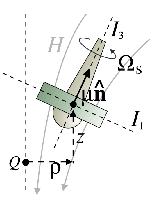
Figure 1: The hovering magnetic top near its equilibrium position (point Q) and notations.

Though this is not mandatory for our calculations, we assume for simplicity, that the magnetic field possesses cylindrical symmetry around the vertical axis. In addition, the direction of gravity is assumed to coincide with the symmetry axis of the magnetic field and to point downward. We denote by $g$ the free fall acceleration.

2.2 The equations of motion.

As the symmetry axis of the magnetic field coincides with the direction of gravity, equilibrium is possible only along this axis. We therefore express the magnetic field, to second order in $\rho$ and $z$, at the vicinity of the equilibrium position in terms of its derivatives along the ${\bf\hat{z}}$ direction at the equilibrium position. This is possible due to cylindrical symmetry and to the fact that the Cartesian components of the field are harmonics. The result is

$${\bf H}(\rho,z){\bf=-}\frac{1}{2}\rho\left(H^{\prime}+H^{\prime\prime}z\right){\bf\hat{\rho}}+\left[H+H^{\prime}z+\frac{1}{2}H^{\prime\prime}\left(z^{2}-\frac{1}{2}\rho^{2}\right)\right]{\bf\hat{z}}\mbox{.}$$ (2)

Here $H$, $H^{\prime}$ and $H^{\prime\prime}$ are the vertical magnetic field, its first and second derivatives along the $\hat{z}$ direction, respectively, at the equilibrium position, i.e. at point Q.

The potential energy of the top is the sum of the magnetic interaction energy of a dipole with a field plus a gravitational term, i.e.

$$E=-\mu{\bf\hat{n}}\cdot{\bf H}\left(\rho,z\right)+mgz\mbox{.}$$

Consequently the force on the top is

$${\bf F}=-{\bf\nabla}E=\mu{\bf\nabla}\left({\bf\hat{n}}\cdot{\bf H}\right)-mg{\bf\hat{z}}\mbox{,}$$ (3)

whereas the torque is

$${\bf T}=\mu{\bf\hat{n}}\times{\bf H}\mbox{.}$$ (4)

The equation for ${\bf r=}\rho{\bf\hat{\rho}+}z{\bf\hat{z}}$, the radius vector of the center of mass of the top with respect to point Q, is given by

$$m\frac{d^{2}{\bf r}}{dt^{2}}{\bf=}\mu{\bf\nabla(\hat{n}\cdot H)-}mg{\bf\hat{z}}\mbox{.}$$ (5)

To write a vectorial equation of motion (see for example [9]) for the angular momentum, ${\bf L}$ , we note that it has two components in perpendicular directions. The first component is due to the rotation of the top around the ${\bf\hat{n}}$ direction and is given simply by ${\bf L}_{n}=I_{3}\Omega_{s}{\bf\hat{n}}$. The second component of the angular momentum is contributed by the change in the direction of the principal axis from ${\bf\hat{n}}$ to ${\bf\hat{n}+}d{\bf\hat{n}}$. Since, by definition, ${\bf\hat{n}}$ is a unit vector, it must point perpendicular to $d{\bf\hat{n}}$. Thus, $\Omega_{\perp}=\left|d{\bf\hat{n}/}dt\right|$ is the angular velocity associated with the change of ${\bf\hat{n}}$. Since the direction of $\Omega_{\perp}$ must be perpendicular to both $d{\bf\hat{n}}$ and ${\bf\hat{n}}$ we form the cross product ${\bf\Omega}_{\bot}={\bf\hat{n}\times}\left(d{\bf\hat{n}/}dt\right)$ which incorporates both the correct value and the right direction. Multiplying ${\bf\Omega}_{\bot}$ by $I_{1}$ yields the second component of the orbital angular momentum, ${\bf L}_{\perp}=I_{1}{\bf\hat{n}\times}\left(d{\bf\hat{n}/}dt\right)$. Thus, ${\bf L=L}_{n}+{\bf L}_{\perp}=$ $I_{3}\Omega_{s}{\bf\hat{n}+}I_{1}{\bf\hat{n}\times(}d{\bf\hat{n}}/dt)$. Using this expression together with Eq.(4) for the torque we find that the equation of motion for the angular momentum is

$$\frac{d{\bf L}}{dt}=\frac{d}{dt}\left[I_{3}\Omega_{s}{\bf\hat{n}+}I_{1}{\bf\hat{n}\times}\frac{d{\bf\hat{n}}}{dt}\right]=\mu{\bf\hat{n}}\times{\bf H}\mbox{.}$$ (6)

Eqs.5,6 together form a coupled system of equations for all 6 degrees of freedom of the top. In these equations ${\bf r}$, ${\bf\hat{n}}$ and $\Omega_{s}$ are the dynamical variables (a total of 6 degrees of freedom), ${\bf H}$ is the magnetic field which itself is a function of ${\bf r}$, whereas $m$, $\mu$, $I_{1}$ and $I_{3}$ are external parameters.

2.3 Solution for the equations of motion

The stationary solution of the problem is obvious: When the top is on the symmetry axis with its principal axis parallel to the ${\bf\hat{z}}$ axis, two forces act on the top. The first force is the downward gravitational force $mg$ and the second one is the upward magnetic force supplied by the external magnetic field, i.e., $\mu H^{\prime}$. Since these forces are colinear, no torque is exerted. We therefore look for a solution of the form

$$\begin{array}[]{c}\rho(t)=z(t)=0\\ {\bf\hat{n}}(t)={\bf\hat{z}}\\ \Omega_{s}(t)=\Omega_{s}=\mbox{Const.}\end{array}$$ (7)

Inserting this solution into Eqs.5,6 yields identities for 5 degrees of freedom. The equation for $z$, on the other hand, gives the expected equilibrium condition

$$\mu H^{\prime}=mg\mbox{.}$$ (8)

To investigate the stability of the stationary solution, we now add first order perturbations to the equations of motion. Thus, we make the following substitutions

$$\begin{array}[]{c}z(t)\rightarrow 0+\delta z(t)\\ {\bf\vec{\rho}}(t)\rightarrow 0+\delta{\bf\vec{\rho}}(t)\\ \Omega_{s}(t)\rightarrow\Omega_{s}(t)+\delta\Omega(t)\\ {\bf\hat{n}}(t)\rightarrow{\bf\hat{z}}+\delta{\bf\hat{n}}(t)\end{array}$$ (9)

where, since ${\bf\hat{n}}$ is a unit vector, $\delta{\bf\hat{n}}$ must be perpendicular to ${\bf\hat{z}}$. Substituting Eq.9 into Eqs.5,6 and expanding to first order in the perturbations gives

$$m\frac{d^{2}\delta{\bf\vec{\rho}}}{dt^{2}}=-\frac{1}{2}\mu H^{\prime}\delta{\bf\hat{n}}-\frac{1}{2}\mu H^{\prime\prime}\delta{\bf\vec{\rho}}$$ (10)

$$m\frac{d^{2}\delta z}{dt^{2}}=\mu H^{\prime\prime}\delta z$$ (11)

$$\frac{d\delta\Omega}{dt}=0$$ (12)

$$I_{3}\Omega_{s}\frac{d\delta{\bf\hat{n}}}{dt}+I_{1}{\bf\hat{z}}\times\frac{d^{2}\delta{\bf\hat{n}}}{dt^{2}}=-\mu H{\bf\hat{z}}\times\delta{\bf\hat{n}}-\frac{1}{2}\mu H^{\prime}{\bf\hat{z}}\times\delta{\bf\vec{\rho}}\mbox{.}$$ (13)

We note that (at least to lowest order) the motions in the $\hat{z}$ direction and the rotation around the ${\bf\hat{n}}$ axis are decoupled from the other degrees of freedom. Furthermore, according to Eq.11 the motion in the $\hat{z}$-direction is stable provided that $H^{\prime\prime}<0$. We now focus our attention on the remaining four degrees of freedom: Note that the right-hand side of Eq.10 contains two terms: The first is the adiabatic term which tends to stabilize the top against lateral translations by tilting the axis of the top. The second term, which we call Earnshaw’s term, tends to destabilize the top and to take it away from the equilibrium position. Solving Eq.10 for $\delta{\bf\hat{n}}$ and substituting it into Eq.13 results in a fourth order equation for the radius $\delta{\bf\vec{\rho}}$:

$$\begin{array}[]{c}2mI_{1}\hat{z}\times\delta{\bf\vec{\rho}}^{(4)}+2mI_{3}\Omega_{s}\delta{\bf\vec{\rho}}^{(3)}+\\ +\mu\left[I_{1}H^{\prime\prime}+2mH\right]\hat{z}\times\delta{\bf\vec{\rho}}^{(2)}+\mu I_{3}\Omega_{s}H^{\prime\prime}\delta{\bf\vec{\rho}}^{(1)}\\ -\mu^{2}\left[\frac{1}{2}\left(H^{\prime}\right)^{2}-HH^{\prime\prime}\right]\hat{z}\times\delta{\bf\vec{\rho}}=0\end{array}\mbox{.}$$ (14)

The possible solutions of this equation are linear combinations of a steady rotation of $\delta{\bf\vec{\rho}}$ around $\hat{z}$ at angular velocity $\omega$ (this is possible because of the cylindrical symmetry of the field; otherwise, one should write two equations for the two components of $\delta{\bf\vec{\rho}}$). We thus set

$$\frac{d\delta{\bf\vec{\rho}}}{dt}=\omega\hat{z}\times\delta{\bf\vec{\rho}}\mbox{.}$$ (15)

Substitution of Eq.15 into Eq.14 results in the following secular equation for the eigenfrequencies:

$$\begin{array}[]{c}2mI_{1}\omega^{4}-2mI_{3}\Omega_{s}\omega^{3}\\ -\mu\left[I_{1}H^{\prime\prime}+2mH\right]\omega^{2}+\mu I_{3}\Omega_{s}H^{\prime\prime}\omega\\ -\mu^{2}\left[\frac{1}{2}\left(H^{\prime}\right)^{2}-HH^{\prime\prime}\right]=0\mbox{.}\end{array}$$ (16)

This fourth-order equation for $\omega$ has four real roots (or eigenfrequencies) whenever the system is stable. Since we are looking for the range of $\Omega_{s}$ for which the system is stable, we take another point of view and express $\Omega_{s}$ in terms of $\omega$. The resulting equation after using $mg=\mu H^{\prime}$ is

$$\Omega_{s}=\frac{2I_{1}H^{\prime}\omega^{4}-g\left[I_{1}H^{\prime\prime}+2mH\right]\omega^{2}-mg^{2}\left[\frac{1}{2}H^{\prime}-\frac{HH^{\prime\prime}}{H^{\prime}}\right]}{2I_{3}H^{\prime}\omega^{3}-gI_{3}H^{\prime\prime}\omega}\mbox{.}$$ (17)

3 Application to a disk-like top above a circular current loop.

As an example we now apply Eq.17 to the case of a disk-like top of radius $a$. Consequently, $I_{3}=ma^{2}/2$ and $I_{1}=ma^{2}/4$. The source of the magnetic field is taken as a horizontal current loop (or alternatively, a vertically uniformly magnetized thin disk) of radius $R$. The vertical magnetic field and its derivatives along the axis at a height $h$ above the loop are therefore given by

$$\begin{array}[]{c}H=-H_{0}\left[1+\left(h/R\right)^{2}\right]^{-3/2}\\ H^{\prime}=\frac{3H_{0}}{R}\left(h/R\right)\left[1+\left(h/R\right)^{2}\right]^{-5/2}\\ H^{\prime\prime}=\frac{3H_{0}}{R^{2}}\left[1-4\left(h/R\right)^{2}\right]\left[1+\left(h/R\right)^{2}\right]^{-7/2}\mbox{.}\end{array}$$ (18)

Note that the magnetic field was chosen to point downward. Thus, in order to get an upward repulsive magnetic force, the magnetic moment should point upward. The sign convention is chosen such that $h$ and $\mu$ are positive, $H$ is negative and, consequently, $H^{\prime}$ is positive. For stability in the $z$ direction we require $H^{\prime\prime}<0$. This occurs, according to Eq.18, as long as $h>h_{\min}=0.5R,$ and sets a lower bound for the height at which stable hovering is possible. Taking $h=0.55R$ and $a=0.25R$ (these are approximately the parameters for the Levitron) inside Eq.17 and plotting $\Omega_{s}$ versus $\omega$ yields the solid line shown in Fig.2. Note that both $\Omega_{s}$ and $\omega$ are normalized to $\omega_{0}=\sqrt{g/R}$.

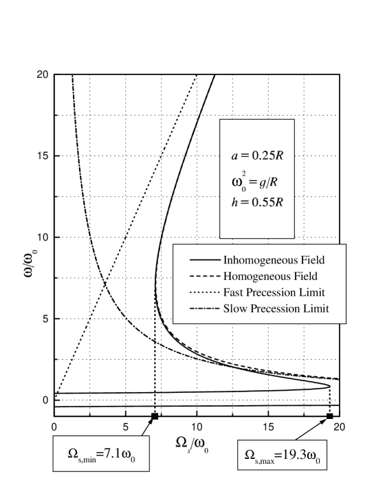
Figure 2: Mode frequencies vs. spin for a disk-like top of radius $a$ hovering at a height $h$ above a circular current loop of radius $R$. Solid line: inhomogeneous field, dashed line: homogeneous field, dotted line: fast precession limit, dashed-dotted line: slow precession limit.

From this figure we learn that (for $h=0.55R$ and $a=0.25R$) whenever

$$7.1\sqrt{g/R}<\Omega_{s}<19.3\sqrt{g/R}$$

there are four real solutions $\omega$ which correspond to four stable modes. The frequency of the fastest mode goes asymptotically to the dotted line $\Omega_{s}=\left(I_{1}/I_{3}\right)\omega$ as $\Omega_{s}\gg\omega_{0}$. This is nothing but the ‘fast precession’ rotational mode encountered in classical top physics[11]. The frequency of the next fastest mode goes roughly like $\omega\simeq\mu H/I_{3}\Omega_{s}$ (compare it to the dash-dash-dotted line). This is the well known ‘slow precession’ rotational mode of a classical top[11]. The coupling between these two modes produces the minimum speed for stability $\Omega_{s,\min}=7.1\sqrt{g/R}$. For comparison purposes we have also included in our plot (dashed line) the resultant mode frequencies when we set $H^{\prime}$ and $H^{\prime\prime}$ $=0$ inside Eq.(16). This is equivalent to solving the problem of a magnetized top, in a homogeneous magnetic field. In fact, these mode frequencies may be obtained as the roots of $\Omega_{s}=\left(I_{1}/I_{3}\right)\omega+\mu H/I_{3}\omega$. The minimum value of this expression occurs for $\omega^{2}=\mu H/I_{1}$ and is given by $\Omega_{s,\min}=\sqrt{4\mu HI_{1}/I_{3}^{2}}$ , which is the minimum speed of a classical top in a homogeneous field. By comparing the mode frequencies for the homogeneous field to the mode frequencies for the inhomogeneous field we see that (as far as the minimum speed is concerned) the minimum speed in both graphs is almost the same. The two slowest modes in the solid-line plot are the two vibrational modes of the top. It is clearly seen that one of them is strongly coupled to the slow precession mode. This coupling is responsible for producing the maximum speed for stability $\Omega_{s,\mbox{max}}=19.3\sqrt{g/R}$, as was already predicted by the adiabatic approximation. But unlike in the adiabatic approximation, we now have a way to find analytically both the minimum and maximum speed in a single stroke.

Our next step is to study how the allowed range of $\Omega_{s}$ depends on the equilibrium height $h$. In Fig.3 we have plotted the mode frequencies versus $\Omega_{s}$ for $h=0.55R,$ $0.6R,$ $0.6325R$ , $0.64R$ and $0.65R$.

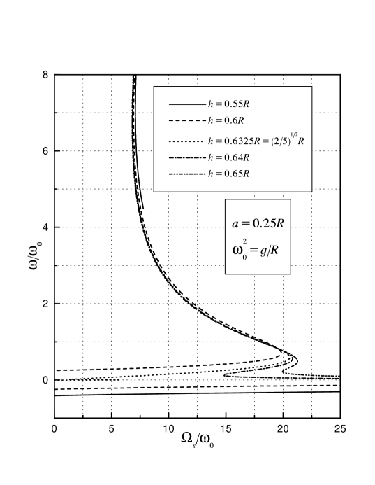
Figure 3: Mode frequencies vs. spin for a disk-like top of radius $a$ hovering at a height $h=0.55R,$ $0.6R$, $0.6325R,$ $0.64R$ and $0.65R$ above a circular current loop of radius $R$.

In Fig.4 we have plotted the minimum and maximum speeds for each equilibrium height starting at $h=0.5R.$ Recall that stability along the ${\bf\hat{z}}$ direction requires that $h>0.5R$. Thus, the two curves plotted in Fig.4 together with the $h=0.5R$ line define a closed region in the $\Omega_{s}$-$h$ plane. Each point inside this region corresponds to a stable hovering solution whereas each point outside this region belongs to an unstable solution. From this figure we may deduce that the range of heights for which stable hovering is possible is given by

$$0.5R\leq h\leq 0.658R$$

The figure also shows that as $h$ increases above its minimum value $h_{\mbox{min}}=0.5R$, the minimum allowed speed $\Omega_{s,\mbox{min1}}$ decreases slightly, whereas the maximum allowed speed $\Omega_{s,\mbox{max}}$ increases. As $h$ increases further, the coupling between the two vibrational modes becomes stronger, and when $h$ exceeds a first critical value $h_{c,1}=\sqrt{2/5}R$, this coupling gives rise to the appearance of a new minimum $\Omega_{s,\mbox{min2}}$ of $\Omega_{s}\left(\omega\right)$, which increases steeply with increasing $h$. As the height exceeds the slightly larger value $h_{c,2}=0.634R$, this new minimum $\Omega_{s,\mbox{min2}}$ becomes higher than the minimum speed $\Omega_{s,\mbox{min1}}$ determined by the coupling between the rotational modes, and thus limits the stability of the top.

At $h=h_{c,3}=0.658R$, the minimum speed $\Omega_{s,\mbox{min2}}(h)$ crosses the maximum speed $\Omega_{s,\mbox{max}}(h)$, such that stable hovering is not possible for $h>h_{c,3}$ and $\Omega_{s}>\Omega_{s,\mbox{min2}}(h_{c,3})$.

It is important to note that the adiabatic approximation does not predict this new coupling. According to the adiabatic approximation the system will be stable against lateral translations whenever the curvature of the effective energy (given in Eq.1) along the ${\bf\hat{\rho}}$ direction is positive. It can be shown that this is satisfied whenever $h<\sqrt{2/5}R.$ Thus, the adiabatic approximation predicts that hovering above $h=\sqrt{2/5}R$ is not possible. In the present calculation we find, however, that the top is also stable above this height. This is due to the splitting of the vibration degenracy by the coupling to the precessional mode present when the spin is finite. This has already been pointed out by M. V. Berry[5] who treated it in terms the phenomenon of geometrical magnetism.

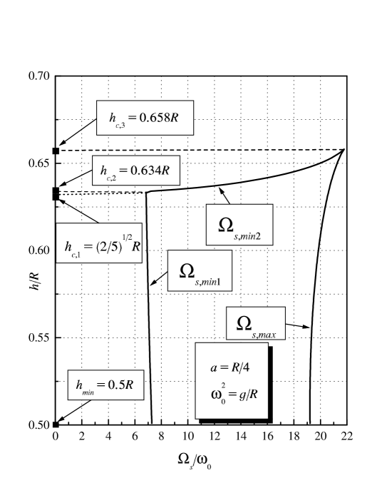
Figure 4: Boundaries of the stability region in the $\Omega_{s}$-$h$ plane.

Since each equilibrium height corresponds to a different repulsive magnetic force (and hence to a different mass) we can, alternatively, specify the allowed range of mass required for stable hovering by using Eq.8 and Eq.18 (note that the maximum height corresponds to the lightest mass and the minimum height corresponds to the heaviest mass). The results are plotted in Fig. 5.

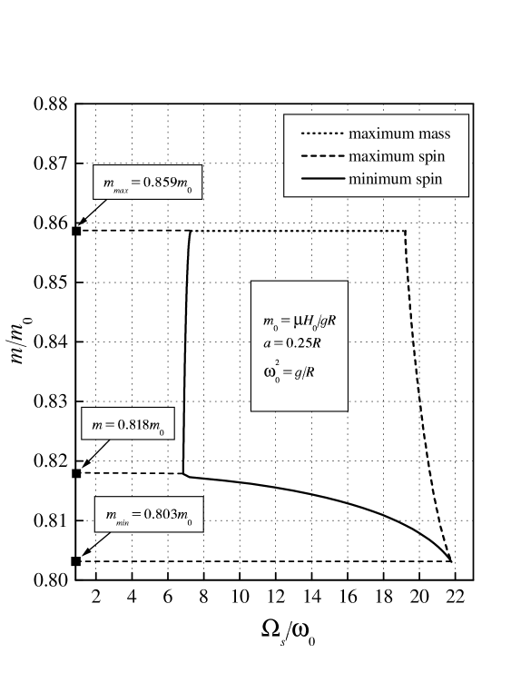
Figure 5: Boundaries of the stability region in the $\Omega_{s}$-$h$ plane.

From the figure we learn that, for $a=0.25R$, the mass of the top must be such that

$$0.803m_{0}\leq m\leq 0.859m_{0}$$

where

$$m_{0}\equiv\frac{\mu H_{0}}{gR}$$

This corresponds to a mass tolerance of

$$\frac{\Delta m}{m}\equiv 100\frac{m_{\mbox{max}}-m_{\mbox{min}}}{m_{\mbox{max}}}\simeq 7\%\mbox{.}$$ (19)

Experimentally the tolerance is only about $1\%$ which seems like a large discrepancy. Note, however, that the lower mass region (of less than $0.818m_{0}$) is difficult to access. Also, the top retains a finite kinetic energy when launched into the trap which, as has been discussed by us[13], further decreases the mass tolerance in practice. Last but not least, the theoretical mass tolerance, given in Eq.(19) decreases drastically with the tilt of the base, and goes to zero for a tilt of about $0.45$ degrees. This, in turn, makes it difficult to realize, in practice, the above theoretical mass tolerance, even with the leveling wedges supplied with the Levitron.

Note also that the temperature coefficient of the magnetization of the ceramic magnet from which the Levitron is made is about $0.2\%$ per degree Celsius. As the magnetic force varies with the square of the magnetization, temperature changes may easily ‘throw’ the mass out of range.

To overcome these problems the kit comes with a set of light washers to tune the mass properly.

4 Summary.

In this paper we have analyzed the hovering magnetic top while it is in mid-air without using any preliminary assumptions. To do this we expanded the magnetic field around the equilibrium point to second order in the spatial coordinates. Using the gradients of this field we then found the force and torque on the top and wrote down vectorial equations of motion for all 6 degrees of freedom. Next, we solved these equations analytically for the stationary solution and for a small perturbation around this stationary solution and arrived at a secular equation for the frequencies of the various possible modes. We then applied the solution to the case of a disk-like top hovering above a circular current loop, and were able to predict both the minimum and maximum allowed speeds for stable hovering to occur.

Although the numerical results we have presented in this paper refer to the case of a disk-like top ($I_{3}/I_{1}=2$), our theory is valid for the whole range of the anisotropy parameter $I_{3}/I_{1}$ of the symmetric top, and is therefore more general than the model studied in Ref.[8] who approximated the top by a classical spin. We recover their results by setting $I_{1}=0$ in our calculations[14]. Also, our analysis yields naturally the minimum spin for stability, which is zero for the $I_{1}=0$ case, and thus is put in ‘by hand’ in the previous [8] treatment. The determination of the maximum spin, as a function of the anisotropy parameter $I_{3}/I_{1}$, is of particular interest for cigar-like tops ($I_{3}/I_{1}<1$), as for such tops the minimum speed behaves drastically different than for disk-like tops ($2>I_{3}/I_{1}>1$), as we have shown elsewhere[15, 16].

An interesting corollary of our analysis is a limitation on the radius of the disk-like top. One would have expected that increasing the radius of the top will facilitate the operation of the Levitron as the moment of inertia increases, thus reducing the minimum speed. However, the maximum speed decreases faster when the radius increases, with the result that

$$\frac{\Omega_{s,\mbox{max}}}{\Omega_{s,\mbox{min}}}\simeq 0.66\frac{R}{r}.$$

Thus, the top cannot exceed two thirds of the base. Another detrimental effect of increasing the radius is the reduction of the hovering time[17] due to the increased effect of air friction. Moreover, air friction also modifies the stability analysis: So far we carried out a detailed study of the effect of friction on stability only for the $I_{1}=0$ model. In this case we found[16] that with friction the top is always unstable even if the friction is infinitesimaly small and even if we invoke translational viscosity only. We expect this behavior to occur also for $I_{1}\neq 0$ indicating that spin traps are different in character from potential traps in which friction ‘increases’ stability.

We have disregarded here the angular momentum carried by the electrons responsible for the ferromagnetic moment of the top. Although this is very small compared to the orbital angular momentum of the Levitron, the two angular momenta may become comparable for sufficiently small tops, which would result in a left-right asymmetry. Furthermore, the possibility of levitation based only on the electronic angular momentum arises. This will be discussed elsewhere[16].

Also, our treatment is completely classical. As size decreases, quantum-mechanical effects may become important. In particular, a sufficiently small particle, for example an atom, will only have a finite life-time in the trap due to quantum-mechanical effects, which will be considered elsewhere[16].

References

- [1] The Levitron is available from ‘Fascinations’, 18964 Des Moines Way South, Seattle, WA 98148.
- [2] Hones et al., U.S. Patent Number: 5,404,062, Date of Patent: Apr. 4, 1995.
- [3] The U-CAS is available from Masudaya International Inc., 6-4, Kuramae, 2-Chome, Taito-Ku, Tokyo, 111 Japan.
- [4] T. Bergeman, G. Erez, H. J. Metcalf, Phys. Rev. A., 35 (4), 1535-1546 (1987).
- [5] M. V. Berry, Proc. R. Soc. Lond. A 452, 1207-1220 (1996).
- [6] S. Gov and S. Shtrikman, Proc. of the 19 IEEE Conv. in Israel, 184-187 (1996).
- [7] S. Gov, H. Matzner and S. Shtrikman, Bulletin of the Israel Physical Society, 42, 121 (1996).
- [8] The same problem can also be treated by approximating the top by a classical spin. This is done by M. D. Simon, L. O. Heflinger and S. L. Ridgway, Am. J. Phys. 65 (4), 286-292 (1997).
- [9] “Vectorial Mechanics” by E. A. Milne, Methuen and Co. London, 322-323 (1948).
- [10] S. Earnshaw, Trans. Cambridge Philos. Soc. 7, 97-112 (1842).
- [11] “Classical Mechanics” by H. Goldstein, Addison-Wesley, 2 Ed., 213-225.
- [12] “Mechanics” by L. D. Landau and E. M. Lifshitz, Pergamon Press, 3 Ed., 111-114.
- [13] S. Gov, H. Matzner and S. Shtrikman, Bulletin of the Israel Physical Society, 43, 47 (1997).
- [14] setting is equivalent to approximating the top by classical spin. see for example “The Physical Principles of Magnetism” A. H. Morrish, John Wiley & Sons, pp. 551 (1965).
- [15] P. Flanders, S. Gov, S. Shtrikman and H. Thomas, Bulletin of the Israel Physical Society, 43, 44 (1997).
- [16] S. Gov, S Shtrikman and H. Thomas, to be published.
- [17] S. Gov, S. Shtrikman and S. Tozik, Bulletin of the Israel Physical Society, 42, 122 (1996).