Superluminal Optical Phase Conjugation: Pulse Reshaping and Instability

Abstract

We theoretically investigate the response of optical phase conjugators to incident probe pulses. In the stable (sub-threshold) operating regime of an optical phase conjugator it is possible to transmit probe pulses with a superluminally advanced peak, whereas conjugate reflection is always subluminal. In the unstable (above-threshold) regime, superluminal response occurs both in reflection and in transmission, at times preceding the onset of exponential growth due to the instability.

I Introduction

A variety of mechanisms is now known to give rise to superluminal (faster-than-$c$) group velocities, which express the peak advancement of electromagnetic pulses reshaped by material media:

1. Near-resonant absorption[1, 2]: anomalous dispersion in the linear regime of an absorbing medium forms the basis for this superluminal reshaping mechanism.

2. Reduced transmission or evanescent wave formation (tunneling) in passive dielectric structures[3, 4, 5]: this reshaping mechanism has been attributed to interference between multiply-reflected propagating pulse components in the structure[6].

3. Soliton propagation in dissipative nonlinear structures [7]: superluminal group velocities can occur in such systems via nonlinear three-wave exchanges, as in stimulated Brillouin backscattering in the presence of dissipation. They also occur in a nonlinear laser amplifier[8].

4. Pulse propagation in transparent (non-resonant) amplifying media[9, 10]. Superluminal pulse reshaping in this regime has been attributed to either the dispersion[9] or the boundary reflections[10] of the amplifying medium.

5. Tachyonic dispersion in inverted two-level media: the dispersion in such inverted collective systems is analogous to the tachyonic dispersion exhibited by a Klein-Gordon particle with imaginary mass[11]. Consequently, it has been suggested [12] that probe pulses in such media can exhibit superluminal group velocities provided they are spectrally narrow. Gain and loss have been assumed to be detrimental for such reshaping. We note that Ref. [12] describes an infinite medium and boundary effects on the reshaping have not been considered.

In this paper we establish a connection between optical phase conjugation and tachyonic-type behavior in a finite medium. To that end we study the reflection and transmission of pulses at a phase-conjugating mirror (PCM), both in its stable and in its unstable operating regimes. Similar features in other parametric processes, such as stimulated Raman scattering and parametric down-conversion will be treated elsewhere. The dispersion relation in infinite PCM media, which allows for superluminal group velocities, was derived by Lenstra[13]. Here we address the questions: can superluminal features be observed in the response of a finite PCM to an incident probe pulse, and how can they be reconciled with causality?

Pulse reshaping by a PCM has been studied before[14], but never in the context of superluminal behavior. We show (Sec. II B) that in the well-known stable operating regime of a PCM, superluminal peak advancement can occur in transmission but not in conjugate reflection, as was briefly presented in Ref. [15]. In the unstable regime (Sec. II C), we demonstrate the existence of superluminal peak advancement in both the reflected and transmitted wave response to spectrally narrow analytic probes. Further insight into these processes is gained by spatial wavepacket analysis (Sec. III). For sharply-timed (abruptly modulated, non-analytic) signals (Sec. IV) the occurrence of spectral components in the frequency zone where the gain is highest cannot be avoided. These components trigger early exponential growth, which is independent of the probe pulse shape. In all cases we develop criteria for the optimization of probe pulse shapes, aimed at maximizing their superluminal peak advancement and, in the unstable regime, the delay of the instability onset.

Our phase-conjugating mirror consists of a nonlinear optical medium with a large third-order susceptibility $\chi^{(3)}$, confined to a cell of length $L$. Phase conjugation is obtained through a four-wave mixing (FWM) process [16]: when the medium is pumped by two intense counterpropagating laser beams of frequency $\omega_{0}$ and a weak probe beam of frequency $\omega_{p}=\omega_{0}+\delta$ is incident on the cell, a fourth beam will be generated due to the nonlinear polarization of the medium. This conjugate wave propagates with frequency $\omega_{c}=\omega_{0}-\delta$ in the opposite direction as the probe beam (see Fig. 1).

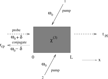
FIG. 1.: Phase conjugation by four-wave mixing. Solid (dashed, dotted) arrows denote pump (probe, conjugate) beams.

II Pulse reflection and transmission - temporal analysis

A Basic Analysis

The basic semiclassical one-dimensional equations describing this FWM process are obtained by substituting the total field $E(x,t)=\sum_{\alpha=1,2,p,c}E_{\alpha}(x,t)=\sum_{\alpha=1,2,p,c}{\cal E}_{\alpha}(x,t)e^{i(k_{\alpha}x-\omega_{\alpha}t)}+c.c.$ (where the labels 1,2 refer to the two pump beams and p,c to the probe and conjugate beams respectively) into the wave equation for a nonmagnetic, nondispersive material in the presence of a nonlinear polarization

$$\left(\frac{\partial^{2}}{\partial x^{2}}-\epsilon_{r}\epsilon_{0}\mu_{0}\frac{\partial^{2}}{\partial t^{2}}\right)E(x,t)=\frac{1}{\epsilon_{0}c^{2}}\frac{\partial^{2}}{\partial t^{2}}P_{NL}(x,t).$$ (1)

Selecting the phase-conjugation terms for $P_{NL}(x,t)=\chi^{(3)}E^{3}(x,t)$, assuming the pump beams to be non-depleted and applying the slowly varying envelope approximation (SVEA) results in[16]

$$\left(\begin{array}[]{cc}\frac{\partial}{\partial x}+\frac{1}{c}\frac{\partial}{\partial t}&i\,\kappa\vspace{0.3cm}\\ i\,\kappa^{*}&\frac{\partial}{\partial x}-\frac{1}{c}\frac{\partial}{\partial t}\end{array}\right)\left(\begin{array}[]{l}{\cal E}_{p}(x,t)\vspace{0.3cm}\\ {\cal E}_{c}^{*}(x,t)\end{array}\right)=0.$$ (2)

Here ${\cal E}_{p(c)}^{(*)}(x,t)$ denotes the complex amplitude of the probe (conjugate) field and $\kappa\equiv\kappa_{0}e^{i\phi}=\frac{3\omega_{0}}{\epsilon_{0}c}\chi^{(3)}{\cal E}_{1}{\cal E}_{2}$ is the coupling strength (per unit length) between the probe and conjugate wave. The dispersion relation for an electromagnetic excitation in this pumped nonlinear medium is given by [13]

$$k^{2}=\frac{\omega_{0}^{2}}{c^{2}}\pm\frac{2\omega_{0}}{c^{2}}\sqrt{\delta^{2}+\kappa_{0}^{2}c^{2}},$$ (3)

where $\delta=\omega_{p}-\omega_{0}=\omega_{0}-\omega_{c}$, and $k^{2}$ is the squared wavevector of both the probe and the conjugate waves.

The group velocity $\partial\delta/\partial k$ in the medium can be shown from (3) to be always larger than c, the speed of light in vacuum, and the dispersion relation is therefore of the tachyonic type (see Fig. 2(a)), analogous to the one for inverted atoms[12]. Because of the superluminal group velocity caused by this dispersion, the question arises how wave packets will be reshaped by a PCM. In the early 80’s, Fisher et al. studied the phase-conjugate reflection of pulses of arbitrary shape at a PCM[14]. No tachyonic effects were found. They distinguished between two different operating regimes of the mirror, stable (if $\kappa_{0}L<\frac{\pi}{2}$) and unstable (if $\kappa_{0}L>\frac{\pi}{2}$). In the stable regime, the response of the mirror is always finite and scales with the probe input. The unstable regime corresponds to self-generation of conjugate reflection from arbitrarily small probe input, followed by exponential growth until saturation is reached (due to depletion). Recently we predicted the occurrence of superluminal advancement of the peak of a suitably chosen input pulse upon transmission through a stable PCM[15]. Here we present the full analysis of both the stable and the unstable regimes and demonstrate the existence of superluminal effects in both.

In order to study pulse reflection and transmission at a PCM, we use the two-sided Laplace transform (TSLT) technique introduced by Fisher et al.[14]. The basic approach is summarized in App. A. To begin with, the reflection and transmission amplitudes for a monochromatic probe beam incident on a PCM are given by (Eqs. (A4) and (A5), at $x=0$ and $x=L$, respectively)

$$r_{cp}(\delta) = \frac{\kappa_{0}\sin(\beta L)}{\frac{\delta}{c}\mbox{\rm sin}(\beta L)+i\beta\mbox{\rm cos}(\beta L)}$$ (4)

$$t_{pp}(\delta) = \frac{i\beta}{\frac{\delta}{c}\mbox{\rm sin}(\beta L)+i\beta\mbox{\rm cos}(\beta L)}$$ (5)

where

$$\beta=\frac{1}{c}\sqrt{\delta^{2}+(\kappa_{0}\,c)^{2}}.$$ (6)

Now consider a probe field ${\cal E}_{p}(0,t)$ incident on the PCM at $x=0$, which satisfies the basic TSLT premise that it decreases faster than exponentially as $t\to-\infty$[17]. We obtain the expressions for the resulting reflected phase-conjugate pulse at $x=0$, and the transmitted probe pulse at $x=L$ from the inverse TSLT (see App. A). In taking the inverse TSLT we separate the singularities of $r_{cp}(is)$ and $t_{pp}(is)$ in the right-half $s$-plane, which give rise to unstable exponentially growing solutions, from the singularities in the left-half $s$-plane, which correspond to stable solutions. The final expressions for $0<\!\kappa_{0}\,\!L<\frac{3\pi}{2}$ are

$${\cal E}_{c}(0,t) = \frac{1}{2\pi i}\int_{-i\infty}^{i\infty}ds\,\bar{r}_{cp}(is)\,\tilde{{\cal E}}_{p^{*}}(0,s)\,e^{st}$$ (8)

$$+\ h_{1}\,\int_{-\infty}^{t}\,dt^{{}^{\prime}}\,{\cal E}_{p}^{*}(0,t^{{}^{\prime}})\,e^{-s_{1}(t^{{}^{\prime}}-t)},$$

$${\cal E}_{p}(L,t) = \frac{1}{2\pi i}\int_{-i\infty}^{i\infty}ds\,\bar{t}_{pp}(is)\,\tilde{{\cal E}}_{p}(0,s)\,e^{st}$$ (10)

$$+\ h_{2}\,\int_{-\infty}^{t}\,dt^{{}^{\prime}}\,{\cal E}_{p}(0,t^{{}^{\prime}})\,e^{-s_{1}(t^{{}^{\prime}}-t)}.$$

Here

$$\bar{r}_{cp}(is) \equiv r_{cp}(is)-\frac{h_{1}}{s-s_{1}}$$ (11)

$$\bar{t}_{pp}(is) \equiv t_{pp}(is)-\frac{h_{2}}{s-s_{1}}$$ (12)

$$s_{1} = \left|c\,\kappa_{0}\,\mbox{\rm cos}X_{1}\right|$$ (13)

$$h_{1} = -i\,c\,\kappa_{0}\,\mbox{\rm sin}^{2}(X_{1})/[1+\frac{Ls_{1}}{c}]$$ (14)

$$h_{2} = c\,X_{1}\,\mbox{\rm sin}(X_{1})/(L\,[1+\frac{Ls_{1}}{c}])$$ (15)

and $X_{1}$ the nontrivial solution of $\mbox{\rm sin}(X)=\pm X/(\kappa_{0}\,L)$. In the second terms in (8) and (10) $s_{1}$ is the unstable pole, and $h_{1}$ and $h_{2}$ are the residues of the reflection and transmission amplitudes at this pole. After rewriting the first term in (8) and (10) as a Fourier transform, it is straightforward to analyze ${\cal E}_{c}(0,t)$ and ${\cal E}_{p}(L,t)$ numerically. If $\kappa_{0}L\!<\!\pi/2$ there are no singularities with $\mbox{\rm Re}(s)>0$, so $h_{1}=h_{2}=0$ and the second term in (8) and (10) does not contribute. Hence, the stable regime is defined by $\kappa_{0}L<\pi/2$, and the unstable by $\kappa_{0}L>\pi/2$. We now start by studying pulse reshaping by a stable PCM, and then move on to the unstable regime.

B Stable regime

Fisher et al.[14] analyzed the phase-conjugate reflection at a PCM in the stable regime ($\kappa_{0}L<\pi/2$). For a gaussian input pulse they found a delay of the peak of ${\cal E}_{c}(0,t)$ with respect to that of ${\cal E}_{p}(0,t)$. Here we wish to emphasize that a suitably chosen incident pulse in this stable regime is reshaped in such a way that its peak emerges from the cell before the time it takes to travel the same distance in vacuum. The central result, obtained from Eqs. (8) and (10) with $h_{1}=h_{2}=0$, is depicted in Fig. 2(b).

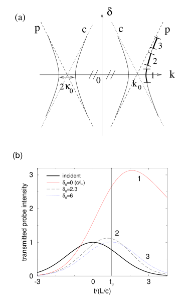
FIG. 2.: (a) Dispersion relation (solid line) in a PCM. The dashed (dotted) lines correspond to the dispersion relation for the probe (p) and conjugate (c) waves in vacuum and $k_{0}\equiv\omega_{0}/c$. The marked positions 1-3 indicate the frequency components in the incident pulses which give rise to the transmitted curves 1-3 in (b). (b) Transmitted probe pulse $|{\cal E}_{p}(L,t)|$ at $x=L$ for an incoming gaussian ${\cal E}_{p}(0,t)=e^{-\alpha t^{2}}e^{i\delta_{0}t}$ at $x=0$ (thick solid line). The temporal width (FWHM) of the incoming pulse $\Delta_{t}\equiv 2\sqrt{\ln 2/\alpha}=3.3\,L/c$, the spectral width $\Delta_{\delta}\equiv 4\sqrt{\alpha\ln 2}=1.7\,c/L$ and $\kappa_{0}L=1.4$. The vertical line indicates the time $t_{tr}=L/c$ needed to traverse the cell in vacuum.

The condition on the frequencies in the input signal for observing the superluminal effect is that they should be centered away from the gap in the dispersion relation. The reason for this is that a pulse which is centered around $\delta_{0}=0$ contains positive as well as negative frequency components whose respective positive and negative group velocities interact and compensate in such a way that no superluminal advancement occurs. For a pulse centered further up on the dispersion curve (Fig. 2(a)), however, superluminal peak advancement is obtained (at $\delta_{0}>2\,c/L$, curves 2 and 3 in Fig. 2(b)). This superluminal peak advancement depends on three parameters: the temporal width of the incoming pulse $\Delta_{t}$, the central frequency of the incoming pulse $\delta_{0}$ and the coupling strength in the medium $\kappa_{0}$. By fixing $\kappa_{0}$ and varying simultaneously $\Delta_{t}$ and $\delta_{0}$ the superluminal effect can be (numerically) optimized in several ways. In absolute terms, we find a maximal attainable peak advancement of $~{}\sim 0.88\,L/c$. But since this advancement, even though large, would only be a small effect if the pulse is broad in time, it is also useful to optimize the ratio $r=$ peak advancement/pulse width. We obtain a maximal relative peak advancement of $r\sim 0.08$. In phase-conjugate reflection no such superluminal effect appears: the time at which the peak of the reflected signal emerges at $x=0$ is always later than $t=0$, the time at which the maximum of the input pulse entered the cell.

C Unstable regime

We now move on to the unstable regime ($\kappa_{0}L>\pi/2$), for which Eqs. (8) and (10) have $h_{1},h_{2}\neq 0$. Figure 3 shows the reflected phase-conjugate pulse in this regime for an incident gaussian centered around frequency $\delta_{0}$.

FIG. 3.: Phase-conjugate reflected pulse $|{\cal E}_{c}(0,t)|$ at a PCM in its unstable operating regime ($\kappa_{0}L=1.7$) as a function of time (in units of $L/c$) for incident gaussian-shaped pulses ${\cal E}_{p}(0,t)=e^{-\alpha t^{2}}e^{i\delta_{0}t}$ with different $\delta_{0}$ (in units of $c/L$). Curves a, b and c correspond, respectively, to $\delta_{0}=0.1$, $0.28$ and $0.6$. $|{\cal E}_{p}(0,t)|$ (thick solid line) has temporal width $\Delta_{t}=2\sqrt{\ln 2/\alpha}=24\,L/c$ and spectral width $\Delta_{\delta}=4\sqrt{\alpha\ln 2}=0.23\,c/L$.

For $\delta_{0}=0.1\,c/L$ we see that the reflected signal starts growing exponentially as soon as the incoming pulse reaches the cell. However, for an incident pulse centered around a frequency further away from the gap in the dispersion relation (at $\delta_{0}\approx 0.28\,c/L$), the reflected pulse exhibits a local maximum before the exponential growth sets in. This peak is clearly advanced with respect to the peak of the incoming signal. Since $\kappa_{0}L$ is chosen close to $\pi/2$, the reflected pulse is greatly amplified[18].

For large $\delta_{0}$, where the dispersion relation becomes asymptotically linear ($\delta=\pm c(k_{0}\pm k)$), the reshaping of the reflected pulse is only minor and the superluminal effect is no longer noticeable for this pulse. In order to optimize the superluminal response preceding exponential growth, one must thus have $\delta_{0}$ small (for maximum advancement) and $\kappa_{0}L$ close to $\pi/2$ (for maximum intensity and delay of exponential growth).

Just as in the stable regime, we need to optimize three parameters simultaneously: $\kappa_{0}$, $\delta_{0}$ and $\Delta_{t}$. One way of doing this is by using the exact expression (8) and analyzing it numerically, but this does not give much insight into the interplay between these parameters. Another method is to find an approximation of the exact result, which allows for an analytical treatment of a certain class of incident pulses and yields quantitatively good agreement with the exact result in that case.

In order to obtain such an approximation we consider the conjugate reflection amplitude (4) in the limit $\delta\ll\kappa_{0}c$, corresponding to incident pulses with a large temporal bandwidth compared to $L/c$. Equation (4) then reduces to

$$r_{cp}(\delta)\approx\frac{\kappa_{0}c}{\delta+i/t_{m}}\hskip 17.07182pt\mbox{\rm for}\ \delta\ll\kappa_{0}c$$ (16)

with

$$t_{m}\equiv\frac{\mbox{\rm tan}(\kappa_{0}L)}{\kappa_{0}c}.$$ (17)

The reflected pulse becomes in this approximation

$${\cal E}_{c}(0,t)\approx-i\,\kappa_{0}\,c\,e^{-\frac{t}{t_{m}}}\,\int_{-\infty}^{t}dt^{{}^{\prime}}{\cal E}_{p}^{*}(0,t^{{}^{\prime}})e^{\frac{t^{{}^{\prime}}}{t_{m}}}$$ (18)

and we see that the growth in the unstable regime $t_{m}<0$ behaves as $e^{\frac{t}{|t_{m}|}}$. For spectrally narrow pulses and large $\kappa_{0}$, the difference between (18) and the exact numerical result is found to be $<10\%$.

Taking the derivative of $|{\cal E}_{c}(0,t)|$ from Eq. (18) with respect to $t$ and equating it to zero gives a condition on the times at which the reflected pulse is maximal ($t_{max}$) or minimal ($t_{min}$),

$$X^{2}(t)+Y^{2}(t)-t_{m}\,[X(t)X^{{}^{\prime}}(t)+Y(t)Y^{{}^{\prime}}(t)]=0,$$ (19)

with

$$X(t) = \int_{-\infty}^{t}dt^{{}^{\prime}}\mbox{\rm Re}({\cal E}_{p}^{*}(0,t^{{}^{\prime}}))e^{t^{{}^{\prime}}/t_{m}}$$ (20)

$$Y(t) = \int_{-\infty}^{t}dt^{{}^{\prime}}\mbox{\rm Im}({\cal E}_{p}^{*}(0,t^{{}^{\prime}}))e^{t^{{}^{\prime}}/t_{m}}.$$ (21)

The optimal superluminal effect is found if the reflected intensity is large at $t_{max}$ and close to zero at $t_{min}$ and the separation $t_{min}-t_{max}$ is as large as possible. In order to obtain the maximal relative advancement we numerically scan through the three-parameter space ($\kappa_{0}$, $\delta_{0}$, $\Delta_{t}$), fixing $\kappa_{0}L$ and varying the other two parameters simultaneously. Using (19), this reveals that the reflected pulse is very sensitive to $\delta_{0}$ (for fixed $\kappa_{0}$ and $\Delta_{t}$, see also Fig. 3) and only arises for incident pulses that are sufficiently broad in time ($\Delta_{t}\geq 20\,L/c$). For signals with broad spectra, the strong influence of frequency components in the instability gap prevents the formation of a discernible pulse response before exponential growth sets in. Furthermore, $\kappa_{0}L$ should be close to $\pi/2$, because otherwise the fast onset of exponential growth masks the reflected pulse. In the optimal case one can find an advancement of the peak of $t_{max}\sim 10\,L/c$ for a pulse of temporal width $\Delta_{t}\sim 25\,L/c$. The peak intensity $|{\cal E}_{c}(0,t_{max})|\sim 5$, $|{\cal E}_{c}(0,t_{min})|\sim 0.1$ and $t_{min}-t_{max}\sim 6\,L/c$.

The results for transmission of a gaussian through an active PCM are qualitatively the same as for phase-conjugate reflection. The amplitude of the advanced transmitted response is different, but not the values of $\delta_{0}$ and $\Delta_{t}$ for which it arises. The approximation (16) cannot be used to describe the transmission in the stable regime, which occurs for larger values of $\delta_{0}$ than the superluminal response in the unstable regime. The assumption $\delta\ll\kappa_{0}\,c$ is not valid in that case.

III Pulse reflection and transmission - spatial analysis

To gain further insight into pulse reshaping by a PCM, we follow an incoming gaussian pulse in space. One can then observe the following stages: (1) the probe wave packet approaches the cell; (2) it propagates as an ”optical quasiparticle” (consisting of a probelike part traveling to the right and a conjugatelike part traveling to the left)[19] in the cell and (3) the reflected phase-conjugate and transmitted probe packets leave the cell. We employ again the TSLT of Sec. II. The reflected phase-conjugate and transmitted probe pulses at position $x$ in the nonlinear medium and time $t$ are given by (App. A)

$${\cal E}_{c}^{\rm PCM}(x,t) = \frac{1}{2\pi i}\int_{\gamma-i\infty}^{\gamma+i\infty}ds\,h_{r}(x,is)\,\tilde{{\cal E}}_{p^{*}}(0,s)\,e^{st}$$ (22)

$${\cal E}_{p}^{\rm PCM}(x,t) = \frac{1}{2\pi i}\int_{\gamma-i\infty}^{\gamma+i\infty}ds\,h_{t}(x,is)\,\tilde{{\cal E}}_{p}(0,s)\,e^{st},$$ (23)

where $h_{r}(x,\delta)$ and $h_{t}(x,\delta)$ are given by Eqs. (A4) and (A5). For the setup of Fig. 1, the total probe pulse ${\cal E}_{p}(x,t)$ now consists of an incoming probe pulse in the region $x<0$, the probelike part of an ”optical quasiparticle” in the cell ($0<x<L$) and a transmitted probe pulse for $x>L$. The result is

$${\cal E}_{p}(x,t) = \theta(-x)\ {\cal E}_{p}^{\rm PCM}(0,t-\frac{x}{c})+$$ (26)

$$(\theta(x)-\theta(x-L))\ {\cal E}_{p}^{\rm PCM}(x,t)+$$

$$\theta(x-L)\ {\cal E}_{p}^{\rm PCM}(L,t-\frac{x-L}{c}),$$

where $\Theta$ is the Heaviside step function, and similarly,

$${\cal E}_{c}(x,t) = \theta(-x)\ {\cal E}_{c}^{\rm PCM}(0,t+\frac{x}{c})+$$ (28)

$$(\theta(x)-\theta(x-L))\ {\cal E}_{c}^{\rm PCM}(x,t).$$

We subtract from (26) and (28) again the contribution of the singularities which give rise to exponentially growing solutions, as in Eqs. (8) and (10), and rewrite them as Fourier integrals over frequency $\delta$. We then consider an incoming gaussian and analyze $|{\cal E}_{p}(x,t)|^{2}$ and $|{\cal E}_{c}(x,t)|^{2}$ as a function of x (and t) numerically, especially focusing on the intruiging pulse reshaping effects found before: the possibility for superluminal peak traversal times in probe transmission in the stable regime and the superluminal pulse response in the unstably operating PCM.

Figures 4 and 5 show the time evolution of a probe wave packet incident upon a PCM. The incoming pulse $|{\cal E}_{p}(x,t)|^{2}$ is centered around frequency $\delta_{0}$ and its width is given by (FWHM) $\Delta_{\delta}\equiv 2\,\sqrt{2\alpha\ln 2}$, which corresponds to a spatial width $\Delta_{x}=c\,\sqrt{2\ln 2/\alpha}$. For clarity $-|{\cal E}_{c}(x,t)|^{2}$ is plotted along the vertical axis instead of $+|{\cal E}_{c}(x,t)|^{2}$.

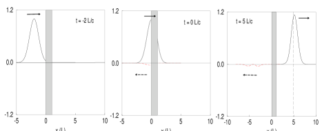
FIG. 4.: Stable regime (below-threshold) reflection and transmission of an incoming probe pulse at a PCM of length $L$ (indicated by shaded area). The solid (dashed) curve in the upper (lower) half of each time plot shows the probe (conjugate) pulse $|{\cal E}_{p}(x,t)|^{2}$ (- $|{\cal E}_{c}(x,t)|^{2}$), which is moving to the right (left). Parameters used are $\delta_{0}=3\,c/L$, $\Delta_{x}=2.1\,L$, $\Delta_{\delta}=1.3\,c/L$, $\kappa_{0}L=1.4$. The dashed vertical line for $t=5\,L/c$ indicates the position where the peak of the pulse would have been in the absence of the PCM.

Figure 4 depicts the probe transmission and conjugate reflection in the stable regime ($\kappa_{0}L<\pi/2$) for an incoming pulse of spatial width $2.1\,L$, centered around frequency $\delta_{0}=3\,c/L$ in the frequency domain. These parameters are comparable to those for curve 2 in Fig. 2, but since we now consider $|{\cal E}_{p}(x,t)|^{2}$ instead of $|{\cal E}_{p}(x,t)|$, the normalization is different. We see how the probe pulse approaches the cell at $t=-2\,L/c$. At $t=0$, when the forward tail of the pulse has entered the cell, a small reflected phase-conjugate pulse has developed and is traveling simultaneously in the opposite direction. At $t=5\,L/c$ the advancement of the transmitted probe peak is clearly visible: the position of the peak is $x_{peak}\approx 6\,L$, whereas it would have been $5\,L$ if the pulse had propagated through vacuum (see dashed vertical line in the figure).

In the unstable regime, for $\kappa_{0}L>\pi/2$, the instability leads to enormous growth of $|{\cal E}_{p}(x,t)|^{2}$ and $|{\cal E}_{c}(x,t)|^{2}$ as the probe pulse enters the cell. For a spectrally narrow pulse centered around $\delta_{0}=0$, exponential growth sets in immediately for that part of the probe which has reached the cell boundary at $x=0$. For an incoming pulse centered around $\delta_{0}\sim 0.3\,c/L$ the ”transient” behavior is recovered. This is illustrated in Fig. 5: at $t=0$ the growth of the incoming signal has set in in the PCM, but in addition there is a clear phase-conjugate pulse with a superluminally advanced peak traveling to the left. At the same time one sees a superluminal ”kink” in the transmitted probe response: the instability prevents the formation of a full gaussian-shaped transmitted probe pulse for this set of parameters. The $t=10\,L/c$ time plot shows the superluminally reflected signal on a larger scale.

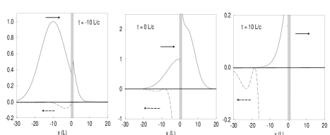
FIG. 5.: Unstable (above-threshold) regime of the PCM: reflection and transmission of an incoming probe pulse. The PCM is located between $0<x<L$ (see shaded area). The upper (lower) half of each time plot shows the probe (conjugate) pulse $|{\cal E}_{p}(x,t)|^{2}$ (- $|{\cal E}_{c}(x,t)|^{2}$), which is moving to the right (left). Parameters used are $\delta_{0}=0.31\,c/L$, $\Delta_{x}=19.3\,L$, $\Delta_{\delta}=0.144\,c/L$, $\kappa_{0}L=1.7$.

IV Chopped signals

Analytic gaussians are of little value as far as information transfer is concerned, or as a check whether the observed superluminal effects are in agreement with causality[6, 9, 20]. For that purpose, one needs an incoming modulated or chopped signal. Interesting questions then arise: how is the sudden change in the input pulse reflected in the output pulse? How are the reflected response and exponential growth in the unstable regime affected by this change? We have already shown elsewhere that for probe transmission in the stable regime, the edge of a chopped incoming signal is always transmitted causally[15]. Figure 6 shows the transmitted probe response in the unstable regime for an incident gaussian pulse which is suddenly switched off at $t=0$.

FIG. 6.: Transmitted probe pulse $|{\cal E}_{p}(L,t)|$ through a PCM at $x=L$ for an incident gaussian-shaped chopped pulse (thick solid line). Curves a and b correspond to $\delta_{0}=0.28$ and $0.3$ respectively. The parameters used are the same as in Fig. 3 and $t_{tr}$ indicates the time it takes to traverse the cell in vacuum.

We see that the sudden change in the incoming pulse is carried over into the transmitted probe response at time $t_{tr}\equiv L/c$, the time it takes to traverse the cell in vacuum. The ”information content” of the pulse is thus transmitted with the speed of light, after which the exponential growth due to the instability immediately sets in. Note that the superluminal peak advancement of the reflected conjugate pulse remains, just as for the full gaussian of Fig. 3. This advancement does not violate causality, but is a pulse reshaping effect. The fact that the chopped edge of the pulse is transmitted with the speed of light can be seen more clearly by expressing ${\cal E}_{p}(x,t)$ as (App. A)

$${\cal E}_{p}(L,t)=\sum_{n=0}^{\infty}\int_{-\infty}^{t-(n+\frac{1}{2})\tau}dt^{{}^{\prime}}{\cal E}_{p}(0,t^{{}^{\prime}})\,L_{n}(t,t^{{}^{\prime}}),$$ (29)

with

$$\begin{array}[]{rl}L_{n}(t,t^{{}^{\prime}})&=\frac{\kappa_{0}c}{2}A_{n}^{-\frac{1}{2}}\left(A_{n}^{n}I_{2n-1}\left[\kappa_{0}c\,\sqrt{(t-t^{{}^{\prime}})^{2}-(n+\frac{1}{2})^{2}\tau^{2}}\,\right]\right.\vspace{0.2cm}\\ &-2A_{n}^{n+1}I_{2n+1}\left[\kappa_{0}c\,\sqrt{(t-t^{{}^{\prime}})^{2}-(n+\frac{1}{2})^{2}\tau^{2}}\,\right]\vspace{0.2cm}\\ &\left.+A_{n}^{n+2}I_{2n+3}\left[\kappa_{0}c\,\sqrt{(t-t^{{}^{\prime}})^{2}-(n+\frac{1}{2})^{2}\tau^{2}}\,\right]\ \ \right),\end{array}$$ (30)

and

$$A_{n}\equiv\left(\frac{t-t^{{}^{\prime}}-(n+\frac{1}{2})\tau}{t-t^{{}^{\prime}}+(n+\frac{1}{2})\tau}\right)^{1/2}.$$ (31)

Here $I_{n}$ are the modified Bessel functions. ${\cal E}_{p}(L,t)$ is now expressed as a sum of integrals, in which the $n^{th}$ term corresponds to the contribution after the $n^{th}$ round-trip time $\tau=2\,L/c$. The advantage of this expression is that it shows that for an incoming chopped signal, which is suddenly switched on at $t=t_{0}$, the transmitted response only starts at $t=t_{0}+L/c$, in agreement with causality.

V Conclusions

In conclusion, we have theoretically studied the reflection and transmission of wave packets at a phase-conjugating mirror. Our main findings are

(a) In the stable operating regime (for $\kappa_{0}L<\pi/2$), the peak of the transmitted signal can exhibit a superluminal peak-traversal time[15]. The conditions for this effect are that the incoming analytic probe signal be spectrally narrow and centered around a frequency sufficiently far away from the parametric resonance ($\delta=0$ in Fig. 2(a)). The maximum advancement obtained is $\sim 0.88\,L/c$ and the maximum ratio (peak advancement)/(pulse width) $\sim 0.08$. No such effect is found in the reflected phase-conjugate response, whose peak is always delayed with respect to the one of the incoming probe signal (Sec. II B). The salient advantage of superluminal peak transmission in this stable regime is that the output pulse is undistorted.

(b) In the unstable regime (for $\kappa_{0}L>\pi/2$), for incident probe pulses with a temporal width much larger than $L/c$, a pronounced ”transient” reflected phase-conjugate response develops before the onset of exponential growth due to the instability. This pulse response exhibits a superluminally advanced peak, both in phase-conjugate reflection and in probe transmission (Sec. II C). The advancement and intensity are maximal for $\kappa_{0}L$ close to $\pi/2$ and the response is very sensitive to the central frequency $\delta_{0}$ of the incoming pulse.

(c) We have demonstrated (Sec. IV) that the superluminal features are observable only for temporally broad analytic pulses, in agreement with the principle of causality, whereas a sudden (non-analytic) change in the incident probe pulse propagates with the speed of light.

Finally, the question arises how these pulse reshaping effects can be observed. For a realistic PCM, consisting of a cell of length $L\sim 10^{-2}$ m, coupling strengths of $\kappa_{0}c\sim c/L\sim 10^{10}s^{-1}$ have been reached, so that tan${}^{2}(\kappa_{0}L)\sim 1$[22]. In order to observe pulse reshaping in the stable operating regime of this PCM, one needs an incident probe pulse of width $\sim 0.1$ ns whose peak is then transmitted with a superluminal peak transmission time $\sim 0.01$ ns. To enter the unstable regime, the PCM has to be operated using pulsed pump beams. The pump pulses should be long enough to allow for observation of the ”transient” pulse response, but short enough to avoid the instability effects. Since the width of the superluminally reflected and transmitted response is on the order of $\sim 10\,L/c$, nanosecond pump-pulse durations are required.

A Two-sided Laplace transform technique

In this appendix we briefly outline the two-sided Laplace transform (TSLT) technique introduced by Fisher et al.[14]. The TSLT is defined as $\tilde{\cal F}_{(*)}(x,s)\equiv\int_{-\infty}^{\infty}dt\,F^{(*)}(x,t)\,e^{-st}$. It is only valid for functions $F(x,t)$ that diminish faster than exponentially at times $t\to-\infty$[17]. Its advantage compared to the the usual one-sided Laplace transform is that it also applies to functions that do not vanish at $t<0$. The starting point of the analysis is to apply the TSLT to the four-wave mixing equations (2) with $F(x,t)={\cal E}_{p}(x,t)$ or ${\cal E}_{c}^{*}(x,t)$. We then obtain the coupled equations

$$\left\{\begin{array}[]{l}\frac{d}{dx}\,\tilde{\cal E}_{p}(x,s)+\frac{s}{c}\,\tilde{\cal E}_{p}(x,s)+i\kappa\,\tilde{\cal E}_{c,*}(x,s)=0\vspace{0.3cm}\\ \frac{d}{dx}\,\tilde{\cal E}_{c,*}(x,s)-\frac{s}{c}\,\tilde{\cal E}_{c,*}(x,s)+i\kappa^{*}\,\tilde{\cal E}_{p}(x,s)=0.\end{array}\right.$$ (A1)

Equations (A1) are solved together with the Laplace transforms of the boundary conditions ${\cal E}_{p}(0,t)=F(0,t)$, where $F(0,t)$ is an incident probe pulse at the entry $x=0$ of the PCM medium, and ${\cal E}_{c}(L,t)=0$, so no incoming conjugate pulse at the end of the medium. The result is

$$\tilde{\cal E}_{c}(x,s) = h_{r}(x,is)\,\tilde{\cal F}_{*}(0,s)$$ (A2)

$$\tilde{\cal E}_{p}(x,s) = h_{t}(x,is)\,\tilde{\cal F}(0,s),$$ (A3)

with the reflection and transmission amplitudes

$$h_{r}(x,\delta) = \frac{\kappa_{0}\sin(\beta(L-x))}{\frac{\delta}{c}\mbox{\rm sin}(\beta L)+i\beta\mbox{\rm cos}(\beta L)}\vspace{0.3cm}$$ (A4)

$$h_{t}(x,\delta) = \frac{i\beta\cos(\beta(L-x))+\frac{\delta}{c}\sin(\beta(L-x))}{\frac{\delta}{c}\mbox{\rm sin}(\beta L)+i\beta\mbox{\rm cos}(\beta L)},$$ (A5)

where $\beta$ is given by Eq. (6).

The reflected phase-conjugate pulse ${\cal E}_{c}(x,t)$ and transmitted probe pulse ${\cal E}_{p}(x,t)$ at position $x$ in the nonlinear medium and time $t$ are then obtained by using the inverse Laplace transform. At $x=0$ and $x=L$, respectively, they are given by

$${\cal E}_{c}(0,t) = \frac{1}{2\pi i}\int_{\gamma-i\infty}^{\gamma+i\infty}ds\,r_{cp}(is)\,\tilde{{\cal E}}_{p^{*}}(0,s)\,e^{st}$$ (A6)

$${\cal E}_{p}(L,t) = \frac{1}{2\pi i}\int_{\gamma-i\infty}^{\gamma+i\infty}ds\,t_{pp}(is)\,\tilde{{\cal E}}_{p}(0,s)\,e^{st},$$ (A7)

where $r_{cp}=h_{r}(x=0)$ and $t_{pp}=h_{t}(x=L)$. The choice of contour $\gamma$ in (A6) and (A7) is in agreement with causality, which means in this case that it is to the right of all the singularities of $r_{cp}(is)$ (and $t_{pp}(is)$). The singularities in the right-half s-plane give rise to exponential growth of ${\cal E}_{c}(x,t)$ and ${\cal E}_{p}(x,t)$. The integrals (A6) and (A7) can be evaluated by taking the contribution of these poles separately and rewriting the remaining integral as a Fourier integral, see (8) and (10).

They can also be evaluated in another way, which is especially insightful when regarding non-analytic, chopped probe pulses (Sec. IV). To that end we rewrite (A6) and (A7) as

$${\cal E}_{c}(0,t) = \int dt^{{}^{\prime}}\,{\cal E}_{p}^{*}(0,t^{{}^{\prime}})H_{c}(t,t^{{}^{\prime}})$$ (A8)

$${\cal E}_{p}(L,t) = \int dt^{{}^{\prime}}\,{\cal E}_{p}(0,t^{{}^{\prime}})H_{p}(t,t^{{}^{\prime}}),$$ (A9)

with

$$H_{c}(t,t^{{}^{\prime}}) = \frac{1}{2\pi i}\int_{\gamma-i\infty}^{\gamma+i\infty}ds\,r_{cp}(is)\,e^{-s(t^{{}^{\prime}}-t)}$$ (A10)

$$H_{p}(t,t^{{}^{\prime}}) = \frac{1}{2\pi i}\int_{\gamma-i\infty}^{\gamma+i\infty}ds\,t_{pp}(is)\,e^{-s(t^{{}^{\prime}}-t)}$$ (A11)

In order to evaluate the integral in, e.g., $H_{p}(t,t^{{}^{\prime}})$, $t_{pp}$ is first rewritten as the series

$$t_{pp}(is)=2\eta\sum_{n=0}^{\infty}\frac{a^{2n}}{(s+\eta)^{2n+1}}\,e^{-(n+\frac{1}{2})\eta\tau}$$ (A12)

with $a\equiv\kappa_{0}c$, $\eta\equiv\sqrt{s^{2}-a^{2}}$ and $\tau=2L/c$, the roundtrip time of the PCM. One can then easily prove that (A12) is uniformly convergent, which allows for term by term integration of (A11). We use the substitution

$$s=\frac{ia}{2}\left(\frac{u}{A_{n}}-\frac{A_{n}}{u}\right)$$ (A13)

with

$$A_{n}\equiv\left(\frac{t-t^{{}^{\prime}}-(n+\frac{1}{2})\tau}{t-t^{{}^{\prime}}+(n+\frac{1}{2})\tau}\right)^{1/2},$$ (A14)

in which $t^{{}^{\prime}}+(n+\frac{1}{2})\tau$ is the retardation time after $(n+\frac{1}{2})$ round trips. We then arrive at the result Eq. (29).

Similarly, the conjugate reflected pulse is given by

$${\cal E}_{c}(L,t) = \int_{-\infty}^{t}dt^{{}^{\prime}}\,{\cal E}_{p}^{*}(0,t^{{}^{\prime}})\,M_{0}(t,t^{{}^{\prime}})+$$ (A16)

$$-2\sum_{n=1}^{\infty}\int_{-\infty}^{t-n\tau}dt^{{}^{\prime}}{\cal E}_{p}^{*}(0,t^{{}^{\prime}})\,M_{n}(t,t^{{}^{\prime}}),$$

with

$$\begin{array}[]{rl}M_{n}(t,t^{{}^{\prime}})&=\frac{-i\,\kappa_{0}c}{4}\left(B_{n}^{n-1}I_{2n-2}\left[\kappa_{0}c\,\sqrt{(t-t^{{}^{\prime}})^{2}-n^{2}\tau^{2}}\,\right]\right.\vspace{0.2cm}\\ &-2B_{n}^{n}I_{2n}\left[\kappa_{0}c\,\sqrt{(t-t^{{}^{\prime}})^{2}-n^{2}\tau^{2}}\,\right]\vspace{0.2cm}\\ &\left.+B_{n}^{n+1}I_{2n+2}\left[\kappa_{0}c\,\sqrt{(t-t^{{}^{\prime}})^{2}-n^{2}\tau^{2}}\,\right]\ \ \right),\end{array}$$ (A17)

and

$$B_{n}\equiv\left(\frac{t-t^{{}^{\prime}}-n\,\tau}{t-t^{{}^{\prime}}+n\,\tau}\right).$$ (A18)

REFERENCES

- [1] L. Brillouin, Wave Propagation and Group Velocity, (Academic Press, New York, 1960).
- [2] C.G.B. Garrett and D.E. McCumber, Phys. Rev. A 1, 305 (1970); S. Chu and S. Wong, Phys. Rev. Lett. 48, 738 (1982).
- [3] M. Büttiker and R. Landauer, Phys. Rev. Lett. 49, 1739 (1982); Th. Martin and R. Landauer, Phys. Rev. A 45, 2611 (1992).
- [4] A. M. Steinberg, P.G. Kwiat, and R.Y. Chiao, Phys. Rev. Lett. 68, 2421 (1992).
- [5] A. Ranfagni, D. Mugnai, and A. Agresti, Phys. Lett. A 175, 334 (1993). 1089 (1993).
- [6] Y. Japha and G. Kurizki, Phys. Rev. A 53, 586 (1996).
- [7] E. Picholle, C. Montes, C. Leycuras, O. Legrand, and J. Botineau, Phys. Rev. Lett. 66, 1454 (1991).
- [8] A. Icsevgi and W.E. Lamb, Phys. Rev. 185, 517 (1969).
- [9] E. L. Bolda, Phys. Rev. A 54, 3514 (1996); E. L. Bolda, J.C. Garrison, and R.Y. Chiao, ibid 49, 2938 (1994).
- [10] M. Artoni and R. Loudon, Phys. Rev. A 57, 622 (1998).
- [11] Y. Aharonov, A. Komar, and L. Susskind, Phys. Rev. 182, 1400 (1969).
- [12] R.Y. Chiao, A.E. Kozhekin, and G. Kurizki, Phys. Rev. Lett. 77, 1254 (1996).
- [13] D. Lenstra, in Huygens Principle 1690-1990; Theory and Applications, edited by H. Blok, H.A. Ferwerda, and H.K. Kuiken (North Holland, Amsterdam, 1990).
- [14] R.A. Fisher, B.R. Suydam, and B.J. Feldman, Phys. Rev A 23, 3071 (1981).
- [15] M. Blaauboer, A.E. Kozhekin, A.G. Kofman, G. Kurizki, D. Lenstra, and A. Lodder, Opt. Comm. 148, 295 (1998).
- [16] Optical Phase Conjugation, edited by R.A. Fisher (Academic Press, New York, 1983).
- [17] G. Doetsch Theorie und Anwendung der Laplace-Transformation, (Dover, New York, 1943).
- [18] If the intensities of probe and conjugate waves approach those of the two pumps, pump depletion has to be taken into account and our analysis is not valid anymore.
- [19] The name ”optical quasiparticles” is introduced in view of the analogy[13, 21] with the quasiparticle excitations in a superconductor, described by the Bogoliubov-de Gennes equations, see P.G. de Gennes, Superconductivity of Metals and Alloys, (Benjamin, New York, 1966). Just as these superconductor quasiparticles have a mixed electron-hole character, the optical quasiparticles consist of both a probe and a conjugate part.
- [20] R.Y. Chiao, A.M. Steinberg, and P.G. Kwiat in Quantum Interferometry, edited by F. de Martini, G. Denardo, and A. Zeilinger (World Scientific, Singapore, 1994).
- [21] H. van Houten en C.W.J. Beenakker, Physica B 175, 187 (1991).
- [22] M.Y. Lanzerotti, R.W. Schirmer, and A.L. Gaeta, Appl. Phys. Lett 69, 1199 (1996).