Diagnostic criterion for crystallized beams

Abstract

Small ion crystals in a Paul trap are stable even in the absence of laser cooling. Based on this theoretically and experimentally well–established fact we propose the following diagnostic criterion for establishing the presence of a crystallized beam: Absence of heating following the shut–down of all cooling devices. The validity of the criterion is checked with the help of detailed numerical simulations.

The production of crystallized beams is the holy grail of storage ring physics [1, 2]. As a matter of fact crystallization has already been achieved in a miniature storage ring with essentially stationary ions [3]. Crystallization in high energy storage rings, however, remains an elusive goal although many laboratories throughout the world are working on the problem (see, e.g., [4, 5, 6, 7]). Apart from electron cooling [8], laser cooling [9, 10] is now employed by some groups [4, 5, 6, 7] as the most efficient and most promising method to achieve the low beam temperatures required for beam crystallization. Judging from the enormous progress achieved in the past few years success seems imminent. But while it is straightforward to observe ion crystals in traps [11] directly with the help of CCD cameras [12, 13, 14, 15, 16], it is very difficult to observe the internal structure of a fast beam in a storage ring directly with optical means. As a matter of fact, no such observation has been reported so far. Other imaging methods may require structural changes of existing storage rings which are both technically difficult and costly. In view of these difficulties it becomes imperative to devise diagnostic tools different from direct optical observation that are capable of distinguishing between a crystallized and a non-crystallized beam. It is the purpose of this paper to suggest a simple diagnostic criterion capable of making this distinction. The criterion is based on a hysteresis effect first described experimentally in connection with ion crystals in a Paul trap [13]. It is rooted in the observation that once an ion crystal has been produced, e.g., by laser cooling, it remains stable even in the absence of laser cooling [16]. Since in the center–of–mass frame the ion beam in a storage ring has similar physics to that of ions in a Paul trap, we suggest to use absence of heating as a diagnostic criterion for the crystalline state of an ion beam in a storage ring.

Before proceeding to the analytical and numerical treatment of absence of heating, let us introduce an intuitive picture using the classical phase space of the ion beam. Due to the interplay between the (effectively time–dependent) confining forces and the Coulomb interaction between ions the dynamics of the ions is in general chaotic, resulting in energy diffusion. Nevertheless, the crystalline state and its vicinity correspond to a region in phase space in which the dynamics is linear and thus regular. Hence, if linearly stable, this region can be described as a regular island in phase space [17, 18, 19] in which the trajectories are dynamically trapped. As a consequence, the time–averaged gain in energy or action is zero. This is equivalent with the absence of heating. Because of the possibility of dynamic trapping of phase–space trajectories in regular islands, it is now clear on physical grounds why ion crystals can survive even in the absence of a cooling mechanism. We call these crystals stable. Thus, we formulate the following diagnostic criterion for beam crystallization: A beam in a storage ring is crystallized if no heating occurs following the shut–down of all cooling devices. Our criterion works for stable crystals. It is important to emphasize that the simplest possible ion crystal in a storage ring, the linear chain [20, 21], is of this type if the density is low (see discussion below). It is equally important to emphasize the possibility of unstable crystals for which our criterion does not work. The phase–space trajectory of an unstable crystal is linearly unstable near the crystalline state in the absence of cooling. A crystalline state may nevertheless exist if the cooling is strong enough to overcome the dynamical instability. The resulting crystal is called unstable since in the absence of cooling the linear instability leads to heating and melting of the crystal. In this paper we focus our attention exclusively on the physics of stable crystals deferring discussion of unstable crystals to a separate publication [22].

In the remainder of this paper we discuss the physics, the validity and the limits of applicability of the proposed beam–crystallization criterion. We illustrate the discussion with the results of numerical simulations of a model that captures the essence of the physics of crystallization of very low density beams. The model consists of $N$ ions subject to the time–dependent Hamiltonian

$$H=K+V_{\rm int}+V_{\rm conf}$$ (1)

where

$$K=\sum_{i=1}^{N}\frac{\vec{P}_{i}^{2}}{2m}$$ (2)

is the kinetic energy,

$$V_{\rm int}=\sum_{1\leq j<i\leq N}\frac{{\cal Z}^{2}e^{2}}{4\pi\epsilon_{0}}\frac{1}{\left|\vec{R_{i}}-\vec{R_{j}}\right|}$$ (3)

is the Coulomb interaction potential, and

$$V_{\rm conf}=\sum_{i=1}^{N}\left[\Phi_{0}\cos(\Omega t)(X_{i}^{2}-Y_{i}^{2})-\Psi_{0}(X_{i}^{2}+Y_{i}^{2}-2Z_{i}^{2})\right]$$ (4)

is the confining potential. Here $\vec{R}_{i}=(X_{i},Y_{i},Z_{i})$ are the Cartesian coordinates of the $i$th ion in the rest frame of the beam, $\vec{P}_{i}$ are its momenta, $m$ denotes the mass of the ions, ${\cal Z}e$ is their charge, $\Omega$ is the frequency of the confining fields as seen from the rest frame of the moving ion and $\Phi_{0}$, $\Psi_{0}$ are positive constant parameters. The coordinate system is oriented such that the $Z$ axis corresponds to the beam axis and the $X,Y$ plane is orthogonal to the beam. The confining potential $V_{\rm conf}$ contains a dynamic (time dependent) strongly focusing part in the transverse $X,Y$ directions that models the action of the quadrupole focusing magnets, and a bucket–like static part that models the bunching along the beam direction ($Z$-axis). The similarity of (1)–(4) to the Hamiltonian of an $N$ particle Paul trap is apparent. It allows us to draw useful analogies from the well–developed field of ion traps. The time–dependent part of the confining potential $V_{\rm conf}$ gives rise to the micromotion [23] of the beam particles. Away from the crystalline configuration the micromotion results in fast heating of the beam, a phenomenon that is completely analogous to the radio–frequency (rf) heating of ion clouds in a Paul trap [23].

The equations of motion derived from (1) can be conveniently scaled and are given by:

$$\ddot{x_{i}} = -\gamma_{x}\dot{x_{i}}+\lambda_{0}\sum_{j\neq i,j=1}^{N}\frac{(x_{i}-x_{j})}{\left|\vec{r_{i}}-\vec{r_{j}}\right|^{3}}+\left[a-2q\cos(2\tau)\right]x_{i}\;,$$ (5)

$$\ddot{y_{i}} = -\gamma_{y}\dot{y_{i}}+\lambda_{0}\sum_{j\neq i,j=1}^{N}\frac{(y_{i}-y_{j})}{\left|\vec{r_{i}}-\vec{r_{j}}\right|^{3}}+\left[a+2q\cos(2\tau)\right]y_{i}\;,$$ (6)

$$\ddot{z_{i}} = -\gamma_{z}\dot{z_{i}}+\lambda_{0}\sum_{j\neq i,j=1}^{N}\frac{(z_{i}-z_{j})}{\left|\vec{r_{i}}-\vec{r_{j}}\right|^{3}}-2az_{i}\;,$$ (7)

where we used the following definitions:

$$\Omega t\equiv 2\tau\;,\;\;\vec{R}_{i}\equiv l_{0}\vec{r}_{i}\;,\;\;\lambda_{0}\equiv\frac{{\cal Z}^{2}e^{2}}{\pi\epsilon_{0}m\Omega^{2}l_{0}^{3}}\;,\;\;a\equiv\frac{8\Psi_{0}}{m\Omega^{2}}\;,\;\;2q\equiv\frac{8\Phi_{0}}{m\Omega^{2}}.$$ (8)

In the above equations we added a (possibly anisotropic) damping effected by the damping constants $\gamma_{x}$, $\gamma_{y}$, $\gamma_{z}$ to model the laser cooling.

In our computations we model $N=5$ ions of ²⁴Mg⁺ with $q=0.2$ and $a=q^{2}/64$. The external frequency $\Omega$ is $2\pi\times 3$ MHz and the length scale $l_{0}$ is chosen to be 1 $\mu$m. The damping serves as our control parameter. With this choice of parameters the typical spatial extension of the ion ensemble in $z$ direction is about four times the extension in the $x,y$ directions. In other words, our parameters are chosen such that the ions experience a focusing force that is about four times stronger in the $x,y$ directions compared to the $z$ direction. For this choice of parameters the linear chain is the lowest energy crystalline configuration of our model system [20, 21]. The integration of the equations of motion (5)–(7) was performed using a variable–order, variable–step Adams method [24].

Although our model of five ions seems like a caricature of a real beam in a storage ring, it captures the essence of cooling and crystallization of low-density beams in strongly focusing machines. An indication to this effect is the following observation. When we simulated anisotropic cooling, i.e., $\gamma_{x}=\gamma_{y}=0$, $\gamma_{z}=\gamma>0$, we faced the same problem as the experiments: with anisotropic cooling it is very difficult to create Coulomb crystals with reasonable choices of $\gamma$. Moreover, we think of our model as describing a typical section of the beam rather than a system consisting of a small number of ions. This is substantiated by the fact that near the linear crystal state essentially only the nearest neighbor Coulomb interactions are important, since the Coulomb force reduces like the square of the distance. Hence the number of total ions is not of primary importance. We note that the static confining potential is suitable for bunched beams, while periodic boundary conditions that preserve linear density are suitable for coasting beams. We emphasize that our calculations are microscopic and do not suffer from any further approximations beyond the choice of the model Hamiltonian (1).

In order to keep things as simple as possible, and since the applicability of our crystallization criterion does not depend on the type of cooling scheme used to produce a crystallized beam, we illustrate the criterion and the physics of beam crystallization with the help of isotropic cooling, i.e. $\gamma_{x}=\gamma_{y}=\gamma_{z}=\gamma>0$.

Many of our numerical results reported below are discussed within the framework of ion temperature $T$. The temperature here is only a convenient way of expressing the experimentally measured mean–square of the ion velocity. We follow the convention used by the experimentalists and use the standard thermodynamic relation $\langle(\dot{\vec{R}}-\langle\dot{\vec{R}}\rangle)^{2}\rangle\equiv 3k_{\rm B}T/m$, where $\langle\cdots\rangle$ denote averaging over ions. We thus avoid all questions of the thermodynamic relevance of defining a temperature for five particles as well as the question of how to define a temperature in the presence of a strong coherent drive.

Before embarking on the central point of diagnosing the crystal state, we present some relevant results relating to the cooling and crystallization process itself. We show that, depending on the cooling strength $\gamma$, an initially prepared generic hot ion cloud [15, 16] evolves according to three qualitatively different scenarios. In figure 1 we show the temperatures of our five ion ensemble as a function of (scaled) time $\tau$, and for three different values of $\gamma$. Curve (a) shows the temperature for $\gamma=10^{-4}$. The temperature decays exponentially ($\sim\exp(-\gamma\tau)$) right from the beginning of the simulation. This is the strong damping regime. Curve (b) of figure 1 shows a qualitatively different behavior for an intermediate choice of the cooling strength $\gamma=7\times 10^{-6}$. The beam is in the state of a hot cloud over a substantial period of time (much longer than $1/\gamma$). It collapses suddenly (at an exponential rate) to zero temperature from some time on. This behavior is called intermittent [25]. Curve (c) of figure 1, for $\gamma=10^{-6}$, shows a hot beam which remains hot over the total time interval of our simulations ($\tau_{\rm max}=10^{8}=100/\gamma$) although the cooling is constantly switched on. In this case the cooling is balanced by the rf heating. The heating is due to Coulomb collisions (intra-beam scattering) in the presence of the time–dependent fields in (1). This mechanism is also active in ion traps [26] and has been identified as the dominant heating mechanism in storage ring beams [4]. In both the weak and the intermediate cooling regimes the end result of the simulations, i.e., the zero temperature state, is the linear chain. This is illustrated in figure 2. It shows the $z$-coordinates of our five-ion ensemble corresponding to curve (b) of figure 1. After a chaotic transient lasting for about $0\leq\tau\leq 6\times 10^{6}$ we see a sudden crystallization of the five ions into stationary positions approximately equi-spaced on the $z$ axis. Inspection of the $x$ and $y$ coordinates shows $x_{i}\approx 0$, $y_{i}\approx 0$. Thus, the crystalline state corresponds to a linear chain. In our simulations, as seen from figure 2, the spacing of the ions is $\Delta_{z}\approx 30\mu$m. The linear chain is the natural crystalline configuration for very low density crystalline beams. It does not suffer from the problem of shear heating [2], a serious obstacle on the way to three-dimensionally crystallized beams in presently existing accelerator storage rings. Thus, establishing the linear chain is an important corner stone on the way to more complicated crystal configurations. Chaotic transients similar to the one shown in figure 1 were described earlier by Hoffnagle and Brewer [25] in connection with the two-ion Paul trap.

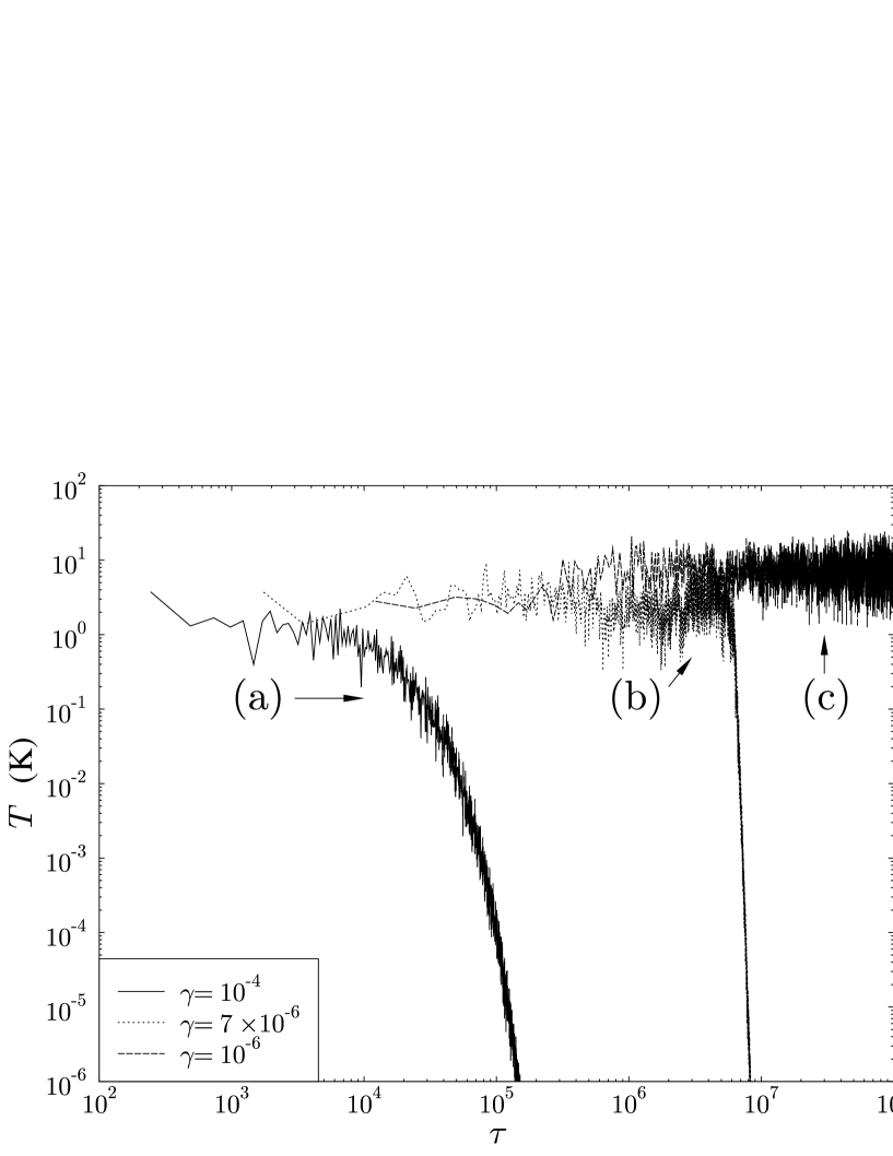
FIG. 1.: Three different scenarios for the time evolution of an initially hot state (cloud) of ions: (a) Immediate crystallization ($\gamma=10^{-4}$, strong damping regime), (b) intermittency ($\gamma=7\times 10^{-6}$, intermediate damping regime) and (c) persistent cloud ($\gamma=10^{-6}$, weak damping regime).

FIG. 2.: Time dependence of the $z$ coordinates of the five ions of the intermittent case (b) of figure 1. The ions crystallize out of a transiently chaotic state at $\tau\approx 6.5\times 10^{6}$ and arrange themselves regularly spaced in a crystallized linear chain. The lattice spacing in the crystalline state is $\Delta_{z}\approx 30\mu$m.

The statistical significance of the results shown in figures 1 and 2 is substantiated in figure 3. It gives a global view of the cooling process by showing the final beam temperatures after $\tau_{\rm max}=100/\gamma$ for a wide range of $\gamma$ values and a few initial conditions each. It shows also the temperatures in the cloud state in the intermittent cases. We observe that for small cooling power the beam remains in a hot state over the entire observation time $0\leq\tau\leq\tau_{\rm max}$. The temperature of the hot state decreases with increasing cooling strength. For strong cooling, crystallization takes place immediately. For intermediate cooling power there is intermittency, but the overall transition from a cloud to a crystal state is sharp as a function of $\gamma$.

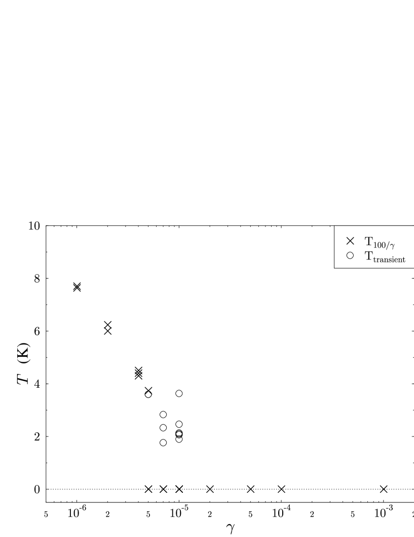
FIG. 3.: Beam temperatures as a function of cooling strength $\gamma$. Crosses: Final beam temperatures after a run time of $\tau=100/\gamma$. Circles: Beam temperature shortly before the onset of the sharp crystallization transition in the intermittent regime.

We now turn to the key point of this paper: The absence of heating of ion crystals. Absence of heating serves as a simple diagnostic tool for the crystalline state of ion beams. We shall focus here exclusively on linear crystals. In order to demonstrate the absence of heating, we picked three different initial conditions of the ion beam close to the linear crystalline state and integrated the equations of motion with the damping switched off ($\gamma=0$). In figure 4 we plot the resulting temperatures as a function of the time for three representative cases, in which the initial temperatures were $6.7\times 10^{-3}$ K, $6.7\times 10^{-2}$ K and $6.7\times 10^{-1}$ K. The integration was carried out over the time interval $0\leq\tau\leq 10^{7}$ which corresponds to $\approx 3\times 10^{6}$ cycles of the focusing force. For the two cases at lower temperature, we clearly observe the absence of heating. This means that even when there is no cooling, the beam remains very close to the linear crystalline state for a very long time. As expected, when the initial temperature is large enough (about 1 K in our case) the crystal melts quickly due to rf heating and the temperature increases dramatically. After an initial fast “blow–up” phase the heating continues on a slower scale. The initial blow–up shown in figure 4 strongly resembles the beam blow-up shown in [5] after switch–off of the electron cooler. From figure 4 we conclude that if the linear crystal is cold enough, then it can maintain itself even if the cooling power is switched off.

FIG. 4.: Time dependence of beam temperatures for three different initial conditions close to the crystalline configuration with no cooling $(\gamma=0)$. Upper curve: Initial temperature is $6.7\times 10^{-1}$ K, middle curve: Initial temperature is $6.7\times 10^{-2}$ K, lower curve: Initial temperature is $6.7\times 10^{-3}$ K. The upper curve shows strong heating. It does not correspond to a crystalline state. The two cases with lower initial temperatures show absence of heating. They correspond to a crystallized beam according to the proposed diagnostic criterion.

A few comments are in order now. First, as discussed above, our criterion fails to identify unstable crystals. Second, especially if the cooling process is rapid, we may produce a disordered, “glassy” state without geometric order that may be stable in the absence of cooling. Thus our criterion would wrongly identify a glass as a crystal. In general, therefore, applying the strictest standards, our criterion is neither necessary nor sufficient for the proper identification of geometrically ordered crystalline states. However if we restrict ourselves to low–density ion beams, which is the current experimental trend, then we are in much better shape. Indeed, if the ion density is small enough, the beam will crystallize to a linear chain, which excludes glassy states. This is substantiated by the work of Hasse and Schiffer [21] and by the work of Habs [20] as well as by our numerical simulations. Quantitatively it requires $\lambda\equiv\lambda_{0}/\Delta_{z}^{3}\lesssim 1$. Moreover, a detailed analytical investigation which we carried out and will appear elsewhere [22] indicates that the linear crystal is stable in the absence of cooling, provided that in the two-dimensional parameter space of the Mathieu equation the interval $([a,a+4.21\lambda],q)$ is contained in a stable region. This is the case if $\Delta_{z}$ is large enough, i.e., for very low density beams. Hence the above analysis indicates that for small values of the parameter $\lambda$ our no-heating criterion is both necessary and sufficient for the identification of a linear crystal. Let us note that in our simulations $\lambda\approx 2\times 10^{-3}$. Indeed, we never encountered a glassy state and our linear crystal was stable even without cooling in full agreement with the above discussion.

In practice our diagnostic criterion may be applied according to the following three steps:

1. We start with a hot beam.

2. The cooling devices are switched on (e.g. electron and/or laser cooling) resulting in a cold beam whose state (crystal or not) is to be determined.

3. All cooling devices are switched off.

If the beam is indeed crystallized, no heating will be observed. The beam remains crystallized. If the beam is just cold, but not crystallized, heating is observed after shut–down of the cooling devices. We emphasize that the shut-down should occur slowly, not abruptly. This is because in our simulations we noticed that a sudden switch–off of the damping results in a phase–jump in the time dependence of the ion trajectories leading to instantaneous heating of the system that may be strong enough to disrupt the crystalline state. However, there is no problem if the shut–down is slow on the scale of the micromotion of the beam particles.

A last comment concerns the beam observation time scale after shut–down of the cooling devices. It is clear that even if the beam was crystallized, it will heat slowly due to, e.g. fluctuations in the confining fields and the ambient thermal radiation. When we talk about heating after shut–down of the cooling devices we mean the fast rf heating due to the time–dependent confining fields in (1). Since the noise processes are much slower than rf heating, there should be no problem to separate the two mechanisms experimentally.

To summarize, in this paper we proposed a beam diagnostic criterion for deciding whether an ion beam in a storage ring is crystallized or not. The criterion is simple to apply and does not require any technical installations that are not already present in existing storage rings. With the help of model calculations we demonstrated that the criterion works well for low–density crystallized ion chains. The criterion has a limited range of validity, but since we expect that the first crystalline geometry achieved in a storage ring will be the linear chain, the crystallization criterion may play an important role in proving experimentally the presence of a crystallized beam in a storage ring.

The authors acknowledge fruitful discussions with R. Grimm and with M. Weidemüller. H. P. is grateful for a MINERVA postdoctoral scholarship. R. B. is grateful for financial support by the Deutsche Forschungsgemeinschaft (SFB 276).

REFERENCES

- [1] J. P. Schiffer and P. Kienle, Z. Phys. A 321, 181 (1985).
- [2] A. Rahman and J. P. Schiffer, Phys. Rev. Lett. 57, 1133 (1986).
- [3] G. Brikl, S. Kassner and H. Walther, Europhys. News 23, 143 (1992).
- [4] D. Habs and R. Grimm, Ann. Rev. Nucl. Part. Sci. 45, 391 (1995).
- [5] H.-J. Miesner, R. Grimm, M. Grieser, D. Habs, D. Schwalm, B. Wanner, and A. Wolf, Phys. Rev. Lett. 77, 623 (1996).
- [6] J. S. Hangst, M. Kristensen, J. S. Nielsen, O. Poulsen, J. P. Schiffer, P. Shi, Phys. Rev. Lett. 67, 1238 (1991).
- [7] J. S. Hangst, J. S. Nielsen, O. Poulsen, P. Shi, and J. P. Schiffer, Phys. Rev. Lett. 74, 4432 (1995).
- [8] H. Danared, Physica Scripta T59, 121 (1995).
- [9] T. W. Hänsch and A. L. Schawlow, Opt. Commun. 13, 68 (1975).
- [10] S. Stenholm, Rev. Mod. Phys 58, 699 (1986).
- [11] P. K. Ghosh, Ion Traps (Clarendon Press, Oxford, 1995).
- [12] J. Hoffnagle, R. G. DeVoe, L. Reyna, and R. G. Brewer, Phys. Rev. Lett. 61, 255 (1988).
- [13] F. Diedrich, E. Peik, J. M. Chen, W. Quint and H. Walther, Phys. Rev. Lett. 59, 2931 (1987).
- [14] D. J. Wineland, J. C. Bergquist, W. M. Itano, J. J. Bollinger, and C. H. Manney, Phys. Rev. Lett. 59, 2935 (1987).
- [15] R. Blümel, J. M. Chen, E. Peik, W. Quint, W. Schleich, Y. R. Shen and H. Walther, Nature 334, 309 (1988).
- [16] R. Blümel, C. Kappler, W. Quint, and H. Walther, Phys. Rev. A 40, 808 (1989).
- [17] E. Ott, Chaos in Dynamical Systems, (Cambridge University Press, Cambridge, 1993).
- [18] J. Guckenheimer and P. Holmes, Nonlinear Oscillations, Dynamical Systems and Bifurcations of Vector Fields, (Springer, New York, 1983).
- [19] A. J. Lichtenberg and M. A. Lieberman, Regular and Stochastic Motion, (Springer, New York, 1983).
- [20] D. Habs, in Frontiers of particle beams, Lecture notes in Physics 296, ed. M. Month and S. Turner, (Springer, New-York, 1988).
- [21] R. W. Hasse and J. P. Schiffer, Ann. Phyc. 203, 419 (1990)
- [22] H. Primack and R. Blümel, in preparation.
- [23] H. Dehmelt, Adv. At. Mol. Phys. 3, 53 (1967).
- [24] NAG Fortran Library Manual, Mark 14, The Numerical Algorithm Group Limited, Oxford, England, 1990.
- [25] J. Hoffnagle and R. G. Brewer, Phys. Rev. A 50, 4157 (1994).
- [26] R. G. Brewer, J. Hoffnagle, R. G. DeVoe, L. Reyna, and W. Henshaw, Nature (London) 344, 305 (1990).