On the evaluation of some three-body variational integrals

Abstract

Stable recurrence relations are presented for the numerical computation of the Calais-Löwdin integrals

$$\int\text{d}{\bf r}_{1}\text{d}{\bf r}_{2}\,r_{1}^{l-1}r_{2}^{m-1}r_{12}^{n-1}\,\exp{\{-\alpha r_{1}-\beta r_{2}-\gamma r_{12}\}}$$

($l$, $m$ and $n$ integer, $\alpha$, $\beta$ and $\gamma$ real) when the indices $l$, $m$ or $n$ are negative. Useful formulas are given for particular values of the parameters $\alpha$, $\beta$ and $\gamma$.

I Introduction

When dealing with the three-body variational problem with Hylleraas basis, it is usually necessary to make extensive use of integrals of the general form [1]

$$I(l,m,n;\,\alpha,\beta,\gamma)=\frac{1}{16\pi^{2}}\int\text{d}{\bf r}_{1}\text{d}{\bf r}_{2}\,r_{1}^{l-1}r_{2}^{m-1}r_{12}^{n-1}\,\exp{\{-\alpha r_{1}-\beta r_{2}-\gamma r_{12}\}}\,,$$ (1)

where $r_{1}=\left|{\bf r}_{1}\right|$, $r_{2}=\left|{\bf r}_{2}\right|$ and $r_{12}=\left|{{\bf r}_{2}-{\bf r}_{1}}\right|$.

For the case of $l$, $m$ and $n$ non-negative (that is, non-negative powers of $r_{1}$, $r_{2}$ and $r_{12}$ once the volume element has been taken into account), powerful, simple and stable recurrence relations that permit the numerical calculation of these integrals can be found in the literature [2]. However, it is sometimes essential to have also an expression for one of the integer indices being negative. For instance, that happens in the atomic problem when one wants to consider the mean value of the $r_{12}^{-2}$ operator [3] or relativistic corrections [4]; or in the nuclear problem when non-local terms are included in a Yukawa-like interaction [5]. In some cases, the integrals must be computed in every step of the non-linear optimization procedure, and hence it is clear the need of having a quick and reliable algorithm to compute them. The specific cases $I(1,1,-1)$ and $I(0,-1,-1)$ were already considered in Refs. [3] and [6] respectively. For $\gamma=0$ much work has been done [2, 7, 8, 9, 10, 11], also including explicitly the coupling of the angular momentum of the two dynamical particles [12]. Some work has been devoted to the analogous integrals for four- or more-body problems [6, 7, 11, 13, 14].

The method proposed in this work to obtain the integrals (1) is specially useful when the same exponential coefficients $\alpha$, $\beta$ and $\gamma$ appear in several elements of the variational basis.

II General properties of $\textstyle I(l,m,n)$

To study the general properties of the integral (1) for $l$, $m$ and $n$ (possibly negative) integer numbers and $\alpha$, $\beta$ and $\gamma$ real it is convenient to make use of perimetric coordinates [15],

$$\left.\begin{array}[c]{lcr}u&=&-r_{1}+r_{2}+r_{12}\\ v&=&r_{1}-r_{2}+r_{12}\\ w&=&r_{1}+r_{2}-r_{12}\\ \end{array}\right\}$$ (2)

in terms of which the initial integral reads

$$I(l,m,n;\,\alpha,\beta,\gamma)=2^{-(l+m+n+3)}\,I_{p}\left(l,m,n;\frac{\beta+\gamma}{2},\frac{\alpha+\gamma}{2},\frac{\alpha+\beta}{2}\right)\,,$$ (3)

where

$$I_{p}(l,m,n;\,a,b,c)=\int_{0}^{\infty}\text{d}u\int_{0}^{\infty}\text{d}v\int_{0}^{\infty}\text{d}w\,(v+w)^{l}(u+w)^{m}(u+v)^{n}\,\exp{\{-au-bv-cw\}}\,.$$ (4)

The integral $I_{p}$ is explicitly invariant under permutation of conjugated pairs of parameters $\{(l,a),(m,b),(n,c)\}$, and therefore

$$I(l,m,n;\,\alpha,\beta,\gamma)=I(m,l,n;\,\beta,\alpha,\gamma)=I(n,m,l;\,\gamma,\beta,\alpha)\,,$$ (5)

symmetry that will be used throughout this work.

The long range convergence of $I_{p}$ is ensured if $a$, $b$ and $c$ are positive real numbers, that is, if

$$\alpha+\beta>0\,,\quad\alpha+\gamma>0\quad\text{and}\quad\beta+\gamma>0\,.$$ (6)

That means that one of the exponentials parameters, $\alpha$, $\beta$ or $\gamma$, can be zero or negative, provided that the other two are bigger than the absolute value of the former. Note also that one of the exponential coefficients of $I_{p}$ can be zero if the power of the corresponding integration variable is negative and high enough. For instance, $a=0$ with $l=0$ and $m=n=-1$ would yield a convergent result. Anyhow, this is an almost useless case for the variational problem, because for higher power integrals (that very likely should also be considered) $a=0$ would lead to divergent quantities. From now on, we assume that the requirements (6) are fulfilled.

The study of the short range convergence can be straightforwardly done case by case. Summarizing, for $l$, $m$ and $n$ integer, and $\alpha$, $\beta$ and $\gamma$ real such that the conditions (6) are fulfilled, the integral (1) is convergent if and only if

$$l\geq-1\,,\quad m\geq-1\,,\quad n\geq-1\quad\text{and}\quad l+m+n\geq-2\,.$$ (7)

To have a procedure to generate the whole set of integrals (1) one needs relations for the cases $I(l,m,-1)$ and $I(l,-1,-1)$ where $l$ and $m$ are non-negative.

As soon as we have checked that the integral we are looking for is convergent, integration over one parameter can be applied to lower the conjugated power,

$$I(l,m,n;\,\alpha,\beta,\gamma)=\int_{\gamma}^{\infty}\text{d}c\,I(l,m,n+1;\,\alpha,\beta,c)\,.$$ (8)

On the other hand, derivation can always be used to increase indices,

$$(-\partial_{\alpha})^{p}I(l,m,n;\alpha,\beta,\gamma)=I(l+p,m,n;\alpha,\beta,\gamma)\,.$$ (9)

These properties, together with

$$I(0,0,0;\alpha,\beta,\gamma)=(\alpha+\beta)^{-1}(\alpha+\gamma)^{-1}(\beta+\gamma)^{-1}\,,$$ (10)

are useful to derive all the integrals. Note also that for $\lambda>0$

$$I(l,m,n;\lambda\alpha,\lambda\beta,\lambda\gamma)=\lambda^{-(l+m+n+3)}I(l,m,n;\alpha,\beta,\gamma)\,,$$ (11)

that is, for given $l$, $m$ and $n$, $I$ is a homogeneous function of $\alpha$, $\beta$ and $\gamma$. This fact, together with properties (5) and (9) yields a quite general recursion. Indeed, differentiating with respect to $\lambda$ in the equation above one gets the recurrence relation

$$(l+m+n+3)I(l,m,n;\alpha,\beta,\gamma) = \alpha I(l+1,m,n;\alpha,\beta,\gamma)+\beta I(l,m+1,n;\alpha,\beta,\gamma)$$ (13)

$${}+\gamma I(l,m,n+1;\alpha,\beta,\gamma)\,,$$

valid for well defined integrals, in our case $l$, $m$ and $n$ fulfilling conditions (7). In general, this recursion is of little utility, for to use it downwards, which is the obvious direction, one would have to know the value of the integrals on a plane $l+m+n=\text{constant}$. We will take profit of a particular case of Eq. (13) in section IV.

III Case $\textstyle I(l,m,-1)$ with $\textstyle l,m\geq 0$

For the family of integrals $I(l,m,-1;\alpha,\beta,\gamma)$ with $l,m\geq 0$, a variation of the method exposed in Ref.[2] can be applied. The recurrence relation that one gets is the following,

$$I(l,m,-1;\alpha,\beta,\gamma)=\frac{1}{\alpha+\beta}\left[lI(l-1,m,-1)+mI(l,m-1,-1)+B(l,m)\right]\,,$$ (14)

where

$$B(l,m;\alpha,\beta,\gamma)=l!\,m!\,\int_{\gamma}^{\infty}\text{d}c\,(\alpha+c)^{-l-1}\,(\beta+c)^{-m-1}\,,$$ (15)

which is a symmetric function under $(l,\alpha)\leftrightarrow(m,\beta)$ exchange, can be obtained through the relation

$$B(l,m)=\frac{1}{\alpha-\beta}\left[lB(l-1,m)-mB(l,m-1)+C(l,m)\right]\,.$$ (16)

Here the function $C(l,m)$ reads

$$C(l,m;\alpha,\beta,\gamma)=\left\{\begin{array}[]{ll}(m-1)!\,(\beta+\gamma)^{-m}&\quad\text{if}\quad l=0\quad\text{and}\quad m>0\\ -(l-1)!\,(\alpha+\gamma)^{-l}&\quad\text{if}\quad l>0\quad\text{and}\quad m=0\\ \log{(\alpha+\gamma)\over(\beta+\gamma)}&\quad\text{if}\quad l=0\quad\text{and}\quad m=0\\ 0&\quad\text{otherwise}\end{array}\right.$$ (17)

and is defined so that the recursion (16) holds also for $l=m=0$ although $B(0,-1)$ and $B(-1,0)$ are divergent. Note that $C(l,m)$ is antisymmetric under $(l,\alpha)\leftrightarrow(m,\beta)$.

Unfortunately, in the recursion (16) subtractions are involved, and hence one must look over the stability against roundoff, in particular when $\alpha$ and $\beta$ are close to each other.

It is also possible to relate $B(l,m)$ to Gauss hypergeometric function, ${}_{2}F_{1}$ [16], yielding

$$B(l,m;\alpha,\beta,\gamma)=\frac{l!\,m!}{m+l+1}\,(\alpha+\gamma)^{-l-1}\,(\beta+\gamma)^{-m}\,{}_{2}F_{1}(1,l+1;m+l+2;z)\,,$$ (18)

where $z\equiv\frac{\alpha-\beta}{\alpha+\gamma}$. The use of the integral representation of the hypergeometric function gives

$$B(l,m;\alpha,\beta,\gamma)=(l+m)!\,(\alpha+\gamma)^{-l-1}\,(\beta+\gamma)^{-m}\,\int_{0}^{1}{\rm d}t\,\frac{t^{l}\,(1-t)^{m}}{1-zt}\,.$$ (19)

From the definition (15) it is possible to prove the equation

$$B(l+1,m)+B(l,m+1)=l!\,m!\,(\alpha+\gamma)^{-(l+1)}\,(\beta+\gamma)^{-(m+1)}\qquad(l,m\geq 0)\,.$$ (20)

Plugging this relation in Eq. (16) yields

$$(l+m)\,B(l-1,m)-(\alpha-\beta)\,B(l,m)-(l-1)!\,m!\,(\alpha+\gamma)^{-l}\,(\beta+\gamma)^{-m}=0\,,$$ (21)

valid for $m\geq 0$ and $l>0$. This equation permits to lower one unit the index $l$ of $B(l,m)$ with numerical stability if $\alpha>\beta$. In the opposite case, the symmetry of $B(l,m)$ can be used to lower the index $m$ (see Fig. 1).

On the other hand, using the Gauss relations for contiguous hypergeometric functions one obtains

$$m\,B(l+1,m-1)+(m-l\,\xi)\,B(l,m)-l\,\xi\,B(l-1,m+1)=0\,,$$ (22)

where $\xi\equiv 1-z=\frac{\beta+\gamma}{\alpha+\gamma}$. This relation defines a recursion that can be used to move on the diagonals $m+l=\,\text{constant}$. As it is shown in Fig. 1, the straight line $m(l)=\xi\,l$ on the $l$-$m$-plane separates the stability regions of the recursion (22), so that one can move with stability from this line in diagonal steps.

The final recipe to compute the set of $I(l,m,-1;\alpha,\beta,\gamma)$ for $l,m\leq N$ is the following (see Fig. 1). First, two $B$’s are to be computed numerically to the required accuracy, namely

$$B\left(\left[\frac{2N}{1+\xi}\right],2N-\left[\frac{2N}{1+\xi}\right]\right)\text{ and }B\left(\left[\frac{2N}{1+\xi}\right]+1,2N-\left[\frac{2N}{1+\xi}\right]-1\right)$$ (23)

(respectively, points $P_{1}$ and $P_{2}$ in Fig. 1). Then the recursion (22) is used to generate all needed starting points to use the recursion (21) leftwards (downwards) if $\alpha>\beta$ ($\alpha<\beta$). Finally, the $B$’s obtained in this way are introduced in Eq. (14). To generate the two initial $B$’s one can compute the integral in Eq. (19) by Gauss-Legendre quadrature. To optimize the computation of the quadrature a change of variable is needed. First, we use the symmetry of $B(l,m)$ to render $0\leq z<1$. Next, we apply in Eq. (19) the change of variable ($t\to s=s(t)$)

$$s(t)=\left\{\begin{array}[]{cl}t&\quad\text{if}\quad 0\phantom{.0}\leq z<0.8\\ \log{(2-z-t)}&\quad\text{if}\quad 0.8\leq z\leq 0.99\\ \end{array}\right.$$ (24)

For values of $z$ greater than 0.99 the hypergeometric function can be computed using the transformation formula 15.3.11 of the Ref. [16]. With the prescription above, more than fifteen stable figures were obtained using 32 Gauss-Legendre points for $2N\leq 60$. Note that the prescription (24) has been optimized for the computation of the two initial $B$’s given in the expression (23), and will not provide a similar accuracy for arbitrary values of $l$ and $m$.

The particular case $\alpha=\beta$ is specially simple. Indeed, in that case the $B$ function to be included in Eq. (14) is

$$B(l,m;\alpha,\alpha,\gamma)=\frac{l!m!}{l+m+1}(\alpha+\gamma)^{-(l+m+1)}\,,$$ (25)

and the calculations are numerically stable. The case $\alpha=\beta$ is not only a mere academic example. In many practical problems the variational basis is chosen so that any element has the same exponential coefficient both for the coordinates $r_{1}$ and $r_{2}$. If the physical problem requires to deal with $I(l,m,-1)$ integrals, then it is sensible to check whether such a basis can produce the required accuracy. This selection was successfully used in the context of a nuclear theory problem [5].

In Table I we give some particular values of $I(l,m,-1;\alpha,\beta,\gamma)$ with fourteen significant figures to provide the reader with checking points.

IV Case $\textstyle I(l,-1,-1)$ with $\textstyle l\geq 0$

To generate the set of integrals $I(l,-1,-1)$ use can be made of the relation

$$\alpha\,I(l+1,-1,-1;\alpha,\beta,\gamma) = (l+1)I(l,-1,-1;\alpha,\beta,\gamma)$$ (27)

$${}-\beta I(l,0,-1;\alpha,\beta,\gamma)-\gamma I(l,-1,0;\alpha,\beta,\gamma)\,,$$

which is valid for $l\geq 0$. This equation is easily obtained as a particular case of recurrence (13). For $l=0$ direct calculation yields

$$I(0,-1,-1;\alpha,\beta,\gamma)=\frac{1}{2\alpha}\left[\frac{\pi^{2}}{6}-\log{\frac{\alpha+\gamma}{\beta+\gamma}}\log{\frac{\alpha+\beta}{\beta+\gamma}}-\text{Li}_{2}\left(\frac{\beta-\alpha}{\beta+\gamma}\right)-\text{Li}_{2}\left(\frac{\gamma-\alpha}{\beta+\gamma}\right)\right]$$ (28)

(see also Ref. [6]), where $\text{Li}_{2}(z)=-\int_{0}^{z}\rm{d}y\,y^{-1}\log(1-y)$ is the dilogarithm function.

As said, the expression (13) is not applicable for the case $l=m=n=-1$. Instead, one gets

$$\alpha I(0,-1,-1;\alpha,\beta,\gamma)+\beta I(-1,0,-1;\alpha,\beta,\gamma)+\gamma I(-1,-1,0;\alpha,\beta,\gamma)=\frac{\pi^{2}}{4}\,.$$ (29)

To fix the constant in the right hand side, we had to make explicit use of the expression (28).

The recursion (27), which in general is numerically unstable upwards, can be used with stability to decrease the index $l$ if $\alpha>0$, which is the interesting case in physics. But then, one needs as starting point the integral with the highest wanted $l$. As it can be derived from Eqs. (8-10), that integral can be obtained through the computation of the quadrature

$$I(l,-1,-1;\alpha,\beta,\gamma)=\frac{l!}{2}\,\left(\frac{2}{\beta+\gamma}\right)^{l+1}\,\int_{0}^{1}{\rm d}t\,\frac{1}{t}\,G_{l}\left(\frac{2\alpha}{\beta+\gamma},\frac{2\beta}{\beta+\gamma};\frac{1}{t}\right)\,,$$ (30)

where we have defined

$$G_{l}(a,b;y) = \frac{1}{(a+y)^{l+1}}\left\{\log\frac{(a+b+2(y-1))(a-b+2y)}{(a+b)(a-b+2)}\right.\phantom{aaaaaaaaaaaaaaaaaaaaaaaa}$$ (32)

$$\left.+\sum_{m=1}^{l}\frac{1}{m}\left[\left(\frac{a+y}{a+b}\right)^{m}+\left(\frac{a+y}{a-b+2}\right)^{m}-\left(\frac{a+y}{a-b+2y}\right)^{m}-\left(\frac{a+y}{a+b+2(y-1)}\right)^{m}\right]\right\}\,.$$

Note that the integrand is positive, and that the sum in the function $G_{l}$ is very efficiently computed in a single loop. For values of $\alpha$, $\beta$ and $\gamma$ of the same order of magnitude the quadrature converges very quickly for not very small values of $l$ ($l>5$). This is not the case when one of the parameters is larger than the other, but then a simple change of variable helps to recover convergence. For instance, the following prescription of changes of variable ($t\to s=s(t)$)

$$s(t)=\left\{\begin{array}[]{cl}\log{\left(t+\frac{\beta+\gamma}{2\alpha}\right)}&\quad\text{if}\quad\alpha>\frac{l}{10}(\beta+\gamma)\\ \log{\left(1+\frac{\alpha+\min\{\beta,\gamma\}}{2(\beta+\gamma)}-t\right)}&\quad\text{otherwise}\end{array}\right.$$ (34)

produces the accuracies shown in Table II. For $l=10$ (respectively, 20, 30 and 40) more than 3800 integrals per second (respectively, 2500, 1800 and 1400) were obtained with more than fourteen stable figures (32 Gauss-Legendre points, see Table II) in an inexpensive computer (a PC with a 200 MHz processor).

The prescription (34) is not useful if both $\beta$ and $\gamma$ are much smaller than $\alpha$ (e.g., $\beta,\gamma<0.01\alpha$). However, the integrals for this case can be safely generated without significant loss of accuracy using the recursion (27) upwards. The relative error in the $l$-th integral accumulated because of cancellations, which grows with $l$, can be then approximated as

$${\cal E}(I(l,-1,-1))=\frac{\pi^{2}}{4}\,\frac{l!}{\alpha^{l+1}}\,\frac{\text{machine-precision}}{I(l,-1,-1)}\,.$$ (35)

For example, $I(60,-1,-1;1,0.01,0.01)\simeq 0.768\cdot 60!$, and the relative error due to cancellations in the repeatedly use of (27) to obtain this integral is only of about three times the machine-precision. For smaller values of $\beta$ and $\gamma$ the accuracy is bigger. Note that Eq. (28) is not appropriate to evaluate $I(0,-1,-1)$ when $\beta$ and $\gamma$ are smaller than $\alpha$. A better expression for this case is

$$I(0,-1,-1;\alpha,\beta,\gamma) = \frac{1}{4\alpha}\left[\pi^{2}-2\,\text{Li}_{2}\left(\frac{\beta+\gamma}{\alpha+\beta}\right)-2\,\text{Li}_{2}\left(\frac{\beta+\gamma}{\alpha+\gamma}\right)\right.$$ (38)

$$\left.{}-\log{\frac{\alpha+\beta}{\alpha}}\log{\frac{(\alpha+\beta)(\alpha+\gamma)}{(\alpha-\gamma)^{2}}}-\log{\frac{\alpha+\gamma}{\alpha}}\log{\frac{(\alpha+\beta)(\alpha+\gamma)}{(\alpha-\beta)^{2}}}\right.$$

$$\left.{}+2\,\log{\frac{\beta+\gamma}{\alpha}}\log{\frac{(\alpha+\beta)(\alpha+\gamma)}{(\alpha-\beta)(\alpha-\gamma)}}\right]\,,$$

where the dilogarithm function can be computed through the expansion $\text{Li}_{2}(x)=\sum_{k=1}^{\infty}\frac{x^{k}}{k^{2}}$. For $x<0.02$, corresponding to $\beta,\gamma<0.01\alpha$, eight terms in this expansion are enough to obtain sixteen stable figures.

A few particular cases of $I(l,-1,-1)$ are readily obtained from the recursion (27). Indeed, for $\alpha=0$ and $l\geq 0$ we have

$$I(l,-1,-1;0,\beta,\gamma)=\frac{1}{l+1}\left[\beta I(l,0,-1;0,\beta,\gamma)+\gamma I(l,-1,0;0,\beta,\gamma)\right]\,.$$ (39)

The specific case $\alpha=\beta=\gamma$ reads

$$I(l,-1,-1;\alpha,\alpha,\alpha)=\frac{l!}{(2\alpha)^{l+1}}\,S_{l}\,,$$ (40)

where the coefficients

$$S_{l}=\sum_{m=0}^{\infty}\left(\sum_{i=0}^{l+m}\frac{1}{i+1}\right)\frac{2^{-m}}{l+m+1}$$ (41)

are to be computed only once. For $l\leq 100$ one does not need more than 52 terms to achieve sixteen stable figures in $S_{l}$ without using any numerical procedure to accelerate convergence. The first of these coefficients is $S_{0}=\frac{\pi^{2}}{6}$. Finally, for $I(l,-1,-1;\alpha,0,0)$ one has

$$I(l,-1,-1;\alpha,0,0)=\frac{\pi^{2}}{4}\,\frac{l!}{\alpha^{l+1}}\,.$$ (42)

Some values of $I(l,-1,-1;\alpha,\beta,\gamma)$ are presented in Table III.

V Summary

Some recurrence relations to compute the integrals (1) for all negative integer parameters ($l$, $m$ and $n$) have been presented. The stability of these recursions has been investigated, and algorithms have been given to use them without loss of accuracy due to cancellations. The integrals $I(l,m,-1;\alpha,\beta,\gamma)$ (where $l,m\geq 0$) can be generated at low computing cost. For the integrals $I(l,-1,-1;\alpha,\beta,\gamma)$ a quadrature involving $N+1$ terms is needed, where $N$ is the highest required $l$ and $\alpha$ is assumed to be positive. Specially simple algorithms are given for the cases $I(l,m,-1;\alpha,\alpha,\gamma)$, $I(l,-1,-1;0,\beta,\gamma)$, $I(l,-1,-1;\alpha,\alpha,\alpha)$ and $I(l,-1,-1;\alpha,0,0)$.

I($l,m,-1;1,\beta,\gamma)$
$(\beta,\gamma)$	$l=10,\,m=0$	$l=10,\,m=5$	$l=20,\,m=15$	$l=40,\,m=10$
(0.05,0.05)	2.5097803893512 ($+$07)	1.1550294761619 ($+$14)	5.8496691184166 ($+$45)	3.7263930880406 ($+$65)
(0.05,0.20)	1.0069028364788 ($+$07)	4.9856655589152 ($+$12)	1.1263701557234 ($+$41)	1.5245149068463 ($+$64)
(0.05,1.00)	2.1231968038912 ($+$06)	6.1362890397889 ($+$11)	1.8814741050023 ($+$39)	2.5445500764172 ($+$63)
(0.05,2.00)	1.0610620020573 ($+$06)	3.0134288353911 ($+$11)	9.0355811977946 ($+$38)	1.2652815721954 ($+$63)
(0.05,5.00)	4.2435098606331 ($+$05)	1.1992798691243 ($+$11)	3.5754444925655 ($+$38)	5.0533341605295 ($+$62)
(0.20,0.05)	5.9511548712149 ($+$06)	1.4149826065364 ($+$12)	7.4333291536966 ($+$39)	4.6331742767202 ($+$61)
(0.20,0.20)	2.5245340864963 ($+$06)	3.8096117209107 ($+$11)	1.5683171148516 ($+$38)	1.3617534581186 ($+$61)
(0.20,1.00)	4.9479973346792 ($+$05)	7.1119098709184 ($+$10)	1.5019778106939 ($+$37)	2.7821828122703 ($+$60)
(0.20,2.00)	2.4501414762596 ($+$05)	3.5414728355891 ($+$10)	7.3432360158513 ($+$36)	1.3921604053583 ($+$60)
(0.20,5.00)	9.7730721646852 ($+$04)	1.4149098737738 ($+$10)	2.9191066335088 ($+$36)	5.5698482446321 ($+$59)
(1.00,0.05)	2.3506936424270 ($+$05)	2.1738100662595 ($+$08)	1.8638785541149 ($+$30)	1.3896745377911 ($+$53)
(1.00,0.20)	6.8960382056483 ($+$04)	9.7511110023298 ($+$07)	7.0043082969132 ($+$29)	2.2092326515384 ($+$51)
(1.00,1.00)	2.6754225852273 ($+$03)	2.0193624551498 ($+$07)	1.4992836690734 ($+$29)	1.5383073655665 ($+$49)
(1.00,2.00)	9.7180274971942 ($+$02)	1.0013416984929 ($+$07)	7.5130229486046 ($+$28)	6.9573280539039 ($+$48)
(1.00,5.00)	3.5921654332679 ($+$02)	3.9932069716804 ($+$06)	3.0070041814429 ($+$28)	2.7138972320215 ($+$48)
(2.00,0.05)	5.6374109387576 ($+$04)	1.4250979709052 ($+$06)	9.1546004403515 ($+$24)	2.9503794635963 ($+$49)
(2.00,0.20)	1.5196492752737 ($+$04)	4.7607751878871 ($+$05)	1.4095247283656 ($+$24)	1.9130948733180 ($+$47)
(2.00,1.00)	1.5320840275499 ($+$02)	3.8998899902794 ($+$04)	7.9782256684551 ($+$22)	8.8675800592916 ($+$40)
(2.00,2.00)	1.6829755898961 ($+$01)	1.6286558844196 ($+$04)	3.5727727922307 ($+$22)	8.6310437705915 ($+$39)
(2.00,5.00)	4.3389324770986 ($+$00)	6.1452543996272 ($+$03)	1.3850914702513 ($+$22)	2.9003763096969 ($+$39)
(5.00,0.05)	8.9272368511676 ($+$03)	2.0896049079214 ($+$03)	1.2958485756621 ($+$18)	4.7703597474580 ($+$44)
(5.00,0.20)	2.3569834307325 ($+$03)	5.6914967826940 ($+$02)	1.0121437234633 ($+$17)	2.4003665222216 ($+$42)
(5.00,1.00)	1.5138128168377 ($+$01)	6.1945864757004 ($+$00)	2.8220667212483 ($+$13)	8.7853148834688 ($+$33)
(5.00,2.00)	3.2220328921320 ($-$01)	5.5803922147916 ($-$01)	1.0214473659965 ($+$12)	1.1612978333117 ($+$28)
(5.00,5.00)	3.4970794973642 ($-$03)	1.0465458754289 ($-$01)	2.1723867163698 ($+$11)	1.6228394644288 ($+$24)

TABLE I.: Some values for the integrals $I(l,m,-1;1,\beta,\gamma)$. For instance, $I(20,15,-1;1,0.2,5)=2.9191066335088\cdot 10^{36}$.

$l$	$N_{\text{GL}}=10$	$N_{\text{GL}}=16$	$N_{\text{GL}}=24$	$N_{\text{GL}}=32$
$5$	$5.9$	$8.9$	$11.1$	$12.6$
$6$	$6.1$	$9.4$	$12.1$	$13.9$
$7$	$5.6$	$9.6$	$12.9$	$14.9$
$8$	$5.6$	$9.7$	$13.6$	$15.4$
$9$	$5.9$	$10.3$	$14.1$	$15.3$
$10$	$5.4$	$9.3$	$14.4$	$15.3$
$15$	$5.1$	$8.7$	$14.0$	$15.2$
$20$	$5.2$	$8.3$	$13.6$	$15.0$
$25$	$4.7$	$8.2$	$12.9$	$14.9$
$30$	$5.0$	$8.1$	$12.1$	$14.8$
$35$	$4.7$	$7.5$	$11.4$	$14.8$
$40$	$4.5$	$7.0$	$11.0$	$14.6$

TABLE II.: Number of stable figures ($-\log_{10}(\text{relative-error})$) in $I(l,-1,-1;\alpha,\beta,\gamma)$ obtained using different numbers of Gauss-Legendre points ($N_{\text{GL}}$) in the quadrature (30) with the prescription (34). The ratio $\frac{\beta}{\alpha}$ moved in the range $[0.01,10^{4}]$, and $\frac{\gamma}{\alpha}$ in $[10^{-4},10^{4}]$.

$I(l,-1,-1;1,\beta,\gamma)$
$(\beta,\gamma)$	$l=10$	$l=20$	$l=30$	$l=40$
(10.01,10.01)	6.6191662489867 ($+$06)	3.6251447231256 ($+$18)	3.2983926561168 ($+$32)	8.5733728363337 ($+$47)
(10.01,10.20)	1.7540859652228 ($+$06)	5.3112685642066 ($+$17)	3.3942282862188 ($+$31)	6.9857465097091 ($+$46)
(10.01,10.50)	6.8609259644037 ($+$05)	2.0155302235322 ($+$17)	1.3180581225243 ($+$31)	2.7475204208958 ($+$46)
(10.01,11.00)	3.3243271983196 ($+$05)	9.9937617391729 ($+$16)	6.5672190824270 ($+$30)	1.3709460938605 ($+$46)
(10.01,12.00)	1.6469713752668 ($+$05)	4.9876597990304 ($+$16)	3.2808597542740 ($+$30)	6.8512909302258 ($+$45)
(10.01,15.00)	6.5729176667975 ($+$04)	1.9940611043105 ($+$16)	1.3120390818053 ($+$30)	2.7401331921302 ($+$45)
(10.01,10.00)	3.2854418466598 ($+$04)	9.9695938948872 ($+$15)	6.5599782224617 ($+$29)	1.3700392619726 ($+$45)
(10.20,10.20)	4.5604766596349 ($+$05)	3.5127689695513 ($+$16)	4.9063595251091 ($+$29)	2.0412224928657 ($+$44)
(10.20,10.50)	1.4318580613654 ($+$05)	7.2132201828707 ($+$15)	8.1925006515660 ($+$28)	3.0132668197157 ($+$43)
(10.20,11.00)	6.1814890074087 ($+$04)	3.2566277622792 ($+$15)	3.8027988040087 ($+$28)	1.4138666122607 ($+$43)
(10.20,12.00)	2.9651034471161 ($+$04)	1.5963963424310 ($+$15)	1.8718211282572 ($+$28)	6.9707881275722 ($+$42)
(10.20,15.00)	1.1742458080974 ($+$04)	6.3522447488220 ($+$14)	7.4555535110623 ($+$27)	2.7776640095065 ($+$42)
(10.20,10.00)	5.8633250910678 ($+$03)	3.1737770991220 ($+$14)	3.7255334615001 ($+$27)	1.3880777482000 ($+$42)
(10.50,10.50)	2.7602780782403 ($+$04)	2.1429404549106 ($+$14)	3.1095312824899 ($+$26)	1.3602027847527 ($+$40)
(10.50,11.00)	7.8596287095799 ($+$03)	4.2261129342848 ($+$13)	5.2077776493094 ($+$25)	2.0657542275279 ($+$39)
(10.50,12.00)	3.2906652367190 ($+$03)	1.8845025819044 ($+$13)	2.3675994785514 ($+$25)	9.4583791413986 ($+$38)
(10.50,15.00)	1.2667740672550 ($+$03)	7.3501151392020 ($+$12)	9.2602020503771 ($+$24)	3.7039195719454 ($+$38)
(10.50,10.00)	6.3029915005903 ($+$02)	3.6623979936588 ($+$12)	4.6157947923024 ($+$24)	1.8465337659004 ($+$38)
(11.00,11.00)	9.2233071085062 ($+$02)	3.9012855025163 ($+$11)	3.1367380768282 ($+$22)	7.6500307975383 ($+$34)
(11.00,12.00)	2.1119403628357 ($+$02)	6.5569071489222 ($+$10)	4.6001747109760 ($+$21)	1.0314129070250 ($+$34)
(11.00,15.00)	7.2422587486309 ($+$01)	2.3596051913831 ($+$10)	1.6728442527147 ($+$21)	3.7666888585022 ($+$33)
(11.00,10.00)	3.5623476884278 ($+$01)	1.1649070967644 ($+$10)	8.2662607382138 ($+$20)	1.8620745501178 ($+$33)
(12.00,12.00)	8.9219060942223 ($+$00)	6.4071580456640 ($+$07)	8.8443126974508 ($+$16)	3.7177770572299 ($+$27)
(12.00,15.00)	1.3397156572731 ($+$00)	7.4723481641427 ($+$06)	9.1598047862917 ($+$15)	3.5719240038509 ($+$26)
(12.00,10.00)	6.2645017020798 ($-$01)	3.5448536509329 ($+$06)	4.3596533454989 ($+$15)	1.7025891413660 ($+$26)
(15.00,15.00)	3.7697615446040 ($-$03)	2.6042296175688 ($+$01)	3.4861019106182 ($+$07)	1.4250284687126 ($+$15)
(15.00,10.00)	6.8653568463440 ($-$04)	3.7115610730907 ($+$00)	4.4359819939145 ($+$06)	1.6880938843748 ($+$14)
(10.00,10.00)	4.5242997355095 ($-$06)	7.2459128782254 ($-$05)	2.2554462512897 ($-$01)	2.1460242640172 ($+$04)

TABLE III.: Some values for the integrals $I(l,-1,-1;1,\beta,\gamma)$. For instance, $I(10,-1,-1;1,0.01,10)=3.2854418466598\cdot 10^{4}$.

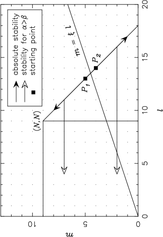
FIG. 1.: Stability lines of the recursions for the calculation of $I(l,m,-1)$. The solid arrows refer to the stable flux of the recursion (22). The open ones refer to the recursion (21), but only if $\alpha>\beta$. In the opposite case, the symmetric of Eq. (21) under $(l,\alpha)\leftrightarrow(m,\beta)$ exchange can be used to move downwards with stability.

REFERENCES

- [1] J. L. Calais, and P. O. Löwdin, J. Mol. Spect. 8, 203 (1962).
- [2] R. A. Sack, C. C. J. Roothaan, and W. Kolos, J. Math. Phys. 8, 1093 (1967).
- [3] A. J. Thakkar, and V.H. Smith, Jr., Phys. Rev. A15, 1 (1977).
- [4] G. Breit, Phys. Rev. 34, 553 (1929).
- [5] J. Caro, C. García Recio, and J. Nieves, preprint NUCL-TH 9801065, submitted to Nuc. Phys. A.
- [6] D. M. Fromm, and R. N. Hill, Phys. Rev. A36, 1013 (1987).
- [7] P. J. Roberts, J. Chem. Phys. 43 3547 (1965).
- [8] N. Solony, C. S. Lin, and F. W. Birss, J. Chem. Phys. 45, 976 (1966).
- [9] L. Hambro, Phys. Rev. A5, 2027 (1972).
- [10] G. F. Thomas, F. Javor, and S. M. Rothstein, J. Chem. Phys. 64, 1574 (1976).
- [11] F. W. King, Phys. Rev. A44, 7108 (1991).
- [12] Z-C. Yan, and G. W. F. Drake, Chem. Phys. Lett. 259, 96 (1996).
- [13] I. Porras, and F. W. King, Phys. Rev. A49, 1637 (1994).
- [14] Z-C. Yan, and G. W. F. Drake, J. Phys. B30, 4723 (1997).
- [15] C. L. Pekeris, Phys. Rev. 112, 1649 (1958).
- [16] M. Abramowitz, and I. A. Stegun, Handbook of Mathematical Functions (Dover Publications, New York, 1972).