Long-range interactions of metastable helium atoms

Abstract

Polarizabilities, dispersion coefficients, and long-range atom-surface interaction potentials are calculated for the $n=2$ triplet and singlet states of helium using highly accurate, variationally determined, wave functions.

The advent of doubled basis sets has made it possible to calculate precisely many properties of two-electron atomic systems [1, 2, 3, 4]. We apply variational methods developed previously and demonstrated for the helium atom [5] to calculate nonrelativistic values of the electric dipole, quadrupole, and octupole polarizabilities and corresponding dispersion coefficients for the metastable $n=2$ singlet and triplet states, respectively, He$(2\,^{1}\!S)$ and He$(2\,^{3}\!S)$. Additionally, potentials for the atom-wall interaction of a He$(2\,^{1}\!S)$ or a He$(2\,^{3}\!S)$ atom and a single perfectly conducting wall or a dielectric wall are calculated with the inclusion of retardation effects due to the finite speed of light. Our results for atom-wall interactions are germane to experiments involving atom-evanescent wave mirrors [6].

In this paper the notation of Ref. [7] is followed very closely; references to equations of Ref. [7] will be preceded by the symbol I. Atomic units are used throughout.

The dispersion interaction of two like atoms can be written

$$U(R)=-C_{6}R^{-6}-C_{8}R^{-8}-C_{10}R^{-10},$$ (1)

where the coefficients $C_{6}$, $C_{8}$, and $C_{10}$ are the van der Waals coefficients, $R$ is the interatomic distance, and

$$C_{6}=(3/\pi)G(1,1)\,,$$ (2)

$$C_{8}=(15/\pi)G(1,2)\,,$$ (3)

$$C_{10}=(28/\pi)G(1,3)+(35/\pi)G(2,2)\,,$$ (4)

with

$$G(l,m)=\int_{0}^{\infty}\alpha_{l}(i\omega)\alpha_{m}(i\omega)d\omega\,,$$ (5)

where $\alpha_{l}(i\omega)$ is the $2^{l}$-pole dynamic polarizability function evaluated at imaginary frequency defined by Eqs. (6)–(9) of Ref. [5], and similarly for $\alpha_{m}(i\omega)$.

When the effects of retardation due to the finite speed of light are considered the potential $U(R)$, Eq. (1), can be replaced by [8, 9]

$$V(R)=-C_{6}f_{6}(R)R^{-6}-C_{8}f_{8}(R)R^{-8}-C_{10}f_{10}(R)R^{-10},$$ (6)

The coefficient $f_{10}(R)$ will not be considered in this paper as the $C_{10}$ term is usually negligible. Expressions for the retardation coefficients, $f_{6}(R)$ and $f_{8}(R)$, as integrals involving the dynamic electric dipole polarizabilities, are given in Eqs. I-(5) and I-(7).

The form (6) intrinsically includes certain relativistic effects, so that when $f_{6}(R)$ and $f_{8}(R)$ are expanded in powers of the fine structure constant $\alpha_{\rm fs}=1/137.035\,989\,5$ for small distances

$$V(R)\sim-R^{-6}[C_{6}-\alpha_{\rm fs}^{2}R^{2}W_{4}]-R^{-8}[C_{8}-\alpha_{\rm fs}^{2}R^{2}W_{6}],$$ (7)

where

$$W_{4}=\frac{1}{\pi}\int_{0}^{\infty}d\omega\;\omega^{2}\alpha_{1}^{2}(i\omega)$$ (8)

and

$$W_{6}=\frac{3}{\pi}\int_{0}^{\infty}d\omega\;\omega^{2}\alpha_{1}(i\omega)\alpha_{2}(i\omega).$$ (9)

The relativistic origin of the coefficient $W_{4}$ has been discussed by Power and Zienau [10], see also [11]. The coefficient $W_{6}$ of the factor $\alpha_{\rm fs}^{2}/R^{6}$ in (7) corresponds to the theory of Power and Thirunamachandran [9] and is equal to the coefficient $W_{LL;4,2}$ in the theory of Meath and Hirschfelder based on the Breit-Pauli Hamiltonian [11]. As the distance increases retardation arising from the finite speed of light becomes important and the potential approaches its asymptotic form, see Eqs. I-(13) and I-(14),

$$V(R)\sim-K_{7}R^{-7}-K_{9}R^{-9},$$ (10)

with

$$K_{7}=\frac{23}{4\pi}\frac{\alpha_{1}^{2}(0)}{\alpha_{\rm fs}}=250.81\;\alpha_{1}^{2}(0),\qquad K_{9}=\frac{531}{16\pi}\frac{\alpha_{1}(0)\alpha_{2}(0)}{\alpha_{\rm fs}}=1\,447.6\;\alpha_{1}(0)\alpha_{2}(0).$$ (11)

An expression for the potential $V_{{\rm At}D}(R,\epsilon)$ for the interaction [12, 13] of an atom and a dielectric wall was presented in Eq. I-(15), where $R$ is the atom-wall distance and $\epsilon$ is the dielectric constant of the wall. The expression is a double integral that can be evaluated with knowledge of the function $\alpha_{1}(i\omega)$. For small distances $V_{{\rm At}D}(R,\epsilon)$ has the limiting form

$$V_{{\rm At}D}(R,\epsilon)\sim-\frac{C_{3}}{R^{3}}\frac{\epsilon-1}{\epsilon+1},$$ (12)

where

$$C_{3}=\frac{1}{4\pi}\int_{0}^{\infty}d\omega\alpha_{1}(i\omega).$$ (13)

As the separation increases retardation becomes important and the potential approaches its asymptotic form,

$$V_{{\rm At}D}(R,\epsilon)\sim-\frac{K_{4}}{R^{4}}\frac{\epsilon-1}{\epsilon+1}\phi(\epsilon),$$ (14)

where $\phi(\epsilon)$ is given in Eq. I-(21) and

$$K_{4}=3\alpha_{1}(0)/(8\pi\alpha_{\rm fs})=16.357\,\alpha_{1}(0).$$ (15)

For a perfectly conducting wall $V_{{\rm At}D}(R,\epsilon)$ reduces to $V_{{\rm At}M}(R)$, where

$$V_{{\rm At}M}(R)\equiv V_{{\rm At}D}(R,\infty)=-C_{3}f_{3}(R)R^{-3}$$ (16)

and the retardation coefficient $f_{3}(R)$ is an integral involving $\alpha_{1}(i\omega)$ and is given in Eq. I-(26). For small distances $V_{{\rm At}M}(R)\sim-C_{3}/R^{3}$ and for asymptotically large distances $V_{{\rm At}M}(R)\sim-K_{4}/R^{4}$. Table II of Ref. [14] summarizes the various limits of $V_{{\rm At}D}(R,\epsilon)$.

It has been shown that double basis sets work well for calculations involving $S$ states of helium [3]. The basis set used here was constructed as in Ref. [5] with basis set functions expressed using Hylleraas coordinates

$$\{\chi_{ijk}(\alpha,\beta) = r_{1}^{i}\,r_{2}^{j}\,r_{12}^{k}\,e^{-\alpha r_{1}-\beta r_{2}}\}\,.$$ (17)

The explicit form for the wave function is

$$\Psi({\rm\bf r}_{1},{\rm\bf r}_{2}) = \sum_{ijk}\,[a_{ijk}^{(1)}\,\chi_{ijk}(\alpha_{1},\beta_{1})+a_{ijk}^{(2)}\,\chi_{ijk}(\alpha_{2},\beta_{2})]\pm\,{\rm exchange}\,,$$ (18)

and $i+j+k\leq\Omega$. The convergence of the eigenvalues is studied as $\Omega$ is progressively enlarged. Finally, a complete optimization is performed with respect to the two sets of nonlinear parameters $\alpha_{1}$, $\beta_{1}$, and $\alpha_{2}$, $\beta_{2}$ by first calculating the derivatives analytically in

$${\partial E}\over{\partial\alpha} = 2\bigg{\langle}\Psi\bigg{|}H\bigg{|}{{\partial\Psi}\over{\partial\alpha}}\bigg{\rangle}-2E\bigg{\langle}\Psi\bigg{|}{{\partial\Psi}\over{\partial\alpha}}\bigg{\rangle}\,,$$ (19)

where $\alpha$ represents any nonlinear parameter, $E$ is the trial energy, $H$ is the Hamiltonian, and $\langle\Psi|\Psi\rangle=1$ is assumed, and then locating the zeros of the derivatives by Newton’s method. These techniques yield much improved convergence relative to single basis set calculations. The method of the evaluation of the two-electron integrals in Hylleraas coordinates can be found in Ref. [15].

The expressions for the dynamic dipole polarizabilities, Eqs. (6)–(9) of Ref. [5], were evaluated using the wave functions determined by the variational method. Values of the static polarizabilities are given in Table I for He($2\,^{1}\!S$) and He($2\,^{3}\!S$). The polarizabilities given in Table I are extrapolated results, with the convergence studied as in Refs. [3] and [5], and the estimated extrapolation error in the last digit is given in parentheses with the listed values. The largest basis set sizes used consisted of 616 functions for the $S$ states, 910 functions for the $P$ states, $931$ functions for the $D$ states, and 1092 functions for the $F$ states. The converged results are compared with some previous calculations and experiments in Table II and III. Ekstrom et al. [16] determined the He($2\,^{3}\!S$) polarizability by combining their measured Na polarizability with the Molof et al. [17] measurement of the Na polarizability relative to the polarizability of He($2\,^{3}\!S$). For the triplet state the experimental values of Ref. [18] and of Refs. [16, 17] and the bounds of Glover and Weinhold are compared with our calculated polarizability in Fig. 1.

The dynamic polarizability functions were constructed using the largest basis sets of each symmetry and used to evaluate the atom-atom dispersion constants and retardation coefficients. Our results for the dispersion constants are given in Table IV, with the estimated convergence errors given in parentheses, and the results are compared to other calculations in Tables V and VI. The retardation coefficients are given in Table VII and Fig. 2.

Chen and Chung [19] calculated the coefficients $W_{4}$ and $W_{6}$ for He($2\,^{1}\!S$) and their results are compared with ours in Table VIII; their published value of $W_{6}$ was multiplied by the factor $\frac{3}{2}$ to correspond to the theory of Ref. [9] and the agreement is very good.

For the atom-wall interactions the values of the coefficients $C_{3}$ can be obtained from the alternate expression

$$C_{3}=\frac{1}{12}\left\langle 0\left|\left(\sum_{i=1}^{N}{\bf r}_{i}\right)^{2}\right|0\right\rangle,$$ (20)

which follows from integration of Eq. (13), where $N$ is the number of electrons and $|0\rangle$ is accordingly the $2\,^{1}\!S$ or the $2\,^{3}\!S$ wave function. Since high-precision matrix elements are available [4, 20] Eq. (20) was used to obtain the coefficients $C_{3}(2\,^{1}\!S)=2.671\,212\,717\,025$ and $C_{3}(2\,^{3}\!S)=1.900\,924\,084\,097$.

The dynamic dipole polarizability was used to evaluate the potential for various dielectric walls. Results for He$(2\,^{1}\!S)$ are given in Table IX and Fig. 3 and those for He$(2\,^{3}\!S)$ are given in Table X and Fig. 4. The dielectric materials represented in the tables correspond to fused silica ($\epsilon=2.123$), BK-7 glass ($\epsilon=2.295$), and a GaAs-type material ($\epsilon=3.493$). The tabulated potentials may be helpful in planning and analyzing experiments with atom-evanescent wave mirrors, see for example Ref. [6].

We thank Professor G. W. F. Drake and Dr. P. L. Bouyer for helpful communications. The Institute for Theoretical Atomic and Molecular Physics is supported by a grant from the National Science Foundation to the Smithsonian Institution and Harvard University. ZCY was also supported by the Natural Sciences and Engineering Research Council of Canada.

TABLE I.: Values of the static polarizabilities $\alpha_{1}(0)$, $\alpha_{2}(0)$, and $\alpha_{3}(0)$ for the $2\,^{1}\!S$ and $2\,^{3}\!S$ states of He. Numbers in parentheses represent the estimated error in the last digit of the listed, extrapolated value.

State	$\alpha_{1}(0)$	$\alpha_{2}(0)$	$\alpha_{3}(0)$
$2{}^{1}S$	800.316 33(7)	7 106.053 7(5)	293 703.50(6)
$2{}^{3}S$	315.631 468(12)	2 707.877 3(3)	88 377.325 3(7)

TABLE II.: Comparison of static multipole polarizabilities $\alpha_{1}(0)$, $\alpha_{2}(0)$, and $\alpha_{3}(0)$ for He($2\,^{1}\!S$). For the experimental value numbers in parenthesis give the quoted error.

Author (year)	Ref.	$\alpha_{1}(0)$		$\alpha_{2}(0)$		$\alpha_{3}(0)$
Crosby and Zorn (77) Expt.	[18]	729	(88)
Chung and Hurst (66)	[21]	801	.9
Drake (72)	[22]	800	.2
Chung (77)	[23]	801	.10
Glover and Weinhold (77)	[24]	803	.31$\pm$6.61a
Lamm and Szabo (80), ECA	[25]	790	.8
Rérat et al. (93)	[26]	803	.25	6870	.9
Chen (95)	[27]	800	.34
This work		800	.316 33(7)	7 106	.053 7(5)	293 703	.50(6)

TABLE III.: Comparison of static multipole polarizabilities $\alpha_{1}(0)$, $\alpha_{2}(0)$, and $\alpha_{3}(0)$ for He($2\,^{3}\!S$).

Author (year)	Ref.	$\alpha_{1}(0)$		$\alpha_{2}(0)$		$\alpha_{3}(0)$
Crosby and Zorn (77) Expt.	[18]	301	(20)
Ekstrom et al. (95) Expt.	[16, 17]	322	(6.8)
Bishop and Pipin (93)	[28]	315	.631	2 707	.85	88 377	.2
Rérat et al. (93)	[26]	315	.92	2 662	.02
Glover and Weinhold (77)	[24]	316	.24$\pm$0.78b
Drake (72)	[22]	315	.608
Chung (77)	[23]	315	.63
Chen and Chung (96), $B$ Spline	[19]	315	.63	2 707	.89	88 377	.4
Chen and Chung (96), Slater	[19]	315	.611	2 707	.81	88 356	.2
Chung and Hurst (66)	[21]	315	.63
Chen (95)	[27]	315	.633
This work		315	.631 468(12)	2 707	.877 3(3)	88 377	.325 3(7)

TABLE IV.: Values of $C_{6}$, $C_{8}$, and $C_{10}$ for the interaction of two He atoms.

System	$C_{6}$	$C_{8}$	$C_{10}$
$2\,^{1}\!S$-$2\,^{1}\!S$	11 241.052(5)	817 250.5(4)	108 167 630(54)
$2\,^{3}\!S$-$2\,^{3}\!S$	3 276.680 0(3)	210 566.55(6)	21 786 760(5)

TABLE V.: Comparison of $C_{6}$, $C_{8}$, and $C_{10}$ for the He($2\,^{1}\!S$)-He($2\,^{1}\!S$) system.

Author (year)	Ref.	$C_{6}$		$C_{8}$		$C_{10}$
Glover and Weinhold (77)	[29]	11 330	$\pm$630c
Rérat et al. (93)	[26]	11 360		812 500
Victor et al. (68)	[30]	11 300
Lamm and Szabo (80), ECA	[25]	10 980
Chen (95)	[31]	11 244		817 360		108 184 000
This work		11 241	.052(5)	817 250	.5(4)	108 167 630	(54)

TABLE VI.: Comparison of $C_{6}$, $C_{8}$, and $C_{10}$ for the He($2\,^{3}\!S$)-He($2\,^{3}\!S$) system.

Author (year)	Ref.	$C_{6}$		$C_{8}$		$C_{10}$
Glover and Weinhold (77)	[29]	3 289	$\pm$90d
Victor et al. (68)	[30]	3 290
Lamm and Szabo (80), ECA	[25]	3 300
Rérat et al. (93)	[26]	3 279		208 600
Bishop and Pipin (93)	[28]	3 276	.677 0	210 563	.99	21 786 484
Chen (95)	[31]	3 276	.1	210 520		21 783 800
Chen and Chung (96), $B$ spline	[19]	3 276	.10	210 518		21 783 800
Chen and Chung (96), Slater	[19]	3 275	.90	210 507		21 780 200
This work		3 276	.680 0(3)	210 566	.55(6)	21 786 760	(5)

TABLE VII.: The dimensionless retardation coefficients $f_{6}(R)$ and $f_{8}(R)$ for the atom-atom interaction. The dispersion coefficients $C_{6}$ and $C_{8}$ are also given. In the last line, labeled “Asymptotic” the values calculated using the asymptotic forms $f_{6}\sim K_{7}/(RC_{6})$ and $f_{8}\sim K_{9}/(RC_{8})$ are given in, respectively cols. 2,4 and cols. 3,5, with $K_{7}$ and $K_{9}$ given in Eq. (11).

	He($2\,^{1}\!S$)-He($2\,^{1}\!S$)		He($2\,^{3}\!S$)-He($2\,^{3}\!S$)
	$C_{6}$	$C_{8}$	$C_{6}$	$C_{8}$
	112 41.052(5)	817 250.5(4)	3 276.680 0(3)	210 566.55(6)
$R$	$f_{6}(R)$	$f_{8}(R)$	$f_{6}(R)$	$f_{8}(R)$
10	0.999998	0.999996	0.999995	0.999992
15	0.999996	0.999992	0.999988	0.999982
20	0.999993	0.999986	0.999980	0.999969
25	0.999989	0.999978	0.999968	0.999952
30	0.999984	0.999968	0.999955	0.999931
50	0.999958	0.999913	0.999879	0.999812
70	0.999919	0.999833	0.999770	0.999638
100	0.999840	0.999666	0.999548	0.999281
150	0.999655	0.999271	0.999034	0.998446
200	0.999408	0.998742	0.998358	0.997337
250	0.999106	0.998088	0.997533	0.995980
300	0.998750	0.997318	0.996573	0.994397
500	0.996857	0.993223	0.991568	0.986162
700	0.994325	0.987790	0.985052	0.975560
1000	0.989563	0.977772	0.973189	0.956657
1500	0.979675	0.957749	0.949690	0.920633
2000	0.968032	0.935332	0.923467	0.882350
2500	0.955170	0.911784	0.895919	0.843974
3000	0.941459	0.887865	0.867915	0.806627
5000	0.882570	0.795572	0.759993	0.675026
7000	0.822962	0.714364	0.666219	0.572701
10000	0.739435	0.614288	0.554000	0.460880
15000	0.622323	0.492124	0.424424	0.342480
20000	0.530963	0.407029	0.340027	0.270048
25000	0.459732	0.345261	0.282000	0.221929
30000	0.403520	0.298792	0.240136	0.187921
50000	0.266133	0.191769	0.149197	0.115667
70000	0.196376	0.140118	0.107696	0.083251
100000	0.140107	0.099381	0.075824	0.058519
	Asymptotic
100000	0.142912	0.100738	0.076257	0.058760

TABLE VIII.: The coefficients $W_{4}$ and $W_{6}$ appearing in the expansion of the atom-atom interaction potential at small distances, see Eq. (7).

	Ref.	$W_{4}$		$W_{6}$
He($2\,^{1}\!S$)-He($2\,^{1}\!S$)	This work	3	.912 7(5)	555	.86(5)
He($2\,^{3}\!S$)-He($2\,^{3}\!S$)	Chen and Chung [19]	3	.3006	314	.18e
	This work	3	.305 2(5)	314	.44(5)

TABLE IX.: For He($2\,^{1}\!S$), values of $-R^{3}V_{{\rm At}D}(R,\epsilon)$, where $V_{{\rm At}D}(R,\epsilon)$ is the atom-wall potential, for values of $\epsilon$ corresponding to several types of dielectric, cols. 2–4, and in col. 5 values of $-R^{3}V_{{\rm At}M}(R)$ for a perfectly conducting wall. The coefficient $C_{3}(2\,^{1}\!S)$ is 2.67121.

$R$	$\epsilon=2.123$	$\epsilon=2.295$	$\epsilon=3.493$	$\epsilon=\infty$
10	0.95339	1.04221	1.47123	2.65990
15	0.95029	1.03882	1.46644	2.65455
20	0.94739	1.03564	1.46194	2.64938
25	0.94463	1.03262	1.45768	2.64439
30	0.94200	1.02975	1.45361	2.63956
50	0.93244	1.01928	1.43883	2.62159
70	0.92395	1.00999	1.42570	2.60532
100	0.91253	0.99750	1.40805	2.58320
150	0.89577	0.97916	1.38214	2.55042
200	0.88087	0.96286	1.35913	2.52098
250	0.86726	0.94797	1.33812	2.49381
300	0.85463	0.93415	1.31863	2.46833
500	0.81082	0.88624	1.25109	2.37768
700	0.77415	0.84615	1.19462	2.29898
1000	0.72765	0.79532	1.12305	2.19547
1500	0.66478	0.72660	1.02637	2.04896
2000	0.61386	0.67095	0.94810	1.92470
2500	0.57109	0.62421	0.88236	1.81635
3000	0.53433	0.58405	0.82587	1.72023
5000	0.42573	0.46540	0.65887	1.41942
7000	0.35344	0.38641	0.54755	1.20473
10000	0.28060	0.30682	0.43519	0.97660
15000	0.20730	0.22670	0.32187	0.73525
20000	0.16342	0.17873	0.25390	0.58540
25000	0.13443	0.14702	0.20893	0.48434
30000	0.11395	0.12463	0.17715	0.41205
50000	0.07032	0.07692	0.10938	0.25591
70000	0.05067	0.05543	0.07883	0.18478
100000	0.03565	0.03899	0.05545	0.13013

TABLE X.: For He($2\,^{3}\!S$), values of $-R^{3}V_{{\rm At}D}(R,\epsilon)$, where $V_{{\rm At}D}(R,\epsilon)$ is the atom-wall potential, for values of $\epsilon$ corresponding to several types of dielectric, cols. 2–4, and in col. 5 values of $-R^{3}V_{{\rm At}M}(R)$ for a perfectly conducting wall. The coefficient $C_{3}(2\,^{3}\!S)$ is 1.90092.

$R$	$\epsilon=2.123$	$\epsilon=2.295$	$\epsilon=3.493$	$\epsilon=\infty$
10	0.67644	0.73946	1.04384	1.88963
15	0.67336	0.73608	1.03907	1.88428
20	0.67047	0.73292	1.03459	1.87912
25	0.66773	0.72992	1.03036	1.87413
30	0.66512	0.72707	1.02633	1.86931
50	0.65566	0.71671	1.01169	1.85142
70	0.64728	0.70755	0.99875	1.83525
100	0.63606	0.69527	0.98140	1.81333
150	0.61966	0.67733	0.95607	1.78095
200	0.60516	0.66146	0.93368	1.75197
250	0.59196	0.64703	0.91333	1.72529
300	0.57977	0.63370	0.89454	1.70030
500	0.53788	0.58789	0.83004	1.61162
700	0.50336	0.55016	0.77695	1.53484
1000	0.46046	0.50328	0.71103	1.43436
1500	0.40433	0.44195	0.62481	1.29413
2000	0.36074	0.39433	0.55783	1.17825
2500	0.32560	0.35593	0.50380	1.08034
3000	0.29654	0.32419	0.45909	0.99640
5000	0.21739	0.23769	0.33709	0.75412
7000	0.17046	0.18640	0.26458	0.60138
10000	0.12784	0.13981	0.19860	0.45715
15000	0.08946	0.09785	0.13907	0.32318
20000	0.06848	0.07490	0.10649	0.24852
25000	0.05536	0.06055	0.08610	0.20136
30000	0.04641	0.05076	0.07219	0.16904
50000	0.02810	0.03074	0.04372	0.10257
70000	0.02012	0.02201	0.03131	0.07350
100000	0.01411	0.01543	0.02195	0.05154

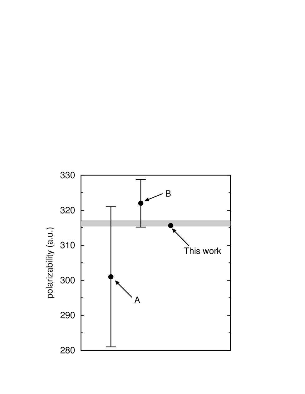
FIG. 1.: Comparison of measured values (A, B) and the upper and lower bounds of Glover and Weinhold (shaded region) [29] with the present calculation of the static polarizability for He($2\,^{3}\!S$). The point A is the measurement of Crosby and Zorn [18] and the point B is that of Ekstrom et al. [16] determined in combination with measurements from Molof et al. [17].

FIG. 2.: Dimensionless retardation coefficients for He($2\,^{1}\!S$) (solid line) and He($2\,^{3}\!S$) (dashed line).

FIG. 3.: Potentials $R^{3}V(R)$ for He($2\,^{1}\!S$) atom-wall interactions. The labels A, B, and C correspond, respectively, to dielectric constants $\epsilon$ of 2.123, 2.295, and 3.493.

FIG. 4.: Potentials $R^{3}V(R)$ for He($2\,^{3}\!S$) atom-wall interactions. The labels A, B, and C correspond respectively, to dielectric constants $\epsilon$ of 2.123, 2.295, and 3.493.

REFERENCES

- [1] G. W. F. Drake, in Long Range Forces: Theory and Recent Experiments in Atomic Systems, edited by F. S. Levin and D. Micha (Plenum Press, New York, 1992).
- [2] G. W. F. Drake and Z.-C. Yan, Phys. Rev. A 46, 2378 (1992).
- [3] G. W. F. Drake and Z.-C. Yan, Chem. Phys. Lett. 229, 486 (1994).
- [4] G. W. F. Drake, in Atomic, molecular, and optical physics handbook, edited by G. W. F. Drake (American Institute of Physics, Woodbury, NY, 1996), p. 154.
- [5] Z.-C. Yan, J. F. Babb, A. Dalgarno, and G. W. F. Drake, Phys. Rev. A 54, 2824 (1996).
- [6] A. Landragin et al., Phys. Rev. Lett. 77, 1464 (1996).
- [7] Z.-C. Yan, A. Dalgarno, and J. F. Babb, Phys. Rev. A 55, 2882 (1997).
- [8] H. B. G. Casimir and D. Polder, Phys. Rev. 73, 360 (1948).
- [9] E. A. Power and T. Thirunamachandran, Phys. Rev. A 53, 1567 (1996).
- [10] E. A. Power and S. Zienau, J. Franklin Inst. 263, 403 (1957).
- [11] W. J. Meath and J. O. Hirschfelder, J. Chem. Phys. 44, 3210 (1966).
- [12] I. E. Dzyaloshinskii, E. M. Lifshitz, and L. P. Pitaevskii, Adv. Phys. 10, 165 (1961).
- [13] Y. Tikochinsky and L. Spruch, Phys. Rev. A 48, 4223 (1993).
- [14] F. Zhou and L. Spruch, Phys. Rev. A 52, 297 (1995).
- [15] Z.-C. Yan and G. W. F. Drake, Chem. Phys. Lett. 259, 96 (1996).
- [16] C. R. Ekstrom et al., Phys. Rev. A 51, 3883 (1995).
- [17] R. W. Molof, H. L. Schwartz, T. M. Miller, and B. Bederson, Phys. Rev. A 10, 1131 (1974).
- [18] D. A. Crosby and J. C. Zorn, Phys. Rev. A 16, 488 (1977).
- [19] M.-K. Chen and K. T. Chung, Phys. Rev. A 53, 1439 (1996).
- [20] G. W. F. Drake, private communication, 1997.
- [21] K. T. Chung and R. P. Hurst, Phys. Rev. 152, 35 (1966).
- [22] G. W. F. Drake, Can. J. Phys. 50, 1896 (1972).
- [23] K. T. Chung, Phys. Rev. A 15, 1347 (1977).
- [24] R. M. Glover and F. Weinhold, J. Chem. Phys. 66, 185 (1977).
- [25] G. Lamm and A. Szabo, J. Chem. Phys. 72, 3354 (1980).
- [26] M. Rérat, M. Caffarel, and C. Pouchan, Phys. Rev. A 48, 161 (1993).
- [27] M.-K. Chen, J. Phys. B 28, 1349 (1995).
- [28] D. M. Bishop and J. Pipin, Int. J. Quant. Chem. 47, 129 (1993).
- [29] R. M. Glover and F. Weinhold, J. Chem. Phys. 66, 191 (1977).
- [30] G. A. Victor, A. Dalgarno, and A. J. Taylor, J. Phys. B 1, 13 (1968).
- [31] M.-K. Chen, J. Phys. B 28, 4189 (1995).