Transverse quasilinear relaxation in inhomogeneous magnetic field

Abstract

Transverse quasilinear relaxation of the cyclotron-Cherenkov instability in the inhomogeneous magnetic field of pulsar magnetospheres is considered. We find quasilinear states in which the kinetic cyclotron-Cherenkov instability of a beam propagating through strongly magnetized pair plasma is saturated by the force arising in the inhomogeneous field due to the conservation of the adiabatic invariant. The resulting wave intensities generally have nonpower law frequency dependence, but in a broad frequency range can be well approximated by the power law with the spectral index $-2$. The emergent spectra and fluxes are consistent with the one observed from pulsars.

I Introduction

In this paper we consider quasilinear relaxation in inhomogeneous magnetic field of a highly relativistic beam propagating along the strong magnetic field through a pair plasma. This describes the physical conditions on the open field lines of pulsar magnetospheres (e.g. [1]). The possibility of the cyclotron-Cherenkov instability of the beam in the pulsar magnetosphere has been suggested by [2] and [3] and developed later by [4], [5], [6]. The cyclotron-Cherenkov instability develops at the anomalous Doppler resonance

$$\,\omega({\bf k})-k_{\parallel}v_{\parallel}-s{\,\omega_{B}\over\gamma}=0\,\,\mbox{ for $s<0$}$$ (1)

where $\,\omega({\bf k})$ is the frequency of the normal mode, ${\bf k}$ is a wave vector, $v$ is the velocity of the resonant particle, $\,\omega_{B}=|q|B/mc$ is the nonrelativistic gyrofrequency, $\,\gamma$ is the Lorentz factor in the pulsar frame, $q$ is the charge of the resonant particle, $m$ is its mass and $c$ is the speed of light. It has been shown (e.g. [6]), that cyclotron-Cherenkov instability can explain a broad variety of the observed pulsar phenomena.

Close to the stellar surface, where the initial beam is produced and accelerated, the particles quickly reach their ground gyrational state due to the sychrotron emission in a superstrong magnetic field, so that their distribution becomes virtually one dimensional [1]. In the outer parts of magnetosphere it becomes possible to satisfy the anomalous Doppler resonance - the cyclotron-Cherenkov instability develops bringing about the diffusion of particles in transverse moments. The relevant saturation mechanism then determines the final spectrum (which can be later modified be the absorption processes).

The nonlinear saturation of the cyclotron-Cherenkov instability due to the diffusion of the resonant particles has been previously considered by several authors. Kawamura & Suzuki [2] neglected the possible stabilizing effects of the radiation reaction force due to the cyclotron emission at the normal Doppler resonance and the force arizing in the inhomogeneous magnetic field due to the conservation of the adiabatic invariant. These forces result in a saturation of the quasilinear diffusion.

Lominadze et al. [3] were the first to notice the importance of the radiation reaction force due to the emission at the normal Doppler resonance on the saturation of the quasilinear diffusion. Unfortunately, Lominadze et al. [3] used an expression for the cyclotron damping rates which is applicable only for the nonrelativistic transverse motions, when $\gamma\psi$ ($psi$ is the pitch angle) is much less than unity. In the pulsar magnetospheres the development of the cyclotron-Cherenkov instability results in a diffusion of particles in transverse moments, quickly increasing there transverse energy to relativistic values.

In a review paper Lominadze et al. [7] took a correct account of the radiation reaction force due to the emission at the normal Doppler resonance and pointed out the importance of the the force arizing in the inhomogeneous magnetic field due to the conservation of the adiabatic invariant ( ${\bf G}$ force Eq. (17)). When considering the deceleration of the beam Lominadze et al. [7] has incorrectly neglected the radiation reaction force due to the emission at the anomalous Doppler resonance in comparison with the radiation reaction force due to the emission at the normal Doppler resonance.

In this work we reconsider and extend the treatment of the quasilinear stage of the cyclotron-Cherenkov instability. We have found a state, in which the particles are constantly slowing down their parallel motion, mainly due to the component along magnetic field of the radiation reaction force of emission at the anomalous Doppler resonance. At the same time they keep the pitch angle almost constant due to the balance of the force ${\bf G}$ and the component perpendicular to the magnetic field of the radiation reaction force of emission at the anomalous Doppler resonance. We calculate the distribution function and the wave intensities for such quasilinear state.

In the process of the quasilinear diffusion the initial beam looses a large fraction of its initial energy $\approx 10\%$, which is enough to explain the typical luminosities of pulsars. Though the quasisteady wave intensities are not strictly power laws (see Eq. (46)), they can well approximated by a power law with a spectral index $F(\nu)\propto-2$ ($F(\nu)$ is the spectral flux density in Janskys) which is very close to the observed mean spectral index of $-1.6$ [8]. The predicted spectra also show a turn off at the low frequencies $\nu\leq 300MHz$ and a flattering of spectrum at large frequencies $\nu\geq 1GHz$ which may be related to the possible turn-up in the flux densities at mm-wavelengths [9].

II Quasilinear Diffusion

A particle moving in a dielectric medium in magnetic field with the velocity larger than the velocity of light in a medium is emitting electromagnetic waves at the anomalous Doppler resonance ( $s<0$ in Eq. (1)) and at the normal Doppler resonance ( $s>0$ in Eq. (1)). The radiation reaction due to the emission at the normal Doppler resonance slows the particle’s motion along magnetic field and decreases its transverse momentum. The radiation reaction due to the emission at the anomalous Doppler resonance increases its transverse momentum and also slows the particle’s motion along magnetic field [10]. As the particle propagates into the region of lower magnetic field, the force ${\bf G}$ decreases the its transverse momentum and increases the parallel momentum. The stationary state in transverse moments may be reach when the actions of the ${\bf G}$ force and radiation reaction due to the emission at the normal Doppler resonance is balanced by the radiation reaction due to the emission at the anomalous Doppler resonance.

The quasisteady stage may also be considered in terms of a detailed balance of for the particle transitions between the Landau levels. The quasisteady stage is reached when the number of induced transitions $up$ in Landau levels due to the emission at the anomalous Doppler resonance is balanced by the number of the spontaneous transitions $down$ in Landau levels due to the emission at the anomalous Doppler resonance.

The equations describing the quasilinear diffusion in the magnetic field are

$${df({\bf p})\over dt}={1\over\sin\psi}{\partial\over\partial\psi}\left[\sin\psi\left(D_{\psi\psi}\,{\partial\over\partial\psi}+D_{\psi p}{\partial\over\partial p}\right)f({\bf p})\right]\mbox{}$$ (2)

$$\hskip 21.68121pt{1\over p^{2}}{\partial\over\partial p}\left[p^{2}\left(D_{p\psi}{\partial\over\partial\psi}+D_{pp}{\partial\over\partial p}\right)f({\bf p})\right]\mbox{}$$ (3)

$$\left(\begin{array}[]{cc}D_{\psi\psi}\\ D_{\psi p}=D_{p\psi}\\ D_{pp}\end{array}\right)=\,\sum_{s<0}\int{d{\bf k}\over(2\pi)^{3}}w(s,{\bf p},{\bf k})n({\bf k})\left(\begin{array}[]{cc}(\Delta\psi)^{2}\\ (\Delta\psi)(\Delta p)\\ (\Delta p)^{2}\end{array}\right)\mbox{}$$ (10)

$${dn({\bf k})\over dt}=\sum_{s<0}\int d{\bf p}w(s,{\bf p},{\bf k})\left(n({\bf k})\hbar\left({\partial\over\partial p}+{\cos\psi-(kv/\omega)\cos\theta\over p\sin\psi}{\partial\over\partial\psi}\right)f({\bf p})\right)$$ (11)

Where

$$\Delta p={\hbar\omega\over v}\hskip 14.45377pt\Delta\psi={\hbar(\omega\cos\psi-k_{\parallel}v)\over pv\sin\psi}\mbox{}$$ (12)

$$n({\bf k})={E^{2}({\bf k})\over\hbar\omega({\bf k})}\mbox{}$$ (13)

$$w(s,{\bf p},{\bf k})={8\pi^{2}q^{2}R_{E}({\bf k})\over\hbar\omega({\bf k})}\left|{\bf e}({\bf k})\cdot{\bf V}(s,{\bf p},{\bf k})\right|^{2}\delta(\omega({\bf k})-s\omega_{B}/\gamma-k_{\parallel}v_{\parallel})\mbox{}$$ (14)

$${\bf V}(s,{\bf p},{\bf k})=\left(v_{\perp}{s\over z}J_{s}(z),\,-i\sigma sv_{\perp}J_{s}(z)^{\prime},v_{\parallel}J_{s}(z)\right)$$ (15)

where $E^{2}({\bf k})d{\bf k}/(2\pi)^{3}$ is the energy density of the waves in the unit element range of ${\bf k}$-space. In the Table I we give the dimensions of the main used quantities.

In Eq. (3) we neglected the spontaneous emission processes at the anomalous Doppler resonance and the induced emission processes at the normal Doppler resonance. The net effect of the spontaneous emission at the normal Doppler resonance is treated as a damping force acting on each particle in the Boltzman-type left hand side of equation (16). To be exact, we should have treated the effects of spontaneous emission at the normal Doppler resonance as stochastic terms in the Fokker-Plank-type terms on the right hand side of equation (16). But the fact that the emission at the normal Doppler resonance occurs on very high frequencies at which the presence of a medium is unimportant in the dispersion relation of the waves and can be neglected allows one to integrate the corresponding terms over angles and sum over harmonics to obtain a classical synchrotron radiation damping force, that can be treated using the Boltzman approach. Thus, the total time derivative of the distribution function is

$${df({\bf p})\over dt}={\partial f({\bf p})\over\partial t}+{\bf v}{\partial f({\bf p})\over\partial{\bf r}}+{\partial\over\partial{\bf p}}\left[\left({\bf G+F}+{q\over c}\left({\bf v}\times{\bf B_{0}}\right)\right)f({\bf p})\right]$$ (16)

where ${\bf G}$ is the force due to the conservation of the adiabatic invariant

$$G_{\parallel}=-\beta\gamma\psi^{2},\hskip 14.45377ptG_{\perp}=-\beta\gamma\psi,\hskip 14.45377pt\beta={mc^{2}\over R_{B}}$$ (17)

Here $R_{B}\approx 10^{9}$ cm is the radius of curvature and ${\bf F}$ is the radiation damping force due to the spontaneous synchrotron emission at the normal Doppler resonance:

$$F_{\parallel}=-\alpha\gamma^{2}\psi^{2},\hskip 14.45377ptF_{\perp}=-\alpha\psi\left(1+\gamma^{2}\psi^{2}\right),\hskip 14.45377pt\alpha={2q^{2}\omega_{B}^{2}\over 3c^{2}}$$ (18)

From (17) and (19) we find that

$${F_{\parallel}\over G_{\parallel}}={\alpha\over\beta}\gamma,\hskip 14.45377pt{F_{\perp}\over G_{\perp}}={\alpha\over\beta}\gamma\psi^{2},\,\,\mbox{ for $\gamma\psi\gg 1$}$$ (19)

where $r_{L}=c/\omega_{B}$ is a Larmor radius and $r_{e}=q^{2}/(mc^{2})=2.8\times 10^{-13}$cm is a classical radius of an electron.

The dimensionless ration in (19) is

$${\alpha\over\beta}={2R_{B}r_{e}\over r_{L}^{2}}=5\times 10^{-4}\,R_{B,9}R_{9}^{-6}$$ (20)

$R_{B,9}=R_{B}/10^{9}{\rm cm}$ is the radius of curvature in units of $10^{9}$ cm, $R_{9}=R/10^{9}{\rm cm}$ is the distance from the neutron star surface in units of $10^{9}$ cm.

Using (20) we find that for the primary particles with $\gamma\approx 10^{7}$

$${F_{\parallel}\over G_{\parallel}}\gg 1\mbox{}$$ (21)

$${F_{\perp}\over G_{\perp}}\ll 1,\hskip 14.45377pt\mbox{ for $\psi\ll\sqrt{{r_{L}^{2}\over 2R_{B}r_{e}\gamma}}\approx 10^{-2}$ }$$ (22)

Then the total derivative (16) may be written as

$${df({\bf p})\over dt}={\partial f({\bf p})\over\partial t}+{\bf v}{\partial f({\bf p})\over\partial{\bf r}}+{1\over p\sin\psi}{\partial\over\partial\psi}\left(\sin\psi G_{\perp}f({\bf p})\right)+{1\over p^{2}}{\partial\over\partial p}\left(p^{2}F_{\parallel}f({\bf p})\right)$$ (23)

We are interested in the quasilinear diffusion of the particles due to the resonant interaction with the waves at the anomalous Doppler effect. We expand the transition currents (15) in small $v_{\perp}$ keeping only $s=-1$ terms: ${\bf V}(-1,{\bf p},{\bf k})=v_{\perp}/2\left(1,i\sigma,0\right)$. Then for the waves propagating along magnetic field ${\bf e}({\bf k})=(1,0,0)$ we find

$$w(\pm 1,{\bf p},{\bf k})={\pi^{2}q^{2}v_{\perp}^{2}\over\hbar\omega({\bf k})}\delta(\omega({\bf k})-s\omega_{B}/\gamma-k_{\parallel}v_{\parallel})$$ (24)

where we took into account that $R_{E}({\bf k})\approx 1/2$.

We now can find the diffusion coefficients in the approximation of a one dimensional spectrum of the waves.

$$n({\bf k})={2\pi\delta(\theta)\over k^{2}\sin\theta}n(k),\hskip 14.45377ptn(k)=\int d{\bf\Omega_{k}}{k^{2}\over(2\pi)^{2}n({\bf k})}$$ (25)

We first note that we can simplify the change in the pitch angle (12) in the limit $\psi^{2}\ll\delta$ and $1/\gamma^{2}\ll\delta$

$$\Delta\psi\approx-{\hbar\omega\delta\over pv\sin\psi}$$ (26)

We then find

$$\left(\begin{array}[]{cc}D_{\psi\psi}\\ D_{\psi p}=D_{p\psi}\\ D_{pp}\end{array}\right)=\,\left(\begin{array}[]{cc}\phantom{{{{{a\over b}\over{a\over b}}}\over{{{a\over b}\over{a\over b}}}}}D\mbox{{${\delta\over\gamma^{2}}$}}E_{k}^{2}\left.\right|_{k=k_{res}}\\ \phantom{{{{{a\over b}\over{a\over b}}}\over{{{a\over b}\over{a\over b}}}}}-D\mbox{{${\psi mc\over\gamma}$}}E_{k}^{2}\left.\right|_{k=k_{res}}\\ \phantom{{{{{a\over b}\over{a\over b}}}\over{{{a\over b}\over{a\over b}}}}}D\mbox{{${\psi^{2}m^{2}c^{2}\over\delta}$}}E_{k}^{2}\left.\right|_{k=k_{res}}\end{array}\right),\hskip 14.45377ptD={\pi^{2}q^{2}\over m^{2}c^{3}}={\pi^{2}r_{e}\over mc}\hskip 7.22743pt$$ (27)

where

$$E_{k}^{2}=\hbar\omega(k)n(k)=\int{k^{2}d{\bf\Omega}\over(2\pi)^{2}}\hbar\omega({\bf k})n({\bf k})$$ (28)

is energy density per unit of one-dimensional wave vector and we assumed that $\omega({\bf k})$ is an isotropic function of ${\bf k}$.

We next solve the partial differential equation describing the evolution of the distribution function by sucsessive approximations. We first expand equation (3) in small $\psi$ assuming that $\partial/\partial\psi\simeq 1/\psi$. We also neglect the convection term assuming that the characteristic time for the development of the quasilinear diffusion is much smaller that the dynamic time of the plasma flow. Then we assume that it is possible to separate the distribution function into the parts depending on the $\psi$ and $p$:

$$f({\bf p})=Y(\psi,p)f(p)$$ (29)

with

$$f(p)=2\pi\int\sin\psi d\psi f({\bf p}),\hskip 14.45377pt\int dpp^{2}f(p)=1$$ (30)

In the lowest order in $\psi$ we obtain an equation:

$$-{1\over p\sin\psi}{\partial\over\partial\psi}\left(\sin\psi G_{\perp}Y(\psi)\right)={1\over\sin\psi}{\partial\over\partial\psi}\left[\sin\psi D_{\psi\psi}\,{\partial Y(\psi)\over\partial\psi}\right]$$ (31)

which has a solution

$$Y(\psi)={1\over\pi\psi_{0}^{2}}\exp\left(-{\psi^{2}\over\psi_{0}^{2}}\right),\hskip 14.45377pt\psi_{0}^{2}={Dmc\delta E_{k}^{2}\over\beta\gamma^{2}}={DR_{B}\delta E_{k}^{2}\over c\gamma^{2}}={\pi^{2}\delta R_{B}r_{e}E_{k}^{2}\over\gamma^{2}mc^{2}}$$ (32)

The next order in $\psi$ gives

$${\partial f({\bf p})\over\partial t}+{\partial\over\partial p}\left(F_{\parallel}f({\bf p})\right)={1\over\sin\psi}{\partial\over\partial\psi}\left[\sin\psi D_{\psi p}{\partial f({\bf p})\over\partial p}\right]+{1\over p^{2}}{\partial\over\partial p}\left[p^{2}D_{p\psi}{\partial f({\bf p})\over\partial\psi}\right]$$ (33)

By integrating (33) over $\psi$ with a weight $\psi$ we find the equation for the parallel distribution function:

$${\partial f(p)\over\partial t}-{\partial\over\partial p}\left({A}E_{k}^{2}\gamma^{2}f(p)\right)={2\over p^{2}}{\partial\over\partial p}\left(p{D}m^{2}c^{2}E_{k}^{2}f(p)\right)$$ (34)

where

$${A}={\alpha\psi_{0}^{2}\over E_{k}^{2}}={2q^{2}\omega_{B}^{2}\psi_{0}^{2}\over 3c^{2}E_{k}^{2}}={2\pi^{2}\omega_{B}^{2}q^{4}R_{B}\delta\over 3\gamma^{2}m^{2}c^{6}}={2\pi^{2}R_{B}r_{e}^{2}\delta\over 3\gamma^{2}r_{L}^{2}}$$ (35)

The term containing ${A}$ describes the slowing of the particles due to the radiation reaction force and the term containing $D$ describes the slowing of the particles due to the quasilinear diffusion, or, equivalently, due to the radiation reaction force of the anomalous Doppler resonance. To estimate the relative importance of these terms we consider a ratio

$${{A}\gamma^{3}\over{D}mc}={\alpha\delta\gamma\over\beta}={2\delta\gamma\over 3}{R_{B}r_{e}\over r_{L}^{2}}\ll 1$$ (36)

Neglecting the second term on the left hand side of (36) we find

$${\partial f(p)\over\partial t}-{2\over p^{2}}{\partial\over\partial p}\left(p{D}m^{2}c^{2}E_{k}^{2}f(p)\right)==0$$ (37)

If the cyclotron quasilinear diffusion has time to fully develop and reach a steady state, then the distribution function of the resonant particles is

$$f(p)\propto{1\over p\,E_{k}^{2}}$$ (38)

Next we turn to the equation describing the temporal evolution of the wave intensity (11). Neglecting the spontaneous emission term and the wave convection we find

$${\partial E_{k}^{2}\over\partial t}=-\Gamma E_{k}^{2}f(\gamma)_{res}$$ (39)

where

$$\Gamma={1\over f(\gamma)_{res}}\,\sum_{s}\int d{\bf p}w(s,{\bf p},{\bf k})\left(\hbar\left({\partial\over\partial p}+{\cos\psi-(kv/\omega)\cos\theta\over p\sin\psi}{\partial\over\partial\psi}\right)f({\bf p})\right)$$ (40)

and we introduced

$$f(\gamma)\gamma^{2}d\gamma=f(p)p^{2}dp$$ (41)

We will estimate this growth rate for the emission along the external magnetic field for distribution (30), (32). Neglecting $\partial/\partial p$ and assuming that $\psi^{2}\ll 2\delta$ (so that most of the particles are moving with the superluminal velocity) we find for $s=-1$

$$\Gamma={\pi\omega_{p,res}^{2}\over 2\omega}\gamma^{2}_{res}$$ (42)

(It is important to note that in the limit $\psi^{2}\ll 2\delta$ the growth rate does not depend on the scatter in pitch angles).

Equations (37) and (42) may be combined to a quasilinear expression

$${\partial\over\partial t}\left(f(\gamma)+{2\over p^{2}}{\partial\over\partial p}\left({p{D}m^{2}c^{2}E_{k}^{2}\over\Gamma}\right)\right)=0$$ (43)

Which after integration gives

$$f(\gamma)-{2\over\gamma^{2}}{\partial\over\partial\gamma}\left({\gamma{D}E_{k}^{2}\over\Gamma}\right)=f^{0}(\gamma)$$ (44)

Neglecting the initial density of particles in the region of quasilinear relaxation and using Eqs. (38) and (44) we can find a distribution function and the asymptotic spectral shape:

$$f(\gamma)={1\over 2\gamma^{3}}\left({1\over\log(\gamma_{max}/\gamma)\log(\gamma_{max}/\gamma_{min})}\right)^{1/2}\mbox{}$$ (45)

$$E_{k}^{2}={mc^{2}\delta r_{L}\gamma^{2}\over 2\pi r_{e}r_{S}^{2}}\left({\log(\gamma_{max}/\gamma)\over\log(\gamma_{max}/\gamma_{min})}\right)^{1/2}={mc^{4}\delta^{3}\over 2\pi\omega^{2}r_{e}r_{L}r_{S}^{2}}\left({\log({\gamma_{max}\omega r_{L}/(c\delta)})\over\log(\gamma_{max}/\gamma_{min})}\right)^{1/2}$$ (46)

It is noteworthy, that a simple power law distribution for the spectral intensity and distribution function cannot satisfy both Eqs. (38) and (44). The particle distributions function and the energy spectrum of the waves are displayed in Figs. 1 and 2.

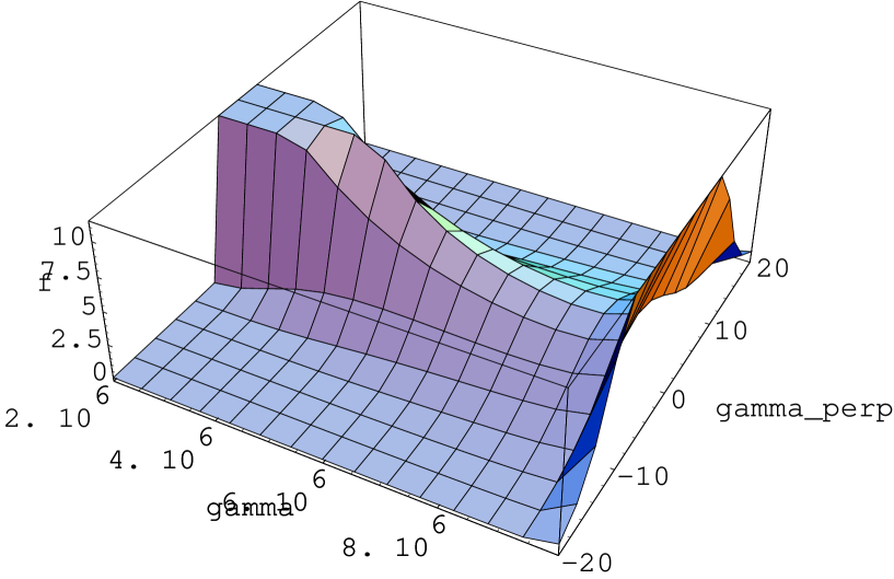
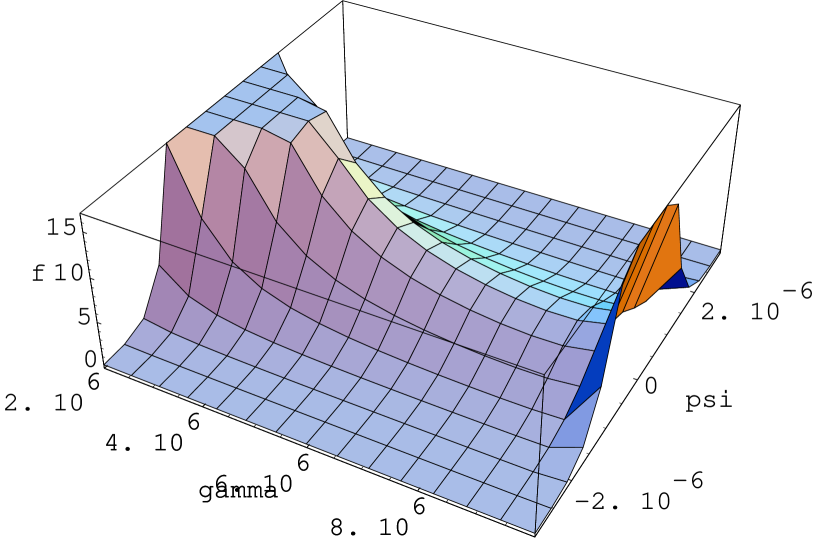
FIG. 1.: Asymptotic distribution functions in $\gamma-p_{\perp}$ and $\gamma-\psi$ spaces in arbitrary units for $\gamma_{max}=10^{7}$. The spike at the $\gamma=\gamma_{max}$ is an artifact of the initial distribution function $f(\gamma)^{0}=\delta(\gamma-\gamma_{max})$. The divergence at $\gamma=\gamma_{max}$ is weak (logarithmic) and would be removed if the more realistic nitial distribution function was used.

FIG. 2.: Asymptotic one dimensional energy density in the waves in the $\gamma$-space (arbitrary units), and the predicted observed flux in Janskys.

We can now estimate the flux per unit frequency:

$$F(\nu)=2\pi E_{k}^{2}={mc^{4}\delta^{3}\over\omega^{2}r_{e}r_{L}r_{S}^{2}}\left({\log({\gamma_{max}\omega r_{L}/(c\delta)})\over\log(\gamma_{max}/\gamma_{min})}\right)^{1/2},$$ (47)

characteristic pitch angle

$$\psi_{0}=\delta\left({\pi R_{B}r_{L}\over r_{S}^{2}}\right)^{1/2}\left({\log(\gamma_{max}/\gamma)\over\log(\gamma_{max}/\gamma_{min})}\right)^{1/4}\approx 10^{-6},$$ (48)

(which remarkably stays almost constant for a broad range of particles’ energies and also for different values of $\gamma_{min}$), and the total energy density in the waves

$$E_{tot}=\int_{\nu_{\min}}^{\nu_{\max}}F(\nu)d\nu\approx{mc^{2}\gamma_{max}\over 4\sqrt{\pi}r_{e}r_{S}^{2}\log^{1/2}(\gamma_{max}/\gamma_{min})},$$ (49)

This total energy can be compared with the kinetic energy density of the beam:

$${E_{tot}\over\gamma_{b}mc^{2}n_{GJ}}\approx\sqrt{{\pi\over\log(\gamma_{max}/\gamma_{min})}}$$ (50)

It means that some considerable fraction of the beam energy can be transformed into waves.

We can also estimate the energy flux (47) at the Earth. Assuming that distance to the pulsar is $d\approx 1$ kpc, we find

$$F^{obs}(\nu)\approx 300\,Jy\left({\nu\over 400{\rm MHz}}\right)^{-2}$$ (51)

With time, the value of $\gamma_{min}$ decreases as the particles are slowed down by the radiation reactions force. Since at the given radius, the particles with lower energies resonate with waves having larger frequencies, more energy will be transported to higher frequencies hardening the spectrum. The lower frequency cutoff is determined by the initial energy of the beam. No energy is transported to frequencies lower than

$$\omega_{min}={\omega_{B}\over\gamma_{b}\delta}$$ (52)

This simple picture, of course, will be modified due to the propagation of the flow in the inhomogeneous magnetic field of pulsar magnetosphere.

III Conclusion

In this work we investigated the new saturation mechanism for the cyclotron-Cherenkov instability of a beam in a inhomogeneous magnetic field. We showed that for the typical parameters of the pulsar magnetosphere it is possible to reach quasisteady state, in which the transverse motion of particles is determined by the balance of a radiation reaction force due to the emission at anomalous Doppler effect and the force arising in the inhomogeneous magnetic field due to the conservation of adiabatic invariant. The resulting wave intensities are sufficient to explain the observed fluxes from radio pulsars.

REFERENCES

• [1] Arons J., ApJ, 266, 215, (1983)
• [2] Kawamura K. & Suzuki I., ApJ, 217, 832, (1977)
• [3] Lominadze J.G., Machabeli G.Z. & Mikhailovsky A.B., Sov. J. Plasma Phys., 5, 748, (1979)
• [4] Machabeli G.Z. & Usov V.V, Sov. Astron. Lett., 15 , 393, (1989)
• [5] A.Z. Kazbegi, G.Z. Machabeli, G.I Melikidze, MNRAS, 253, 377 (1991)
• [6] Lyutikov M., PhD thesis, Caltech, (1998)
• [7] Lominadze J.G., Machabeli G.Z. & Usov V.V., Astroph.Space Sci., 90, 19, (1983)
• [8] Lorimer D.R. et al., MNRAS, 273, 411, (1995)
• [9] Kramer M. et al., A&A, 306, 867, (1996)
• [10] Ginzburg V.L. & Eidman V.Ya., Sov. Phys. JETPh, 36, 1300, (1959)
TABLE I.: Dimensions of the main used quantities
β€… E2​(𝐀)superscript𝐸2𝐀E^{2}({\bf k}) $E^{2}_{k}$ $n({\bf k})$ $n(k)$ $\alpha$, $\beta_{R}$ $D_{\psi\psi}$ $D_{\psi p}$ $D_{pp}$ $D$ $A$ $f(p)p^{2}dp,\,f(\gamma)d\gamma$
β€… erg ${\rm{erg\over cm^{2}}}$ 1 ${1\over cm^{2}}$ ${\rm{erg\over cm}}$ ${\rm{1\over sec}}$ ${\rm{erg\over cm}}$ ${\rm{erg^{2}\,sec\over cm^{2}}}$ ${\rm{cm^{2}\over erg\,sec}}$ ${\rm{cm}}$ 1