Muon Dynamics in a Toroidal Sector Magnet

Abstract

We present a Hamiltonian formulation of muon dynamics in toroidal sector solenoids (bent solenoid).

I INTRODUCTION

The present scenario for the cooling channel in a high brightness muon colliderref1 calls for a quasi-continuous solenoidal focusing channel. The beam line consists of a periodic array of hydrogen absorbers immersed in a solenoid with alternating focusing field and rf linacs at the zero field points.

The simple ${dE\over dx}$ energy loss in conjunction with multiple scattering and energy straggling leads to a decrease of the normalized transverse emittance. Reduction of the longitudinal emittance could be achieved by wedges of material located in dispersive regions; at least in principle, this scenario seems appropriate to obtain effective 6-D phase space reduction.ref2

A conventional chicane is a dispersion element but its use presents a serious challenge, as it is very difficult to integrate it with the solenoidal channel. The matching into the periodic solenoidal system imposes constraints on the Twiss parameters of the beam which seems not easily achievable. A possible alternative is the use of curved solenoids in conjunction with wedge absorbers as suggested by one of the authors.ref3

Solenoids and toroidal sectors have a natural place in muon collider design given the large emittance of the beam and consequently, the large transverse momentum of the initial pion beam or the decay muon beam. Bent solenoids as shown in Fig.1 were studied for use at the front end of the machine, as part of the capture channelref4 and more recently as part of a diagnostic setup to measure the position and momentum of muons.ref5

II Toroidal Sector Solenoid

If we restrict ourselves for the moment to a horizontal bending plane, the magnetic field inside of the solenoid and near the axis has a gradient (field lines are denser at smaller radius) described approximately by $\vec{B}(x,y,s)\approx B_{s}\vec{e}_{s}$ with

$$B_{s}(x,y,s)\approx{B_{s}(0,0,s)\over(1+hx)}$$ (1)

where $s$ is the coordinate along the particle trajectory and $h={1\over R_{o}}$ is the curvature at the position s, with $R_{o}$ the radius of curvature. As a consequence of the curvature of the trajectory and the corresponding magnetic gradient, the center of the particle guide orbit, averaged over the Larmor period, drifts in a direction perpendicular to the plane of bendingref6 . The combined drift velocity can be written as,

$${d\vec{r}\over dt}=v_{\|}{\vec{B}\over B}+{m_{\mu}\over 2q_{\mu}}(2v_{\|}^{2}+v_{\perp}^{2}){(\vec{R_{o}}\times\vec{B})\over(1+hx)R_{o}^{2}B^{2}}.$$ (2)

and the magnitude of the transverse drift velocity is

$$v_{\rm drift}^{T}={m_{\mu}\over 2q_{\mu}}(2v_{\|}^{2}+v_{\perp}^{2}){h\over(1+hx)B_{s}}$$ (3)

Clearly a y-position versus energy ($v_{||}$) correlation will develop as the muon beam travels along the toroidal sector solenoid.

From Eq.2 above we notice that if we include an additional vertical field, a dipole with a curvature equal to that of the bent solenoid for the reference energy, i.e.

$$\vec{B}_{D}\approx-{|B|\over v_{||}}v_{\rm drift}^{T}\vec{e}_{y}$$ (4)

then Eq.2 reduces to,

$${d\vec{r}\over dt}=v_{||}{B_{s}\over|B|}\vec{e}_{s}+(v_{||}-v_{||}^{o}){B_{D}\over|B|}\vec{e}_{y}$$ (5)

and consequently, particles with the chosen energy will not drift vertically and will remain on the axis of the bent solenoid. Those particles with larger energy will drift upward (positive y-direction) and those with lower energy downward (negative y-direction), achieving the needed dispersion. The magnitude of the dispersion is given by

$$D_{y}=2\pi{p_{o}\over q}{B_{D}\over B_{s}^{2}}=2\pi h\left({p_{o}\over qB_{s}}\right)^{2}$$ (6)

where $p_{o}$ is the chosen momentum corresponding to zero dispersion.

Figure 1: Schematic of emittance exchange system with a bent solenoid

III Dynamics in a Toroidal Solenoid. Hamiltonian Formulation

From general principles of classical mechanics and following the usual approximations in accelerator physicsref7 the normalized Hamiltonian reads,

$$H(x,p_{x},y,p_{y},z,\delta;s)\approx-{q\over p_{0}}(1+hx)A_{s}(s)-(1+\delta)hx$$

$$+{(1+hx)\over 2(1+\delta)}\left\{(p_{x}-{q\over p_{0}}A_{x})^{2}+(p_{y}-{q\over p_{0}}A_{y})^{2}\right\}$$ (7)

where the path length $s$ is the independent variable, $p_{x}\,,\,p_{y}$ are normalized momenta with respect to $p_{0}$, the initial reference total momentum $p_{0}=\sqrt{p_{x}^{2}+p_{y}^{2}+p_{s}^{2}}$; $z=s-\beta_{o}ct$, $\delta={(p-p_{0})\over p_{0}}$ and $\vec{A}=(A_{x},A_{y},A_{s})$ is the vector potential. The vector potential satisfies the gauge condition $\nabla\cdot\vec{A}=0.$

In the accelerator frame of reference, i.e. the Frenet-Serret coordinate system defined by the metric,

$$d\sigma^{2}=dx^{2}+dy^{2}+(1+hx)^{2}ds^{2}$$ (8)

the equations for the coordinate unit vectors are

$${d\vec{e_{x}}\over ds}=h(s)\vec{e_{s}}\quad,\quad{d\vec{e_{y}}\over ds}=0\quad,\quad{d\vec{e_{s}}\over ds}=-h(s)\vec{e_{x}}$$ (9)

The magnetic and electric fields are obtained from

$$\vec{B}=\nabla\times\vec{A}\qquad{\rm and}\qquad\vec{E}=c\beta_{0}{\partial\vec{A}\over\partial z}$$ (10)

with

$$\nabla\times\vec{A}= {1\over(1+hx)}\left\{\partial_{y}(1+hx)A_{s}-\partial_{s}A_{y}\right\}\vec{e}_{x}$$ (11)

$$+{1\over(1+hx)}\left\{\partial_{s}A_{x}-\partial_{x}(1+hx)A_{s}\right\}\vec{e}_{y}$$

$$+\left\{\partial_{x}A_{y}-\partial_{y}A_{x}\right\}\vec{e}_{s}$$

and

$$\nabla\cdot\vec{A}={1\over(1+hx)}\left[{\partial\over\partial x}\left(A_{x}(1+hx)\right)+{\partial\over\partial y}\left(A_{y}(1+hx)\right)+{\partial\over\partial s}A_{s}\right]$$ (12)

The lowest order approximation for a toroidal solenoidal field is given by Eq.1. The corresponding vector potential in the next order isref8 ,

$$\vec{A}=-{1\over 2}B_{o}{y\over(1+hx)}\vec{e}_{x}+{B_{o}\over 2h}\ln{(1+hx)}\vec{e}_{y}$$ (13)

and the corresponding magnetic fields are:

$$B_{x}=-{1\over(1+h(s)x)}{1\over 2h(s)}\left\{{dB_{o}\over ds}\ln{(1+h(s)x)}\right.$$

$$-\left.{B_{o}\over h(s)}h^{\prime}(s)\ln{(1+h(s)x)}+h^{\prime}(s){B_{o}x\over(1+h(s)x)}\right\}$$ (14a)

$$B_{y}=-{1\over 2(1+h(s)x)^{2}}\left\{{dB_{o}\over ds}y-h^{\prime}(s){B_{o}(s)xy\over 1+h(s)x}\right\}$$ (14b)

$$B_{s}={B_{o}\over 1+h(s)x}$$ (14c)

One possible second order approximation for the vector potential of a dipole is

$$A_{x} = -{B_{D}\over 2h(s)}{h^{\prime\prime}(s)\,x(y^{2}-{1\over 3}x^{2})\over(1+h(s)x)}$$ (15a)

$$A_{y} = {B_{D}\over 2h(s)}{h^{\prime}(s)\,xy\over(1+h(s)x)}$$ (15b)

$$A_{s} = -{B_{D}\over 2h(s)}\left\{1+h(s)\,x-h^{\prime}(s)\,(y^{2}-x^{2})\right\}$$ (15c)

Substituting the total vector potential into the Hamiltonian, and dropping some constants we can write,

$$H_{\rm tor.sol.}^{\rm dip}(x,p_{x},y,p_{y},z,\delta;s)\approx{1\over 2}(hx)^{2}-\delta hx$$

$$+{(1+hx)\over 2(1+\delta)}\left\{(p_{x}-{q\over p_{o}}A_{x})^{2}+(p_{y}-{q\over p_{o}}A_{y})^{2}\right\}$$ (16)

We have written a simple Fortran program to solve the equations of motion from the above Hamiltonian ; its result for a few representative cases of interest are shown in Fig.2.

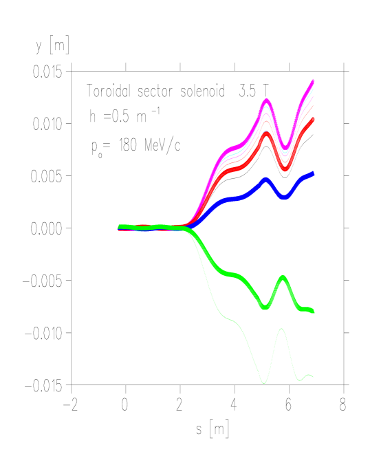
Figure 2: Example of dispersion created by a toroidal sector solenoid plus a vertical dipole. We show several tracks with energies ($\pm 1\%$) larger and smaller than the reference energy $p_{o}.$

A second order expansion of the bent solenoid magnetic field given in Eqs. 14 has been used together with a second order expansion of the dipole magnetic field in the cooling simulation program ICOOLref9 . Fig.3a shows an example of the dispersion $D_{y}$ in a bent solenoid obtained in ICOOL as a function of the dipole strength $B_{D}.$ It is apparent that the dependence of Eq. 6 on $B_{D}$ is well satisfied. Likewise, Fig 3b shows simulation results for the dispersion as a function of $B_{s}^{-2}.$ Again we see that the mentioned equation gives a good representation of the results.

Figure 3: a) Dispersion, $D_{y}$ vs. dipole magnetic field, $B_{D}$; b) Dispersion, $D_{y}$ vs. solenoid magnetic field $B_{s}^{-2}.$

IV Acknowledgements

This work was supported by the US DoE under Contract No. DE-AC02-76CH00016.

References

- (1) R. B. Palmer, presentation at FNAL Muon Collider Collaboration Meeting, July 1995, unpublished; R. B. Palmer, et al., Muon Colliders, 9th Advanced ICFA Beam Dynamics Workshop, Ed. Juan C. Gallardo, AIP Press, AIP Conference Proceedings 372, (1996).
- (2) R. B. Palmer, Cooling Theory, in preparation.
- (3) R. B. Palmer, private communication.
- (4) Collider: A Feasibility Study, New Directions for High-Energy Physics. Proceedings of the 1996 DPF/DPB Summer Study on High-Energy Physics Snowmass’96, Chapter 4; see also the Muon Collider Collaboration WEB page http://www.cap.bnl.gov/mumu/
- (5) C. Lu, K. T. McDonald and E. J. Prebys, A Detector Scenario for the Muon Cooling Experiment, Princeton//97-8, July 1997.
- (6) F. Chen, Introduction to Plasma Physics, Chap.2, Plenum Press (1979).
- (7) C. Wang and A. Chao, Notes on Lie algebraic analysis of achromats, SLAC/AP-100, Jan. 1995; E. D. Courant and H. S. Snyder, Theory of the alternating-gradient synchrotron, Ann. of Phys. 3,1 (1958); R. Ruth, Single Particle Dynamics in Circular Accelerators, Physics of Particle Accelerators, AIP Conference Proc. 153, Ed. M. Month and M. Dienes, Vol.1, pag. 150, (1987); C. Wang and A. Chao, Transfer matrices of superimposed magnets and RF cavity, SLAC/AP-106, Nov. 1996; H. Wiedemann, Particle Accelerator Physics II, pag. 51, Springer (1995).
- (8) See C. Wang and A. Chaoref7 and A. Morozov and Solov’ev, Motion of charged particles in e.m. fields, Review of Plasma Physics, vol. II, Ed. M. A. Leontovich, Consultants Bureau, Division of Plenum Publishing Company, New York (1966).
- (9) R. Fernow, ICOOL, fortran program to simulate muon ionization cooling.