Universal Statistical Behavior of Neural Spike Trains

Naama Brenner, Oded Agam, William Bialek

and Rob de Ruyter van Steveninck

NEC Research Institute, 4 Independence Way

Princeton, New Jersey 08540

 

We construct a model that predicts the statistical properties of spike trains generated by a sensory neuron. The model describes the combined effects of the neuron’s intrinsic properties, the noise in the surrounding, and the external driving stimulus. We show that the spike trains exhibit universal statistical behavior over short times, modulated by a strongly stimulus–dependent behavior over long times. These predictions are confirmed in experiments on H1, a motion–sensitive neuron in the fly visual system.

Neurons in the central nervous system communicate through the generation of stereotyped pulses, termed action potentials or spikes [1, 2]. In many cases these spikes appear to occur as a random sequence, even under conditions where external sensory stimuli are held constant. It is tempting to describe these responses in terms of stochastic models [3]. On the other hand, neurons in isolation are described quite accurately by microscopic, deterministic models of the form first proposed by Hodgkin and Huxley [4]. How do these microscopic dynamics relate to the observed statistics of spike trains? A crucial ingredient in making this link must be the properties of the noise that impinges upon the neuron, but we know relatively little about these noise sources. Here we argue that, granting certain simple assumptions, there are some universal statistical behaviors of spike trains that emerge from a wide class of models, independent of many poorly known details. These theoretical results are in good agreement with data from the fly visual system.

Many isolated neurons generate a regular sequence of action potentials when a constant current flows across the cell membrane [5, 6]. This behavior is characterized by the relation between the frequency of spikes and current, the “$f/I$ curve.” Microscopic models of neural dynamics, in the spirit of Hodgkin and Huxley, aim in part at explaining this relation between current and spike frequency [7]. Rather than trying to pass all the way from a microscopic model to a statistical description, we take the $f/I$ curve as the basic phenomenological description of the cell. We imagine that input signals $s$ determine a frequency $f(s)$ such that spikes occur when the time integral of the frequency crosses a full cycle, as indicated schematically in Fig. 1 [8].

FIG. 1.: Block diagram of the model for spike generation. The inputs are a signal $s(t)$ and a noise $n(t)$, which are added and passed through the sigmoid-like response function $f$. The modified signal then passes through an integrate-and-fire element, which generates an action potential when the integrated input exceeds a threshold (equal to one), and then resets to zero. The output of this process is a train of spikes, occuring at the instants where the threshold was crossed.

Now we would like to “embed” this model neuron in a noisy environment, such as a complex sensory network. At this step, we identify $s$ as the external signal to which the system is sensitive, generally a time dependent function $s(t)$ [9]. The noise is represented by the random function $n(t)$, added to the signal at the input of the system. The distribution of this noise defines an ensemble; averages over this ensemble will be denoted by $\langle\cdots\rangle$. For a constant input $s$, the firing rate of the neuron $r(s)$ is

$$r(s)~{}=~{}\langle f(s+n)\rangle.$$ (1)

This relates the cell’s $f/I$ curve, which characterizes the deterministic response to injected current, to the spike rate, which is the probability per unit time that the cell will spike in response to the stimulus $s$. The relation (1) is observable as the average response to repeated presentations of the same stimulus $s$. Details of the function $f(s)$ are smoothed by averaging over the noise, and hence are unobservable for a neuron in its network.

In our experiment, a live immobilized fly views various visual stimuli, chosen to excite the response of the cell H1. This large neuron is located several layers back from the eyes, and receives input from many cells. It is empirically identified as a motion detector, responding optimally to wide-field rigid horizontal motion, with strong direction selectivity [10]. The fly watches a screen with a random pattern of bars, moving horizontally with a velocity $s(t)$. We record from H1 extra-cellularly, and the response is registered as a sequence of spike timings [11]. Figure 2 shows the time-dependent firing rate $r(s(t))$ of H1 in response to a random signal $s(t)$. This signal is very slow, and so the relation (1) can be used locally in time. The plot of firing rate as a function of the instantaneous signal value (inset of Fig. 2), gives us $r(s)$, the noise-smoothed version of $f(s)$.

FIG. 2.: Firing rate of H1 as a function of time, averaged over trials: $r(t)=\langle\rho(t)\rangle_{\mbox{trials}}$ [dots], compared to the input signal $s(t)$ [solid line]. We repeat the signal many times to obtain a sampling of the noise ensemble. In the experiment, a random pattern of vertical bars is moved rigidly across the visual field with a horizontal angular velocity $s(t)$. The units of velocity are spacings of the compound eys lattice (ommatidia) per second. Inset: instantaneous relation between $r$ and $s$, which is a noise-smoothed version of the deterministic response $f(s)$ (see Eq.1).

Even for the simple model of Fig. 1, the statistical structure of spike trains can be complicated, dependent upon details in the statistics of the noise $n(t)$ and the precise form of the function $f(s)$. Universal behavior emerges, however, if we assume that the stationary noise $n(t)$ is characterized by a correlation time, $\xi_{n}$, much shorter than the typical inter-spike interval, $1/r$ [12]. With this assumption, all the formulas presented below follow from the model via straightforward calculations. We consider first the case of a constant input signal, $s(t)\!\equiv\!s$, so that the firing rate is constant, $r(s)\!\equiv\!r$.

Figure 3 shows the theoretical results together with the experimental data from the fly, for three statistical characteristics: the interval distribution (3a), the autocorrelation function (3b), and the number variance (3c). Data are presented in gray, and theory in solid black lines. All three characteristics depend on two parameters, one of which is the average firing rate $r$. It is convenient to rescale time to dimensionless units $\tau\!=\!rt$. In these units, our theory has one dimensionless parameter:

$$\gamma(s)~{}=~{}\xi_{n}\frac{\langle\delta f(s+n)^{2}\rangle}{\langle f(s+n)\rangle},$$ (2)

where $\langle\delta f(s\!+\!n)^{2}\rangle\!=\!\langle f(s\!+\!n)^{2}\rangle\!-\!\langle f(s\!+\!n)\rangle^{2}$. This parameter depends on the correlation time of the noise, $\xi_{n}$, and on the first two moments of $f(s\!+\!n)$ averaged over the noise. We will see that $\gamma$ describes the variability of the neural response, and can interpolate between a highly regular response (small $\gamma$) and a Poisson–like behavior (large $\gamma$).

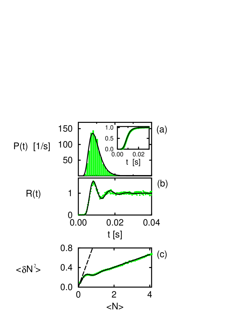
FIG. 3.: Statistical properties of spike trains in the universal regime: experiment and theory. All data are taken from an experiment in which dark and light bars forming a random pattern, move across the screen with a constant velocity of 0.12 omm/s. (a) Probability distribution of the intervals between successive spikes. Histogram of intervals from the experiment [gray bars], and Eq. 3 [line]. Inset: fraction of intervals of length less than $t$ [gray line], and integral of Eq. 3 [line]. (This way of presenting the data on intervals involves no binning.) (b) Autocorrelation function calculated from the data [gray dots], and Eq. 4 [line]. (c) Number variance as a function of number mean, as calculated from the data [gray dots], and Eq.5 [line]. For comparison, the number variance of a Poisson process, a straight line of slope 1, is shown by a dashed line.

The distribution of intervals between neighboring spikes is (Fig. 3a) [13]:

$$P(\tau)~{}~{}=~{}~{}\frac{\left(1+1/\tau\right)}{\sqrt{8\pi\gamma\tau}}~{}~{}{e}^{-\frac{(\tau-1)^{2}}{2\gamma\tau}}.$$ (3)

For very short intervals, $\tau\!\ll\!1$, the distribution decays strongly: $P(\tau)\sim e^{-1/2\gamma\tau}$; this is related to neural refractoriness, but it is not a simple absolute refractory period. For large intervals, $P(\tau)\sim e^{-\tau/2\gamma}$. The width of the distribution relative to its mean can be quantified by the coefficient of variation (the standard deviation divided by the mean [14]); for our distribution, this quantity is governed by $\gamma$, varying from zero to a constant larger than one as $\gamma$ increases. For the data presented here, $\gamma\approx 0.1$.

We can think of the spike train as a sequence of pulses at times $t_{i}$, $\rho(t)=\sum_{i}\delta(t-t_{i}).$ Then the (dimensionless) autocorrelation function of the spike train, $R(\tau)=\langle\rho(0)\rho(\tau)\rangle/\langle\rho(0)\rangle^{2}$, is (Fig. 3b):

$$R(\tau)~{}~{}=~{}~{}\sum_{k\neq 0}\frac{\left(1+k/\tau\right)}{\sqrt{8\pi\gamma\tau}}~{}~{}{e}^{-\frac{(\tau-k)^{2}}{2\gamma\tau}}~{}~{}~{}~{}~{}~{}~{}~{}~{}~{}~{}\tau>0,$$ (4)

with a symmetric expression for $\tau<0$. The correlation function is composed of an infinite sum of functions similar to the interval distribution, with shifted peaks. The number of peaks that can be resolved is proportional to $1/\gamma$: for small $\gamma$ there is a pronounced “ringing” in the correlation function, as expected for a regular spike train, while for large $\gamma$ this structure is absent, indicating an irregular or nearly Poisson sequence of spike times.

The number of spikes in a time interval of length $\tau$ is $N(\tau)=\int_{0}^{\tau}\rho(\tau^{\prime})d\tau^{\prime}$. It is a random variable and its variance can be expressed as an integral of the correlation function: $\langle\delta N^{2}\rangle=2\int_{0}^{\tau}(\tau-\tau^{\prime})R(\tau^{\prime})d\tau^{\prime}$ [2]. Using Eq. (4), we find (Fig. 3c):

$$\langle\delta N^{2}(\tau)\rangle~{}=~{}\gamma\tau+\frac{1}{2\pi^{2}}\sum_{m\neq 0}\frac{1-e^{i2\pi m\tau-2\pi^{2}m^{2}\gamma\tau}}{m^{2}(1\!+\!i\pi\gamma m)}.$$ (5)

The number variance consists of a linear term, a constant, and an infinite sum of oscillating terms. The linear term comes from the integration of the $\delta$-function part of the correlation function, at $\tau\!=\!0$ (omitted from Eq. 4). The oscillatory term decays exponentially, therefore for long times $\langle\delta N^{2}\rangle\sim\gamma\tau+c/2$, with $c=1/3+\gamma^{2}-\gamma\coth({1/\gamma})$.

Imagine now that the input signal has a time dependence, $s(t)$, and consider first the case where it is very slow. Then, the description given above holds over short time scales. Figure 4a shows the autocorrelation function of spike trains from four different experiments, with different input signals. Scaling the different data plots to dimensionless time $\tau\!=\!rt$, we see that they overlap over short times ($\tau<2$): the short–time behavior is universal. This universality cannot be explained by the existence of a constant refractory period: the plots are in dimensionless time units, and the region of universality extends well beyond any reasonable absolute refractory time. Quantitative universality requires, moreover, that the value of $\gamma$ be similar for these very different stimulus conditions. It seems likely that this approximate constancy of $\gamma$ occurs by adaptation of the fly’s visual system to the different stimulus ensembles.

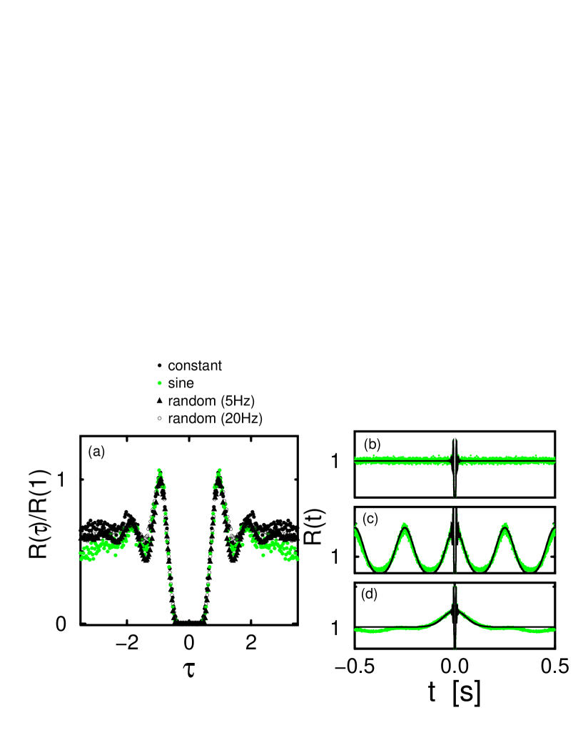
FIG. 4.: Correlation functions in the universal (a) and non-universal (b-d) regimes. (a) Data from 4 different experiments are superposed. The time axis is normalized to dimensionless units, and the horizontal axis is normalized by the value at the first peak. The graphs are very similar for short times, indicating the short–time universality, and begin to depart at longer times. (b-d) Experimental data [gray dots] are compared to theoretical results [black lines] for the different signals: constant signal (b), Sine wave signal of period 0.25 sec (c), random signal with a 5Hz bandwidth (d). Theoretical curves in (b-d) are calculated from known properties of the input signal by Eq. 6 with no adjustable parameters.

On longer times, as the oscillations of the universal regime decay, the curves begin to reflect correlations in the input signal (Fig. 4b-d). This behavior can be predicted from the model to take the approximate form [15]

$$R(\tau)~{}\approx~{}\overline{r(s(0))r(s(\tau))}~{}\sum_{k\neq 0}\frac{(1+k/\tau)}{\sqrt{8\pi\gamma\tau}}~{}e^{-\frac{(\tau-k)^{2}}{2\gamma\tau}}.~{}~{}$$ (6)

Note that the short–time behavior (in the sum) involves only the parameter $\gamma$ that can be fit in the universal regime, while the correlation function of the rates can be computed from the input/output relation in the inset of Fig. 2. In many cases simple approximation to this relation (e.g., a step function) give accurate results for the correlation function; thus we can predict correlation functions, at least approximately, with no new parameters. Figure 4 shows the long–time correlation function for various input signals: a constant signal (4b), a sine wave of period 0.25 sec (4c), and a random signal of bandwidth 5 Hz (4d). The differences between the various signals show up clearly in the long-time behavior of $R(t)$, and follow the theoretical prediction of Eq. 6 (black lines).

In conclusion, we have constructed a simple model that predicts the statistical behavior of spike trains in the neuron H1 of the fly visual system. The model is insensitive to the microscopic details of the spiking neuron; these are represented phenomenologically by the frequency-current response $f(s)$. When the model neuron is embedded in a noisy environment, the spike trains exhibit universal statistical behavior over short time scales, in which only the first two moments of $f(s)$ are important. These are represented in the theory by the two parameters $r$ and $\gamma$. In any particular case, it remains a challenge to understand the microscopic origins of these parameters, but clearly many different microscopic models can generate the same value of $\gamma$, and hence the same statistics for the spike train as measured by the inter–spike interval distribution and the short–time behavior of the autocorrelation function. On longer time scales, this universal behavior is modulated by the statistical properties of the input signal. The independence of the model on details and the weakness of the assumptions made, suggest that the results may be valid for a wider class of neurons.

REFERENCES

- [1] The Physiology of Excitable Cells, D.J. Aidley, Cambridge University Press, 1989.
- [2] Spikes: Exploring the Neural Code, F. Rieke, D. Warland, R. de Ruyter van Steveninck and W. Bialek, MIT Press 1997.
- [3] Models of the Stochastic Activity of Neurons, A.V. Holden, Lecture Notes in Biomathematics, Springer-Verlag 1976.
- [4] A.L. Hodgkin and A.F. Huxley, J. Physiol. 117, 500 (1952).
- [5] Electric Current Flow in Excitable Cells, J.J.B. Jack, D. Noble and R.W. Tsien, Clarendon Press, Oxford 1975.
- [6] D.A. McCormick, B.W. Connors, B.W. Lighthall and D.A. Prince, J. Neurophysiol. 54, 782 (1985).
- [7] T.W. Troyer and K.D. Miller, Neur. Comp. 9, 971 (1997).
- [8] One may try to derive this model as an approximation to a more microscopic description, along the lines suggested by B. Ermentrout, Neural Comp. 6, 679 (1994); 8, 979 (1996). In such an approximation, several details are expected to be added to the model: e.g. filtering of the input signals, a mechanism for the loss of memory in the integration of the frequency, noise sources intrinsic to the spiking mechanism. A more detailed discussion will be given elsewhere.
- [9] The signals used in this work were relatively slow, so that the input can be directly identified with the motion on the screen. If this motion is very fast, filtering mechanisms prior to the arrival of the signal at H1 become important, and the effective input signal should be identified as the filtered one.
- [10] Facets of Vision, Eds. D.G. Stavenga and R.C. Hardie, Springer-Verlag, 1989 [K. Hausen et al].
- [11] R. de Ruyter van Steveninck and W. Bialek, Phil. Trans. R. Soc. Lond. B (1995) 348, 321.
- [12] The spike train is mathematically defined as . Our assumption about the noise having short–range correlations implies that integrals such as are approximately Gaussian, by the central limit theorem.
- [13] The probability density of intervals is . This average gives the first passage time of the integral through the threshold, since the random variables which are being integrated are non–negative. See also G.L. Gerstein and B. Mandelbrot, Biophys. J. 4, 41 (1964); P.I.M. Johannesma, in Neural Networks - Proc. of the School on Neural Networks, Ravello 1967, Ed. E. R. Caianiello, Springer Verlag N.Y. (1968).
- [14] S. Hagiwara, Jpn. J. Physiol 4, 234 (1954).
- [15] Time may be discretized to steps of size , by which our problem becomes analogous to that of a spin chain having real values. The calculation of statistical properties is then equivalent to the calculation of expectation values over all spin configurations, with an appropriate Hamiltonian. For a constant , the Hamiltonian is that of independent spins, whereas a time–varying signal induces correlations among spins in the effective Hamiltonian. In some cases, methods of statistical mechanics (i.e. renormalization techniques) can be used to solve the problem. A universal behavior and its decoupling from a signal-dependent part appears when the noise is strong enough, and varies fast enough compared to the input signal.
- [16] Many thanks to G. Lewen, for preparing the experiments on the flies, and to N. Tishby and A. Schweitzer for helpful discussions.