Hierarchy of Fast Motions in Protein Dynamics

I Introduction

In the literature devoted to protein dynamics two classes of motions are most frequently discussed. The first comprises the slowest motions involved in the folding and various biological functions of proteins. The second class is at the opposite border of the spectrum and includes the fastest motions which limit time steps in molecular dynamics (MD) calculations and, consequently, the time scales accessible for simulation. Because of the high computer cost of long MD trajectories for biological systems, considerable efforts have always been applied to overcome these limitations. The first and most popular method is constraint MD[1, 2, 3]. Among the techniques developed in recent years one can mention, for example, multiple time scale MD[4, 5], weighted mass MD[6, 7] and internal coordinate MD (ICMD) [8, 9, 10, 11, 12]. Within the framework of this research the physical nature and the specific time scales of the fast motions in proteins have often been discussed [13]. There are several reasons, however, why this issue required the more complete analysis presented here.

One of the motivations came from recent progress in ICMD, that is dynamics simulations in the space of internal rather than Cartesian coordinates[14, 15]. By this method, proteins can be modeled as chains of rigid bodies with only torsional degrees of freedom. It is not obvious a priori what are the time step limiting motions in such models, and, in the literature, there are rather contradictory estimates of the overall prospects of ICMD compared to constraint MD [16, 17]. Another reason why this question attracts attention came from the recent results concerning the properties of the numerical algorithms commonly employed in MD, namely integrators of the Störmer-Verlet-leapfrog group[18]. It has been found that the fluctuation of the computed instantaneous total energy of a microcanonical ensemble, which is generally used as the most important test for quality of MD trajectories, is dominated by simple interpolation errors and cannot serve as a measure of accuracy. It is possible, therefore, that previous estimates of limiting step sizes were significantly biased.

Proteins have hierarchical spatial organization and this structural hierarchy is naturally mapped onto the spectrum of their motions. Namely, fast motions involve individual atoms and chemical groups while the slow ones correspond to displacements of secondary structures, domains etc. Every such movement considered separately can be characterized by a certain maximum time step, and in this sense one can say that there exists a hierarchy of fast motions and, accordingly, of step size limits. The lowest such limit is determined by bond stretching vibrations of hydrogens, but for our purposes the following few levels of this hierarchy are most interesting. Normally it is assumed that stretching of bonds between non-hydrogen atoms forms the next level[19]. However, this intuitive suggestion is not easy to verify because protein normal modes in this frequency range are not always local, and their high frequencies cannot be readily attributed to specific harmonic terms in the force field. On the other hand, normal modes with bond lengths constrained have never been studied. It should also be expected that, because of the limitations imposed by fast anharmonic motions, the hierarchy does not exactly correspond to the spectra of normal modes. All these issues are considered in detail below.

The paper is organized as a simple sequence of numerical tests on a model protein with the fastest motions suppressed one after another. Step size limits are determined by a unique test proposed and analyzed in detail elsewhere [18]. It is found that the hierarchy of step size limits is rather complicated and does not always follow common intuitive assumptions. For instance, bond stretching between non-hydrogen atoms in fact overlaps the frequency range of certain collective vibrations and, therefore, does not create a separate limitation on time steps. On the other hand, with step sizes beyond 10 fsec, anharmonic effects become dominant. In agreement with recent studies [18], leapfrog trajectories appear to hold to correct constant-energy hypersurfaces with considerably larger time steps than commonly recommended.

II Results and Discussion

Test Systems and Simulation Protocols

The main model system consists of an immunoglobulin binding domain of streptococcal protein G [20] which is a 56 residue $\alpha/\beta$ protein subunit (file 1pgb in the Protein Database [21]) with 24 bound water molecules available in the crystal structure. All hydrogens are considered explicitly giving a total of 927 atoms. In order to separate effects produced by water from those due to the protein itself similar tests were also performed for a droplet of TIP3P water molecules. The initial configuration of the droplet was obtained by taking the coordinates of the first 100 molecules closest to the center of the standard water box supplied with the AMBER package [22, 23]. Equilibration for low temperature tests was performed starting from the local energy minimum corresponding to this configuration rather than from an ice crystal structure.

In all calculations the AMBER94 force field was employed [24] without truncation of non-bonded interactions. Molecular motions were generally simulated with internal coordinates as independent variables by using Hamiltonian equations of motion and an implicit leapfrog integrator described elsewhere [15]. In one case, however, namely for normal temperature calculations with fixed bond lengths to hydrogen atoms, the standard AMBER package was employed, because the ICMD algorithm needs too many iterations for convergence with large step sizes [15]. Comparisons between ICMD trajectories and usual Cartesian MD show no essential differences [15], therefore, for consistency and convenience, internal coordinates have been preferred wherever possible.

Initial data for all numerical tests were prepared with the standard protocol described earlier [15, 18] which makes possible smooth initialization of leapfrog trajectories always from a single constant energy hypersurface. In order to simulate a virtually harmonic behavior parallel tests were performed at the very low temperature of 1K for which the equilibration protocol was modified as follows. During the first 5 psec all velocities were reassigned several times by sampling from a Maxwell distribution with T=1 K. During the following 7.5 psec velocities were rescaled periodically if the average temperature went above 2 K. This modification was necessary since in the virtually harmonic low temperature conditions energy equipartition is reached very slowly and the initial distribution over normal modes can persist for a long time. The necessary harmonic frequencies were obtained from calculated spectral densities of autocorrelation functions of appropriate generalized velocities. In all production runs the duration of the test trajectory was 10 psec.

The estimates of maximal time steps are normally made by checking conservation of the total energy of a microcanonical ensemble [25, 26]. Our approach is similar, but it accurately takes into account certain non-trivial properties of the leapfrog discretization of MD trajectories[18]. The test trajectory is repeatedly calculated always starting from the same constant-energy hypersurface. In each run certain system averages are evaluated and compared with “ideal” values, i.e. the same parameters obtained with a very small time step. The choice of such parameters must correspond to the leapfrog discretization, which means that they should be computed from on-step coordinates and half-step velocities without additional interpolations. The latter condition, together with the “smooth start”, distinguishes this approach from earlier testing strategies. These modifications are essential because they remove a significant and systematic bias present in the traditional approach which employs the time fluctuation of the instantaneous total energy as an indicator of accuracy [18].

The parameters we use are as follows: the average potential energy, $\bar{U}$, and its time variance, $D[U]$; the average kinetic energy, $\bar{K}$, computed for half-steps; the total energy, $E=\bar{U}+\bar{K}$, and its drift computed in the same way, referred to below as $E$-drift. For a sufficiently long trajectory of a Hamiltonian system $\bar{U}$, $E$ and $D[U]$ characterize the sampled hypersurface in phase space. Their deviations from the corresponding virtually ideal values characterize the bias of the sampling obtained and, therefore, can be used for accessing step size limits. The $E$-drift computed in this way is exactly zero for ideal harmonic systems [18], and is thus a good indicator of anharmonic effects.

As an example let us consider results of such testing for a completely free protein. It is seen in Fig. 1 that, below a step size of about 1.7 fsec, all the measured parameters remain approximately constant and close to the accurate values. Above this level some deviations grow rapidly. This characteristic behavior is similar to that of a simple leapfrog harmonic oscillator [18, 27]. All its properties depend upon the reduced step size $\tau=\omega h$, where $\omega$ is the frequency, and it can be shown analytically that, with small $\tau$, power series expansions for deviations of $E$ and $\bar{U}$ are dominated by the terms of the fourth and sixth orders [18]. This explains why the deviations grow rapidly beyond a certain threshold which depends mainly upon the highest frequencies in the system.

FIG. 1.: Characteristic time step dependencies obtained for a completely free protein. The corresponding low temperature plots are shown by thinner lines in (a-c). For comparison, in (a) and (c) the low temperature deviations for the total and potential energies had been scaled and shifted to fit the range of deviations observed with normal temperature. The dashed horizontal lines in (a) and (c) show the bands of acceptable deviation corresponding to variances $D[U]$ indicated by the dashed line in (d). The definition of these bands is given in the text.

In order to access the accuracy quantitatively we need to compare the deviations of average energies with some scale. An appropriate natural scale is given by the time variations of the potential energy characterized by the value of $D[U]$ shown in Fig. 1 (d). We will take a deviation of $0.1D[U]$ as the upper acceptable level for $\bar{U}$ and a two times larger value for $E$. In a harmonic system, $\bar{U}$ and $\bar{K}$ computed as described are equal [18]; so the deviation of $E$ is exactly two times that of $\bar{U}$ and it reaches its upper level simultaneously with $\bar{U}$, i.e. with the same characteristic step size denoted as $h_{c}$. The threshold levels chosen are certainly arbitrary, but they are reasonable and normally $h_{c}$ values appear similar to maximal step sizes reported in the literature. We note, however, that we will be mainly interested here in relative rather than in absolute $h_{c}$ values for different models.

Thus, the dotted line in Fig. 1 (d) marks the best estimate of the variance $D[U]$ and similar lines in Figs. 1 (a,c) show the corresponding acceptance intervals for energies. It can be seen in Figs. 1 (a) and (c) that, at normal temperature, the deviations of the total and potential energies look qualitatively different because $\bar{U}$ is affected by occasional transitions between local minima which are stochastic and cannot be properly averaged during the relatively short test trajectory. Nevertheless, both $\bar{U}$ and $E$ go beyond their acceptance intervals with $h_{c}\approx 1.7$ fsec. At low temperature, both deviations are regular, and they yield almost exactly the same $h_{c}$ value. The highest frequencies in this system are those of the bond stretching modes of hydrogens and they range from approximately 3000 cm^-1 for aliphatic groups to 3800 cm^-1 for the fastest hydroxyl groups [24, 28, 29]. It appears, therefore, that our $h_{c}$ value corresponds to $\tau\approx 1.1$ in reasonable agreement with an ideal harmonic model [18]. For a frequency of 3800 cm^-1 the stability limit of the leapfrog scheme is $h=2.78$ fsec [27], and in low temperature tests the numerical trajectory remains stable right up to this value. At normal temperature, however, a significant E-drift appears with $h>2$ fsec, which indicates that some fast anharmonic motions occur in the system, and the test trajectory could not be completed because of an explosive growth in temperature. The high E-drift can be caused, for instance, by collisions between hydrogens in non-polar contacts.

Since the data presented in Fig. 1 are redundant each case below is characterized by plots (a) and (b) alone. The deviation of the total energy is sufficient to evaluate $h_{c}$, while $\bar{U}$ always behaves similarly to plot (c). As for the value of $D[U]$ shown in Fig. 1 (d), its large and systematic deviation always results from the drift of the potential energy which is implicitly included in plot (b).

FIG. 2.: Protein models with bond length constraints: (a,b) - only bonds to hydrogen atoms fixed; (c,d) - all bond lengths fixed. The notation is similar to Figs. 1 (a) and (b).

Proteins with Constrained Bond Lengths

The two standard modes of constraining bond lengths, that is, constraining only bonds to hydrogens and constraining all bonds, yield the results shown in Fig. 2. We see that they exhibit rather similar behavior with $h_{c}$ values around 3 fsec for both low and normal temperature simulations. In proteins, the fastest bond stretching modes between non-hydrogen atoms normally occur in carboxyl groups, with frequencies around 1720 cm^-1  [29]. In our calculations, however, the fastest mode was found at 1850 cm^-1 a tryptophan side chain, which, in a harmonic case, would give a maximum step size of 5.7 fsec and $h_{c}\approx 3$. We note, therefore, that the plots in Figs. 2 (a,b) agree well with a harmonic approximation and give the expected $h_{c}$ value with only bonds to hydrogens constrained. With all bonds constrained, however, the origin of the limitation is not clear. The fastest bond angle bending modes are around 1600 cm^-1  [29], i.e. not so far, but still they should not impose limitations in this range of time steps. These limitations are evidently harmonic, however, because in low temperature tests (see Figs. 2 (a) and (c)) the two models behave almost identically. Note that they both almost reach the harmonic step size limit, with E-drift close to zero, while the $h_{c}$ values are roughly the same as those at normal temperature.

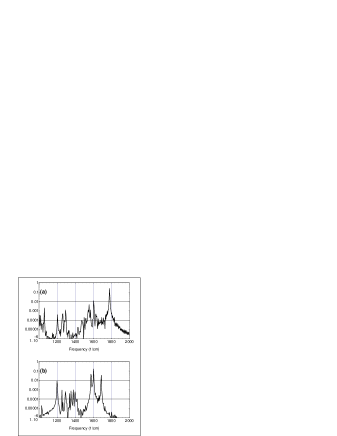
FIG. 3.: Spectral densities of velocity autocorrelation functions for H–N_ϵ–H bond angle of Lys13 for low temperature MD trajectories calculated with only bonds to hydrogen atoms fixed (a), and with all bond lengths fixed (b). The spectra had been computed from separate 40 psec runs with 1 fsec time step and all points stored. The densities are given in arbitrary scales.

An explanation to this apparently counter-intuitive behavior follows from the example shown in Fig. 3. This figure presents spectral densities of bond bending oscillations of one of the H–N_ϵ–H angles of Lys13 obtained at low temperature with the two different modes of applying bond length constraints. We see that, with fixed bonds to hydrogen atoms only, the maximum occurs at 1780 cm^-1, not very far from the fastest bond stretching. These two hydrogens are involved in hydrogen bonds with the peptide oxygen of Gly9 and a water molecule, respectively. Neither this angle, nor any of the adjacent bonds or bond angles have independent frequencies above 1700 cm^-1, nevertheless, the signal at 1780 cm^-1 is observed in the spectral densities of many valence and dihedral angles between neighboring atoms, as well as within the hydrogen bonded Gly9, indicating that this frequency corresponds to a locally distributed normal mode.

With all bond lengths fixed, this normal mode cannot remain intact, but it does not disappear, which is clear from Fig. 3 (b). Compared with Fig. 3 (a) there are many fewer signals above 1500 cm^-1, but one at 1690 cm^-1 has appeared. This peak apparently corresponds to the same fast collective mode as in Fig. 3 (a), with bond stretching eliminated, and, as we see, its frequency is just slightly reduced. Such behavior is rather characteristic of bond angle vibrations of hydrogens involved in hydrogen bonding, which explains similar step size limitations for the two modes of bond length constraint. A high frequency in this case results from a combination of several terms in the force field, rather from a single specific one, with hydrogen bonding as one of the major components. Bond length constraints affect such modes indirectly, mainly due to redistribution the system inertia. We note finally that this particular example had been selected because in both constraint modes there is only one peak above 1650 cm^-1, therefore, in the spectrum shown in Fig. 3 (a), it cannot be attributed to bond stretching. The largest independent shifts due to hydrogen bonding are observed in valence angle vibrations of hydroxyl groups and their frequencies also reach the level of 1700 cm^-1.

Water Droplet

The results of tests with a droplet of TIP3P water molecules are shown in Figs. 4 (a,b). They exhibit an $h_{c}$ value of 5 fsec, although one should note that beyond 6 fsec, with normal temperature, the E-drift grows very rapidly. It might be expected that, since in this case no purely harmonic terms are present in the force filed, the limiting motion should be anharmonic. The low temperature tests, however, yield exactly the same $h_{c}$ value and, thus, it appears that the system behaves rather similarly to the previous ones with a time step limiting frequency of approximately 1100 cm^-1. This value is close to the experimental upper boundary of the band attributed to the rotations of individual water molecules [30].

Rotation, or rather libration, of a single water molecule in a net of hydrogen bonds is certainly the fastest motion here and it can be specifically slowed down by artificially increasing the moments of inertia of the water molecule. Such water models present considerable interest for simulations where structural and thermodynamic properties are targeted, rather than kinetic ones[6]. Figures 4 (c,d) demonstrate results of such tests with an inertia ${\bf I_{ij}=\mu\delta_{ij}}$ added to oxygen atoms, where $\delta_{ij}$ is Kronecker delta and $\mu=4$ (atom mass units)$\cdot$Ų. This means that oxygens are no longer considered as point masses but as spherical rigid bodies of the same mass. With $\mu=4$ the highest frequency is expected to be reduced approximately by a factor of two, and it is seen that plots in Figs. 4 (c,d) look like those in Figs. 4 (a,b) scaled along the horizontal axis, leading to a twofold increase in $h_{c}$. Further increase of inertia gives the effect shown in Fig. 4 (e,f) where $\mu$ equals 15. Instead of an increase proportional to the square root of the added inertia we obtain $h_{c}$ around 14 fsec and 10 fsec for low and normal temperatures, respectively. In this case, therefore, we encounter a qualitatively different situation with significantly anharmonic limitations probably imposed by the translational motion of water molecules and collisions between them.

FIG. 4.: Water droplet tests. Results are shown for three different water models: (a,b) - standard TIP3P water model; (c,d) - added inertia equaled 4; (e,f) added inertia equaled 15. The notation is as in Figs. 1 (a,b).

By considering the results shown in Fig. 4 one concludes that the water model with $\mu=4$ is “well balanced” for normal temperature simulations in a sense that both its translational and rotational movements occur in the same time scale and require similar time steps. It is worth noting that the step size limits obtained here with the new test agree well with earlier results. It is known, for instance, that, with a rigid water model, all liquid structural properties are accurately reproduced up to a step size of 6 fsec [31]. A similar assertion holds for the “weighted mass” water model up to a step size of 10 fsec[6].

Proteins with Fixed Standard Amino Acid Geometry

In these calculations bond lengths and bond angles in the protein were fixed according to a standard geometry approximation [32]. The results shown in Figs. 5 (a,b) were obtained with no modifications of inertia tensors. It is seen that they strongly resemble the water droplet plots in Figs. 4 (a,b). This might mean that the step size limitations are imposed by a few water clusters around the protein, but calculations with increased water inertia yield virtually identical results. On the other hand, simultaneous weighting of water and protein hydroxyl groups yields a considerable effect as shown in Figs. 5 (c,d). The additional inertia tensor was same as in the water droplet tests above. Thus, it is evident that, in the standard geometry representation, libration of hydroxyl groups is the fastest motion, certainly due to their small inertia. The high frequency of these librations is due to hydrogen bonding rather than to the corresponding torsional potential which produces oscillations with at least three times lower frequencies.

FIG. 5.: Calculations with constraints corresponding to the standard amino acid geometry. (a,b) - with no modifications of inertia tensors; (c,d) - with inertia of water molecules and protein hydroxyl groups increased by 4; (e,f) - with inertia tensors of water molecules and protein hydroxyl and amide groups increased by 36, and masses of water oxygens equal to 72. The notation is as in Figs. 1 (a,b).

We saw above that a weighted water model with $\mu=4$ gives $h_{c}\approx 10$ fsec, and that this value already does not depend upon the dynamics of hydrogen motion. It seems that, in general, the 10 fsec level is characteristic of systems in which the time scale difference between the movements of hydrogen and non-hydrogen atoms is somehow smoothed, which is illustrated by Figs. 5 (e,f). In these calculations, in order to remove all the limitations imposed by water, the masses and inertia tensors of water oxygens were increased by 56 and 36, respectively, which gives a fourfold increase of both masses and inertia tensors compared with Figs. 4 (c,d) and, accordingly, a twofold increase in step sizes. The same inertia was added to protein hydroxyl and amide groups. In the low temperature plots in Figs. 5 (e,f), it is seen that the harmonic $h_{c}$ is shifted compared to Fig. 5 (c), which means that, in the previous model, librations of hydroxyl and amide groups produce the highest frequencies. The effect, however, takes place at low temperature only, and the characteristic time step in Fig. 5 (e) is approximately the same as in Fig. 5 (c). A similar behavior is observed in calculations with weighted inertia of other hydrogen-only rigid bodies (results not shown). The situation, therefore, appears very similar to that in the water droplet tests in Fig. 4, but in the present case fast collisions between non-hydrogen protein atoms present the limiting factor. A possible way to overcome this limitation is the RESPA approach [5] which until now has been used only within the context of Cartesian MD, but can be adapted for ICMD with the Hamiltonian equations [15] since they make possible symplectic numerical integration.

III Concluding remarks

Although the problem of time step limitations in MD simulations of biopolymers is long standing, and although the search for effective remedies has been the subject of many studies, a precise account of the effects that can create such limitations was missing in the literature. It is necessary to fill this gap in order that efforts put into the development of new methods can be effective.

The conventional view of this problem is that the step size is limited by fast harmonic motions and that these motions are produced by the stiff components of empirical potentials connected with the deformations of bonds, bond angles, planar groups etc. It has been shown here that this description takes into account only a part of step limiting factors. First, there may be many fast harmonic vibrations in which hydrogen bonding plays a major role. Second, non-bonded inter-atom interactions impose ubiquitous anharmonic limitations starting from rather small step sizes. All such factors form a complicated hierarchy which slightly differs between different empirical potentials and which is modified when constraints are imposed.

Our results suggest that the time steps currently used in MD simulations can be increased considerably with no serious loss in the accuracy of thermodynamic averages. In unconstrained calculations with AMBER potentials the estimated limit is about 1.7 fsec. Note, however, that this value is mainly connected with the frequency of OH-stretching which is high in AMBER because it close to the upper limit of experimental frequencies of free hydroxyl groups [28]. In the ENCAD potentials [33], for instance, the corresponding force constant is lowered by a factor of 2, which is why a larger step size of 2 fsec recommended by the authors is safe and could possibly even be increased further.

Constraining bonds to hydrogen atoms removes the lowest level in the hierarchy of fast motions and makes possible time steps up to 3 fsec. Constraints on other bond lengths, however, are effective only together with constraining bond angles. With fixed standard amino acid geometry, rotations of hydrogen bonded hydroxyl groups limit time steps at a 5 fsec level. The next important limitation occurs around 10 fsec and it is due to collisions between non-hydrogen protein atoms.

- [1] Ryckaert, J. P.; Ciccotti, G.; Berendsen, H. J. C. J. Comput. Phys. 1977, 23, 327.
- [2] van Gunsteren, W. F.; Berendsen, H. J. C. Mol. Phys. 1977, 34, 1311.
- [3] Ciccotti, G.; Ryckaert, J. P. Comput. Phys. Rep. 1986, 4, 345.
- [4] Pinches, M. R. S.; Tildesley, D. J.; Saville, G. Mol. Phys. 1978, 35, 639.
- [5] Tuckerman, M. E.; Berne, B. J.; Martyna, G. J. J. Chem. Phys. 1992, 97, 1990.
- [6] Pomes, R.; McCammon, J. A. Chem. Phys. Lett. 1990, 166, 425.
- [7] Mao, B.; Maggiora, G. M.; Chou, K. C. Biopolymers 1991, 31, 1077.
- [8] Pear, M. R.; Weiner, J. H. J. Chem. Phys. 1979, 71, 212.
- [9] Mazur, A. K.; Abagyan, R. A. J. Biomol. Struct. Dyn. 1989, 6, 815.
- [10] Gibson, K. D.; Scheraga, H. A. J. Comput. Chem. 1990, 11, 468.
- [11] Jain, A.; Vaidehi, N.; Rodriguez, G. J. Comput. Phys. 1993, 106, 258.
- [12] Rice, L. M.; Brünger, A. T. Proteins: Struct. Funct. Genet. 1994, 19, 277.
- [13] Brooks, C. L., III; Karplus, M.; Pettitt, B. M. Adv. Chem. Phys. 1988, 71, 175.
- [14] Mathiowetz, A. M.; Jain, A.; Karasawa, N.; Goddard, W. A., III Proteins: Struct. Funct. Genet. 1994, 20, 227.
- [15] Mazur, A. K. J. Comput. Chem. 1997, 18, 1354.
- [16] van Gunsteren, W. F.; Karplus, M. Macromolecules 1982, 15, 1528.
- [17] Dorofeyev, V. E.; Mazur, A. K. J. Comput. Phys. 1993, 107, 359.
- [18] Mazur, A. K. J. Comput. Phys. 1997, 136, 354.
- [19] van Gunsteren, W. F.; Berendsen, H. J. C. Angew. Chem. 1990, 29, 992.
- [20] Gallagher, T.; Alexander, P.; Bryan, P.; Gilliland, G. L. Biochemistry 1994, 33, 4721.
- [21] Bernstein, F. C.; Koetzle, T. F.; Williams, G. J. B.; Meyer, E. F.; Brice, M. D.; Rodgers, J. R.; Kennard, O.; Shimanouchi, T.; Tasumi, M. J. Mol. Biol 1977, 112, 535.
- [22] Pearlman, D. A.; Case, D. A.; Caldwell, J. C.; Ross, W. S.; Cheatham, T. E., III; Ferguson, D. M.; Seibel, G. L.; Singh, U. C.; Weiner, P. K.; Kollman, P. A. AMBER 4.1; University of California: San Francisco, 1995.
- [23] Jorgensen, W. L.; Chandreskhar, J.; Madura, J. D.; Impey, R. W.; Klein, M. L. J. Chem. Phys 1991, 79, 926.
- [24] Cornell, W. D.; Cieplak, P.; Bayly, C. I.; Gould, I. R.; Merz, K. M.; Ferguson, D. M.; Spellmeyer, D. C.; Fox, T.; Caldwell, J. W.; Kollman, P. A. J. Amer. Chem. Soc. 1995, 117, 5179.
- [25] Allen, M. P.; Tildesley, D. J. Computer Simulation of Liquids; Clarendon Press: Oxford, 1987.
- [26] Haile, J. M. Molecular Dynamics Simulations: Elementary Methods; Wiley-Interscience: New York, 1992.
- [27] Hockney, R. W.; Eastwood, J. W. Computer Simulation Using Particles; McGraw-Hill: New-York, 1981.
- [28] Luck, W. A. P. in Water - A Comprehensive Treatise; Franks, F., Ed.; Plenum: New York, 1972; Vol. 2, pp. 151–214.
- [29] Krimm, S.; Bandekar, J. Adv. Prot. Chem. 1986, 38, 181.
- [30] Walrafen, G. E. in Water - A Comprehensive Treatise; Franks, F., Ed.; Plenum: New York, 1972; Vol. 1, pp. 151–214.
- [31] Fincham, D. Mol. Simul. 1992, 8, 165.
- [32] Gō, N.; Scheraga, H. A. J. Chem. Phys. 1969, 51, 4751.
- [33] Levitt, M.; Hirshberg, M.; Sharon, R.; Laidig, K. E.; Daggett, V. J. Phys. Chem. 1997, 101B, 5051.